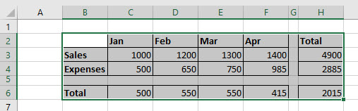
A Range is a group of selected Cells in an Excel worksheet. A Range can be rectangular or square in shape. You can select a Range by left-click, drag and release the mouse over the cells you want to select.
You can distinguish the Range in a worksheet by the hi-lighted Cells. You can see from the below image that, the color of one Cell inside the Range is not hi-lighted. This is the Active Cell of the Range. Normally, this is the first cell you clicked while selecting the Range.
For Example; you want to select the Range from Cell address D6 to G12. To select Range from D6 to G12, click and drag from Cell address D6 through Cell address G12 with mouse (or vice versa).

A Cell is identified by a Cell address. Similarly, a Range in Excel worksheet is identified by a Range Address. The syntax for forming an Excel Range address is as below.
[Cell address of Top-Left cell in the Range]:[Cell address Bottom-Right Cell in the Range]
Thus the Range address of the Range in above example is is D6:G12.
The selected Range in Excel will be removed if you click on Excel worksheet or press any arrow in keyboard.
A range is a group or block of cells in a worksheet that are selected or highlighted. Also, a range can be a group or block of cell references that are entered as an argument for a function, used to create a graph, or used to bookmark data.
The information in this article applies to Excel versions 2019, 2016, 2013, 2010, Excel Online, and Excel for Mac.
Contiguous and Non-Contiguous Ranges
A contiguous range of cells is a group of highlighted cells that are adjacent to each other, such as the range C1 to C5 shown in the image above.
A non-contiguous range consists of two or more separate blocks of cells. These blocks can be separated by rows or columns as shown by the ranges A1 to A5 and C1 to C5.
Both contiguous and non-contiguous ranges can include hundreds or even thousands of cells and span worksheets and workbooks.
Range Names
Ranges are so important in Excel and Google Spreadsheets that names can be given to specific ranges to make them easier to work with and reuse when referencing them in charts and formulas.
Select a Range in a Worksheet
When cells have been selected, they are surrounded by an outline or border. By default, this outline or border surrounds only one cell in a worksheet at a time, which is known as the active cell. Changes to a worksheet, such as data editing or formatting, affect the active cell.
When a range of more than one cell is selected, changes to the worksheet, with certain exceptions such as data entry and editing, affect all cells in the selected range.
There a number of ways to select a range in a worksheet. These include using the mouse, the keyboard, the name box, or a combination of the three.
To create a range consisting of adjacent cells, drag with the mouse or use a combination of the Shift and four arrow keys on the keyboard. To create ranges consisting of non-adjacent cells, use the mouse and keyboard or just the keyboard.
Select a Range for Use in a Formula or Chart
When entering a range of cell references as an argument for a function or when creating a chart, in addition to typing in the range manually, the range can also be selected using pointing.
Ranges are identified by the cell references or addresses of the cells in the upper left and lower right corners of the range. These two references are separated by a colon. The colon tells Excel to include all the cells between these start and endpoints.
Range vs. Array
At times the terms range and array seem to be used interchangeably for Excel and Google Sheets since both terms are related to the use of multiple cells in a workbook or file.
To be precise, the difference is because a range refers to the selection or identification of multiple cells (such as A1:A5) and an array refers to the values located in those cells (such as {1;2;5;4;3}).
Some functions, such as SUMPRODUCT and INDEX, take arrays as arguments. Other functions, such as SUMIF and COUNTIF, accept only ranges for arguments.
That’s not to say that a range of cell references cannot be entered as arguments for SUMPRODUCT and INDEX. These functions extract the values from the range and translate them into an array.
For example, the following formulas both return a result of 69 as shown in cells E1 and E2 in the image.
=SUMPRODUCT(A1:A5,C1:C5)
=SUMPRODUCT({1;2;5;4;3},{1;4;8;2;4})
On the other hand, SUMIF and COUNTIF do not accept arrays as arguments. So, while the formula below returns an answer of 3 (see cell E3 in the image), the same formula with an array would not be accepted.
COUNTIF(A1:A5,"<4")
As a result, the program displays a message box listing possible problems and corrections.
Thanks for letting us know!
Get the Latest Tech News Delivered Every Day
Subscribe
На чтение 18 мин. Просмотров 75.3k.

сэр Артур Конан Дойл
Это большая ошибка — теоретизировать, прежде чем кто-то получит данные
Эта статья охватывает все, что вам нужно знать об использовании ячеек и диапазонов в VBA. Вы можете прочитать его от начала до конца, так как он сложен в логическом порядке. Или использовать оглавление ниже, чтобы перейти к разделу по вашему выбору.
Рассматриваемые темы включают свойство смещения, чтение
значений между ячейками, чтение значений в массивы и форматирование ячеек.
Содержание
- Краткое руководство по диапазонам и клеткам
- Введение
- Важное замечание
- Свойство Range
- Свойство Cells рабочего листа
- Использование Cells и Range вместе
- Свойство Offset диапазона
- Использование диапазона CurrentRegion
- Использование Rows и Columns в качестве Ranges
- Использование Range вместо Worksheet
- Чтение значений из одной ячейки в другую
- Использование метода Range.Resize
- Чтение Value в переменные
- Как копировать и вставлять ячейки
- Чтение диапазона ячеек в массив
- Пройти через все клетки в диапазоне
- Форматирование ячеек
- Основные моменты
Краткое руководство по диапазонам и клеткам
| Функция | Принимает | Возвращает | Пример | Вид |
| Range | адреса ячеек |
диапазон ячеек |
.Range(«A1:A4») | $A$1:$A$4 |
| Cells | строка, столбец |
одна ячейка |
.Cells(1,5) | $E$1 |
| Offset | строка, столбец |
диапазон | .Range(«A1:A2») .Offset(1,2) |
$C$2:$C$3 |
| Rows | строка (-и) | одна или несколько строк |
.Rows(4) .Rows(«2:4») |
$4:$4 $2:$4 |
| Columns | столбец (-цы) |
один или несколько столбцов |
.Columns(4) .Columns(«B:D») |
$D:$D $B:$D |
Введение
Это третья статья, посвященная трем основным элементам VBA. Этими тремя элементами являются Workbooks, Worksheets и Ranges/Cells. Cells, безусловно, самая важная часть Excel. Почти все, что вы делаете в Excel, начинается и заканчивается ячейками.
Вы делаете три основных вещи с помощью ячеек:
- Читаете из ячейки.
- Пишите в ячейку.
- Изменяете формат ячейки.
В Excel есть несколько методов для доступа к ячейкам, таких как Range, Cells и Offset. Можно запутаться, так как эти функции делают похожие операции.
В этой статье я расскажу о каждом из них, объясню, почему они вам нужны, и когда вам следует их использовать.
Давайте начнем с самого простого метода доступа к ячейкам — с помощью свойства Range рабочего листа.
Важное замечание
Я недавно обновил эту статью, сейчас использую Value2.
Вам может быть интересно, в чем разница между Value, Value2 и значением по умолчанию:
' Value2
Range("A1").Value2 = 56

' Value
Range("A1").Value = 56

' По умолчанию используется значение
Range("A1") = 56
Использование Value может усечь число, если ячейка отформатирована, как валюта. Если вы не используете какое-либо свойство, по умолчанию используется Value.
Лучше использовать Value2, поскольку он всегда будет возвращать фактическое значение ячейки.
Свойство Range
Рабочий лист имеет свойство Range, которое можно использовать для доступа к ячейкам в VBA. Свойство Range принимает тот же аргумент, что и большинство функций Excel Worksheet, например: «А1», «А3: С6» и т.д.
В следующем примере показано, как поместить значение в ячейку с помощью свойства Range.
Sub ZapisVYacheiku()

    ' Запишите число в ячейку A1 на листе 1 этой книги
    ThisWorkbook.Worksheets("Лист1").Range("A1").Value2 = 67

    ' Напишите текст в ячейку A2 на листе 1 этой рабочей книги
    ThisWorkbook.Worksheets("Лист1").Range("A2").Value2 = "Иван Петров"

    ' Запишите дату в ячейку A3 на листе 1 этой книги
    ThisWorkbook.Worksheets("Лист1").Range("A3").Value2 = #11/21/2019#

End Sub
Как видно из кода, Range является членом Worksheets, которая, в свою очередь, является членом Workbook. Иерархия такая же, как и в Excel, поэтому должно быть легко понять. Чтобы сделать что-то с Range, вы должны сначала указать рабочую книгу и рабочий лист, которому она принадлежит.
В оставшейся части этой статьи я буду использовать кодовое имя для ссылки на лист.

Следующий код показывает приведенный выше пример с использованием кодового имени рабочего листа, т.е. Лист1 вместо ThisWorkbook.Worksheets («Лист1»).
Sub IspKodImya ()

    ' Запишите число в ячейку A1 на листе 1 этой книги
     Sheet1.Range("A1").Value2 = 67

    ' Напишите текст в ячейку A2 на листе 1 этой рабочей книги
    Sheet1.Range("A2").Value2 = "Иван Петров"

    ' Запишите дату в ячейку A3 на листе 1 этой книги
    Sheet1.Range("A3").Value2 = #11/21/2019#

End Sub
Вы также можете писать в несколько ячеек, используя свойство
Range
Sub ZapisNeskol()

    ' Запишите число в диапазон ячеек
    Sheet1.Range("A1:A10").Value2 = 67

    ' Написать текст в несколько диапазонов ячеек
    Sheet1.Range("B2:B5,B7:B9").Value2 = "Иван Петров"

End Sub
Свойство Cells рабочего листа
У Объекта листа есть другое свойство, называемое Cells, которое очень похоже на Range . Есть два отличия:
- Cells возвращают диапазон только одной ячейки.
- Cells принимает строку и столбец в качестве аргументов.
В приведенном ниже примере показано, как записывать значения
в ячейки, используя свойства Range и Cells.
Sub IspCells()

    ' Написать в А1
    Sheet1.Range("A1").Value2 = 10
    Sheet1.Cells(1, 1).Value2  = 10

    ' Написать в А10
    Sheet1.Range("A10").Value2 = 10
    Sheet1.Cells(10, 1).Value2  = 10

    ' Написать в E1
    Sheet1.Range("E1").Value2 = 10
    Sheet1.Cells(1, 5).Value2  = 10

End Sub
Вам должно быть интересно, когда использовать Cells, а когда Range. Использование Range полезно для доступа к одним и тем же ячейкам при каждом запуске макроса.
Например, если вы использовали макрос для вычисления суммы и
каждый раз записывали ее в ячейку A10, тогда Range подойдет для этой задачи.
Использование свойства Cells полезно, если вы обращаетесь к
ячейке по номеру, который может отличаться. Проще объяснить это на примере.
В следующем коде мы просим пользователя указать номер столбца. Использование Cells дает нам возможность использовать переменное число для столбца.
Sub ZapisVPervuyuPustuyuYacheiku()

    Dim UserCol As Integer

    ' Получить номер столбца от пользователя
    UserCol = Application.InputBox("Пожалуйста, введите номер столбца...", Type:=1)

    ' Написать текст в выбранный пользователем столбец
    Sheet1.Cells(1, UserCol).Value2 = "Иван Петров"

End Sub
В приведенном выше примере мы используем номер для столбца,
а не букву.
Чтобы использовать Range здесь, потребуется преобразовать эти значения в ссылку на
буквенно-цифровую ячейку, например, «С1». Использование свойства Cells позволяет нам
предоставить строку и номер столбца для доступа к ячейке.
Иногда вам может понадобиться вернуть более одной ячейки, используя номера строк и столбцов. В следующем разделе показано, как это сделать.
Использование Cells и Range вместе
Как вы уже видели, вы можете получить доступ только к одной ячейке, используя свойство Cells. Если вы хотите вернуть диапазон ячеек, вы можете использовать Cells с Range следующим образом:
Sub IspCellsSRange()

    With Sheet1
        ' Запишите 5 в диапазон A1: A10, используя свойство Cells
        .Range(.Cells(1, 1), .Cells(10, 1)).Value2 = 5

        ' Диапазон B1: Z1 будет выделен жирным шрифтом
        .Range(.Cells(1, 2), .Cells(1, 26)).Font.Bold = True

    End With

End Sub
Как видите, вы предоставляете начальную и конечную ячейку
диапазона. Иногда бывает сложно увидеть, с каким диапазоном вы имеете дело,
когда значением являются все числа. Range имеет свойство Address, которое
отображает буквенно-цифровую ячейку для любого диапазона. Это может
пригодиться, когда вы впервые отлаживаете или пишете код.
В следующем примере мы распечатываем адрес используемых нами
диапазонов.
Sub PokazatAdresDiapazona()

    ' Примечание. Использование подчеркивания позволяет разделить строки кода.
    With Sheet1

        ' Запишите 5 в диапазон A1: A10, используя свойство Cells
        .Range(.Cells(1, 1), .Cells(10, 1)).Value2 = 5
        Debug.Print "Первый адрес: " _
            + .Range(.Cells(1, 1), .Cells(10, 1)).Address

        ' Диапазон B1: Z1 будет выделен жирным шрифтом
        .Range(.Cells(1, 2), .Cells(1, 26)).Font.Bold = True
        Debug.Print "Второй адрес : " _
            + .Range(.Cells(1, 2), .Cells(1, 26)).Address

    End With

End Sub
В примере я использовал Debug.Print для печати в Immediate Window. Для просмотра этого окна выберите «View» -> «в Immediate Window» (Ctrl + G).


Свойство Offset диапазона
У диапазона есть свойство, которое называется Offset. Термин «Offset» относится к отсчету от исходной позиции. Он часто используется в определенных областях программирования. С помощью свойства «Offset» вы можете получить диапазон ячеек того же размера и на определенном расстоянии от текущего диапазона. Это полезно, потому что иногда вы можете выбрать диапазон на основе определенного условия. Например, на скриншоте ниже есть столбец для каждого дня недели. Учитывая номер дня (т.е. понедельник = 1, вторник = 2 и т.д.). Нам нужно записать значение в правильный столбец.

Сначала мы попытаемся сделать это без использования Offset.
' Это Sub тесты с разными значениями
Sub TestSelect()

    ' Понедельник
    SetValueSelect 1, 111.21
    ' Среда
    SetValueSelect 3, 456.99
    ' Пятница
    SetValueSelect 5, 432.25
    ' Воскресение
    SetValueSelect 7, 710.17

End Sub

' Записывает значение в столбец на основе дня
Public Sub SetValueSelect(lDay As Long, lValue As Currency)

    Select Case lDay
        Case 1: Sheet1.Range("H3").Value2 = lValue
        Case 2: Sheet1.Range("I3").Value2 = lValue
        Case 3: Sheet1.Range("J3").Value2 = lValue
        Case 4: Sheet1.Range("K3").Value2 = lValue
        Case 5: Sheet1.Range("L3").Value2 = lValue
        Case 6: Sheet1.Range("M3").Value2 = lValue
        Case 7: Sheet1.Range("N3").Value2 = lValue
    End Select

End Sub
Как видно из примера, нам нужно добавить строку для каждого возможного варианта. Это не идеальная ситуация. Использование свойства Offset обеспечивает более чистое решение.
' Это Sub тесты с разными значениями
Sub TestOffset()

    DayOffSet 1, 111.01
    DayOffSet 3, 456.99
    DayOffSet 5, 432.25
    DayOffSet 7, 710.17

End Sub

Public Sub DayOffSet(lDay As Long, lValue As Currency)

    ' Мы используем значение дня с Offset, чтобы указать правильный столбец
    Sheet1.Range("G3").Offset(, lDay).Value2 = lValue

End Sub
Как видите, это решение намного лучше. Если количество дней увеличилось, нам больше не нужно добавлять код. Чтобы Offset был полезен, должна быть какая-то связь между позициями ячеек. Если столбцы Day в приведенном выше примере были случайными, мы не могли бы использовать Offset. Мы должны были бы использовать первое решение.
Следует иметь в виду, что Offset сохраняет размер диапазона. Итак .Range («A1:A3»).Offset (1,1) возвращает диапазон B2:B4. Ниже приведены еще несколько примеров использования Offset.
Sub IspOffset()

    ' Запись в В2 - без Offset
    Sheet1.Range("B2").Offset().Value2 = "Ячейка B2"

    ' Написать в C2 - 1 столбец справа
    Sheet1.Range("B2").Offset(, 1).Value2 = "Ячейка C2"

    ' Написать в B3 - 1 строка вниз
    Sheet1.Range("B2").Offset(1).Value2 = "Ячейка B3"

    ' Запись в C3 - 1 столбец справа и 1 строка вниз
    Sheet1.Range("B2").Offset(1, 1).Value2 = "Ячейка C3"

    ' Написать в A1 - 1 столбец слева и 1 строка вверх
    Sheet1.Range("B2").Offset(-1, -1).Value2 = "Ячейка A1"

    ' Запись в диапазон E3: G13 - 1 столбец справа и 1 строка вниз
    Sheet1.Range("D2:F12").Offset(1, 1).Value2 = "Ячейки E3:G13"

End Sub
Использование диапазона CurrentRegion
CurrentRegion возвращает диапазон всех соседних ячеек в данный диапазон. На скриншоте ниже вы можете увидеть два CurrentRegion. Я добавил границы, чтобы прояснить CurrentRegion.

Строка или столбец пустых ячеек означает конец CurrentRegion.
Вы можете вручную проверить
CurrentRegion в Excel, выбрав диапазон и нажав Ctrl + Shift + *.
Если мы возьмем любой диапазон
ячеек в пределах границы и применим CurrentRegion, мы вернем диапазон ячеек во
всей области.
Например:
Range («B3»). CurrentRegion вернет диапазон B3:D14
Range («D14»). CurrentRegion вернет диапазон B3:D14
Range («C8:C9»). CurrentRegion вернет диапазон B3:D14 и так далее
Как пользоваться
Мы получаем CurrentRegion следующим образом
' CurrentRegion вернет B3:D14 из приведенного выше примера
Dim rg As Range
Set rg = Sheet1.Range("B3").CurrentRegion
Только чтение строк данных
Прочитать диапазон из второй строки, т.е. пропустить строку заголовка.
' CurrentRegion вернет B3:D14 из приведенного выше примера
Dim rg As Range
Set rg = Sheet1.Range("B3").CurrentRegion

' Начало в строке 2 - строка после заголовка
Dim i As Long
For i = 2 To rg.Rows.Count
    ' текущая строка, столбец 1 диапазона
    Debug.Print rg.Cells(i, 1).Value2
Next i
Удалить заголовок
Удалить строку заголовка (т.е. первую строку) из диапазона. Например, если диапазон — A1:D4, это возвратит A2:D4
' CurrentRegion вернет B3:D14 из приведенного выше примера
Dim rg As Range
Set rg = Sheet1.Range("B3").CurrentRegion

' Удалить заголовок
Set rg = rg.Resize(rg.Rows.Count - 1).Offset(1)

' Начните со строки 1, так как нет строки заголовка
Dim i As Long
For i = 1 To rg.Rows.Count
    ' текущая строка, столбец 1 диапазона
    Debug.Print rg.Cells(i, 1).Value2
Next i
Использование Rows и Columns в качестве Ranges
Если вы хотите что-то сделать со всей строкой или столбцом,
вы можете использовать свойство «Rows и
Columns» на рабочем листе. Они оба принимают один параметр — номер строки
или столбца, к которому вы хотите получить доступ.
Sub IspRowIColumns()

    ' Установите размер шрифта столбца B на 9
    Sheet1.Columns(2).Font.Size = 9

    ' Установите ширину столбцов от D до F
    Sheet1.Columns("D:F").ColumnWidth = 4

    ' Установите размер шрифта строки 5 до 18
    Sheet1.Rows(5).Font.Size = 18

End Sub
Использование Range вместо Worksheet
Вы также можете использовать Cella, Rows и Columns, как часть Range, а не как часть Worksheet. У вас может быть особая необходимость в этом, но в противном случае я бы избегал практики. Это делает код более сложным. Простой код — твой друг. Это уменьшает вероятность ошибок.
Код ниже выделит второй столбец диапазона полужирным. Поскольку диапазон имеет только две строки, весь столбец считается B1:B2
Sub IspColumnsVRange()

    ' Это выделит B1 и B2 жирным шрифтом.
    Sheet1.Range("A1:C2").Columns(2).Font.Bold = True

End Sub
Чтение значений из одной ячейки в другую
В большинстве примеров мы записали значения в ячейку. Мы
делаем это, помещая диапазон слева от знака равенства и значение для размещения
в ячейке справа. Для записи данных из одной ячейки в другую мы делаем то же
самое. Диапазон назначения идет слева, а диапазон источника — справа.
В следующем примере показано, как это сделать:
Sub ChitatZnacheniya()

    ' Поместите значение из B1 в A1
    Sheet1.Range("A1").Value2 = Sheet1.Range("B1").Value2

    ' Поместите значение из B3 в лист2 в ячейку A1
    Sheet1.Range("A1").Value2 = Sheet2.Range("B3").Value2

    ' Поместите значение от B1 в ячейки A1 до A5
    Sheet1.Range("A1:A5").Value2 = Sheet1.Range("B1").Value2

    ' Вам необходимо использовать свойство «Value», чтобы прочитать несколько ячеек
    Sheet1.Range("A1:A5").Value2 = Sheet1.Range("B1:B5").Value2

End Sub
Как видно из этого примера, невозможно читать из нескольких ячеек. Если вы хотите сделать это, вы можете использовать функцию копирования Range с параметром Destination.
Sub KopirovatZnacheniya()

    ' Сохранить диапазон копирования в переменной
    Dim rgCopy As Range
    Set rgCopy = Sheet1.Range("B1:B5")

    ' Используйте это для копирования из более чем одной ячейки
    rgCopy.Copy Destination:=Sheet1.Range("A1:A5")

    ' Вы можете вставить в несколько мест назначения
    rgCopy.Copy Destination:=Sheet1.Range("A1:A5,C2:C6")

End Sub
Функция Copy копирует все, включая формат ячеек. Это тот же результат, что и ручное копирование и вставка выделения. Подробнее об этом вы можете узнать в разделе «Копирование и вставка ячеек»
Использование метода Range.Resize
При копировании из одного диапазона в другой с использованием присваивания (т.е. знака равенства) диапазон назначения должен быть того же размера, что и исходный диапазон.
Использование функции Resize позволяет изменить размер
диапазона до заданного количества строк и столбцов.
Например:
Sub ResizePrimeri()

    ' Печатает А1
    Debug.Print Sheet1.Range("A1").Address

    ' Печатает A1:A2
    Debug.Print Sheet1.Range("A1").Resize(2, 1).Address

    ' Печатает A1:A5
    Debug.Print Sheet1.Range("A1").Resize(5, 1).Address

    ' Печатает A1:D1
    Debug.Print Sheet1.Range("A1").Resize(1, 4).Address

    ' Печатает A1:C3
    Debug.Print Sheet1.Range("A1").Resize(3, 3).Address

End Sub
Когда мы хотим изменить наш целевой диапазон, мы можем
просто использовать исходный размер диапазона.
Другими словами, мы используем количество строк и столбцов
исходного диапазона в качестве параметров для изменения размера:
Sub Resize()

    Dim rgSrc As Range, rgDest As Range

    ' Получить все данные в текущей области
    Set rgSrc = Sheet1.Range("A1").CurrentRegion

      ' Получить диапазон назначения
    Set rgDest = Sheet2.Range("A1")
    Set rgDest = rgDest.Resize(rgSrc.Rows.Count, rgSrc.Columns.Count)

    rgDest.Value2 = rgSrc.Value2

End Sub
Мы можем сделать изменение размера в одну строку, если нужно:
Sub Resize2()

    Dim rgSrc As Range

    ' Получить все данные в ткущей области
    Set rgSrc = Sheet1.Range("A1").CurrentRegion

    With rgSrc
        Sheet2.Range("A1").Resize(.Rows.Count, .Columns.Count) = .Value2
    End With

End Sub
Чтение Value в переменные
Мы рассмотрели, как читать из одной клетки в другую. Вы также можете читать из ячейки в переменную. Переменная используется для хранения значений во время работы макроса. Обычно вы делаете это, когда хотите манипулировать данными перед тем, как их записать. Ниже приведен простой пример использования переменной. Как видите, значение элемента справа от равенства записывается в элементе слева от равенства.
Sub IspVar()

    ' Создайте
    Dim val As Integer

    ' Читать число из ячейки
    val = Sheet1.Range("A1").Value2

    ' Добавить 1 к значению
    val = val + 1

    ' Запишите новое значение в ячейку
    Sheet1.Range("A2").Value2 = val

End Sub
Для чтения текста в переменную вы используете переменную
типа String.
Sub IspVarText()

    ' Объявите переменную типа string
    Dim sText As String

    ' Считать значение из ячейки
    sText = Sheet1.Range("A1").Value2

    ' Записать значение в ячейку
    Sheet1.Range("A2").Value2 = sText

End Sub
Вы можете записать переменную в диапазон ячеек. Вы просто
указываете диапазон слева, и значение будет записано во все ячейки диапазона.
Sub VarNeskol()

    ' Считать значение из ячейки
    Sheet1.Range("A1:B10").Value2 = 66

End Sub
Вы не можете читать из нескольких ячеек в переменную. Однако
вы можете читать массив, который представляет собой набор переменных. Мы
рассмотрим это в следующем разделе.
Как копировать и вставлять ячейки
Если вы хотите скопировать и вставить диапазон ячеек, вам не
нужно выбирать их. Это распространенная ошибка, допущенная новыми пользователями
VBA.
Вы можете просто скопировать ряд ячеек, как здесь:
Range("A1:B4").Copy Destination:=Range("C5")
При использовании этого метода копируется все — значения,
форматы, формулы и так далее. Если вы хотите скопировать отдельные элементы, вы
можете использовать свойство PasteSpecial
диапазона.
Работает так:
Range("A1:B4").Copy
Range("F3").PasteSpecial Paste:=xlPasteValues
Range("F3").PasteSpecial Paste:=xlPasteFormats
Range("F3").PasteSpecial Paste:=xlPasteFormulas
В следующей таблице приведен полный список всех типов вставок.
| Виды вставок |
| xlPasteAll |
| xlPasteAllExceptBorders |
| xlPasteAllMergingConditionalFormats |
| xlPasteAllUsingSourceTheme |
| xlPasteColumnWidths |
| xlPasteComments |
| xlPasteFormats |
| xlPasteFormulas |
| xlPasteFormulasAndNumberFormats |
| xlPasteValidation |
| xlPasteValues |
| xlPasteValuesAndNumberFormats |
Чтение диапазона ячеек в массив
Вы также можете скопировать значения, присвоив значение
одного диапазона другому.
Range("A3:Z3").Value2 = Range("A1:Z1").Value2
Значение диапазона в этом примере считается вариантом массива. Это означает, что вы можете легко читать из диапазона ячеек в массив. Вы также можете писать из массива в диапазон ячеек. Если вы не знакомы с массивами, вы можете проверить их в этой статье.
В следующем коде показан пример использования массива с
диапазоном.
Sub ChitatMassiv()

    ' Создать динамический массив
    Dim StudentMarks() As Variant

    ' Считать 26 значений в массив из первой строки
    StudentMarks = Range("A1:Z1").Value2

    ' Сделайте что-нибудь с массивом здесь

    ' Запишите 26 значений в третью строку
    Range("A3:Z3").Value2 = StudentMarks

End Sub
Имейте в виду, что массив, созданный для чтения, является
двумерным массивом. Это связано с тем, что электронная таблица хранит значения
в двух измерениях, то есть в строках и столбцах.
Пройти через все клетки в диапазоне
Иногда вам нужно просмотреть каждую ячейку, чтобы проверить значение.
Вы можете сделать это, используя цикл For Each, показанный в следующем коде.
Sub PeremeschatsyaPoYacheikam()

    ' Пройдите через каждую ячейку в диапазоне
    Dim rg As Range
    For Each rg In Sheet1.Range("A1:A10,A20")
        ' Распечатать адрес ячеек, которые являются отрицательными
        If rg.Value < 0 Then
            Debug.Print rg.Address + " Отрицательно."
        End If
    Next

End Sub
Вы также можете проходить последовательные ячейки, используя
свойство Cells и стандартный цикл For.
Стандартный цикл более гибок в отношении используемого вами
порядка, но он медленнее, чем цикл For Each.
Sub PerehodPoYacheikam()

    ' Пройдите клетки от А1 до А10
    Dim i As Long
    For i = 1 To 10
        ' Распечатать адрес ячеек, которые являются отрицательными
        If Range("A" & i).Value < 0 Then
            Debug.Print Range("A" & i).Address + " Отрицательно."
        End If
    Next

    ' Пройдите в обратном порядке, то есть от A10 до A1
    For i = 10 To 1 Step -1
        ' Распечатать адрес ячеек, которые являются отрицательными
        If Range("A" & i) < 0 Then
            Debug.Print Range("A" & i).Address + " Отрицательно."
        End If
    Next

End Sub
Форматирование ячеек
Иногда вам нужно будет отформатировать ячейки в электронной
таблице. Это на самом деле очень просто. В следующем примере показаны различные
форматы, которые можно добавить в любой диапазон ячеек.
Sub FormatirovanieYacheek()

    With Sheet1

        ' Форматировать шрифт
        .Range("A1").Font.Bold = True
        .Range("A1").Font.Underline = True
        .Range("A1").Font.Color = rgbNavy

        ' Установите числовой формат до 2 десятичных знаков
        .Range("B2").NumberFormat = "0.00"
        ' Установите числовой формат даты
        .Range("C2").NumberFormat = "dd/mm/yyyy"
        ' Установите формат чисел на общий
        .Range("C3").NumberFormat = "Общий"
        ' Установить числовой формат текста
        .Range("C4").NumberFormat = "Текст"

        ' Установите цвет заливки ячейки
        .Range("B3").Interior.Color = rgbSandyBrown

        ' Форматировать границы
        .Range("B4").Borders.LineStyle = xlDash
        .Range("B4").Borders.Color = rgbBlueViolet

    End With

End Sub
Основные моменты
Ниже приводится краткое изложение основных моментов
- Range возвращает диапазон ячеек
- Cells возвращают только одну клетку
- Вы можете читать из одной ячейки в другую
- Вы можете читать из диапазона ячеек в другой диапазон ячеек.
- Вы можете читать значения из ячеек в переменные и наоборот.
- Вы можете читать значения из диапазонов в массивы и наоборот
- Вы можете использовать цикл For Each или For, чтобы проходить через каждую ячейку в диапазоне.
- Свойства Rows и Columns позволяют вам получить доступ к диапазону ячеек этих типов
“It is a capital mistake to theorize before one has data”- Sir Arthur Conan Doyle
This post covers everything you need to know about using Cells and Ranges in VBA. You can read it from start to finish as it is laid out in a logical order. If you prefer you can use the table of contents below to go to a section of your choice.
Topics covered include Offset property, reading values between cells, reading values to arrays and formatting cells.
A Quick Guide to Ranges and Cells
| Function | Takes | Returns | Example | Gives |
|---|---|---|---|---|
|
Range |
cell address | multiple cells | .Range(«A1:A4») | $A$1:$A$4 |
| Cells | row, column | one cell | .Cells(1,5) | $E$1 |
| Offset | row, column | multiple cells | Range(«A1:A2») .Offset(1,2) |
$C$2:$C$3 |
| Rows | row(s) | one or more rows | .Rows(4) .Rows(«2:4») |
$4:$4 $2:$4 |
| Columns | column(s) | one or more columns | .Columns(4) .Columns(«B:D») |
$D:$D $B:$D |
Download the Code
The Webinar
If you are a member of the VBA Vault, then click on the image below to access the webinar and the associated source code.
(Note: Website members have access to the full webinar archive.)

Introduction
This is the third post dealing with the three main elements of VBA. These three elements are the Workbooks, Worksheets and Ranges/Cells. Cells are by far the most important part of Excel. Almost everything you do in Excel starts and ends with Cells.
Generally speaking, you do three main things with Cells
- Read from a cell.
- Write to a cell.
- Change the format of a cell.
Excel has a number of methods for accessing cells such as Range, Cells and Offset.These can cause confusion as they do similar things and can lead to confusion
In this post I will tackle each one, explain why you need it and when you should use it.
Let’s start with the simplest method of accessing cells – using the Range property of the worksheet.
Important Notes
I have recently updated this article so that is uses Value2.
You may be wondering what is the difference between Value, Value2 and the default:
' Value2
Range("A1").Value2 = 56

' Value
Range("A1").Value = 56

' Default uses value
Range("A1") = 56
Using Value may truncate number if the cell is formatted as currency. If you don’t use any property then the default is Value.
It is better to use Value2 as it will always return the actual cell value(see this article from Charle Williams.)
The Range Property
The worksheet has a Range property which you can use to access cells in VBA. The Range property takes the same argument that most Excel Worksheet functions take e.g. “A1”, “A3:C6” etc.
The following example shows you how to place a value in a cell using the Range property.
' https://excelmacromastery.com/
Public Sub WriteToCell()

    ' Write number to cell A1 in sheet1 of this workbook
    ThisWorkbook.Worksheets("Sheet1").Range("A1").Value2 = 67

    ' Write text to cell A2 in sheet1 of this workbook
    ThisWorkbook.Worksheets("Sheet1").Range("A2").Value2 = "John Smith"

    ' Write date to cell A3 in sheet1 of this workbook
    ThisWorkbook.Worksheets("Sheet1").Range("A3").Value2 = #11/21/2017#

End Sub
As you can see Range is a member of the worksheet which in turn is a member of the Workbook. This follows the same hierarchy as in Excel so should be easy to understand. To do something with Range you must first specify the workbook and worksheet it belongs to.
For the rest of this post I will use the code name to reference the worksheet.

The following code shows the above example using the code name of the worksheet i.e. Sheet1 instead of ThisWorkbook.Worksheets(“Sheet1”).
' https://excelmacromastery.com/
Public Sub UsingCodeName()

    ' Write number to cell A1 in sheet1 of this workbook
    Sheet1.Range("A1").Value2 = 67

    ' Write text to cell A2 in sheet1 of this workbook
    Sheet1.Range("A2").Value2 = "John Smith"

    ' Write date to cell A3 in sheet1 of this workbook
    Sheet1.Range("A3").Value2 = #11/21/2017#

End Sub
You can also write to multiple cells using the Range property
' https://excelmacromastery.com/
Public Sub WriteToMulti()

    ' Write number to a range of cells
    Sheet1.Range("A1:A10").Value2 = 67

    ' Write text to multiple ranges of cells
    Sheet1.Range("B2:B5,B7:B9").Value2 = "John Smith"

End Sub
You can download working examples of all the code from this post from the top of this article.
The Cells Property of the Worksheet
The worksheet object has another property called Cells which is very similar to range. There are two differences
- Cells returns a range of one cell only.
- Cells takes row and column as arguments.
The example below shows you how to write values to cells using both the Range and Cells property
' https://excelmacromastery.com/
Public Sub UsingCells()

    ' Write to A1
    Sheet1.Range("A1").Value2 = 10
    Sheet1.Cells(1, 1).Value2  = 10

    ' Write to A10
    Sheet1.Range("A10").Value2 = 10
    Sheet1.Cells(10, 1).Value2  = 10

    ' Write to E1
    Sheet1.Range("E1").Value2 = 10
    Sheet1.Cells(1, 5).Value2  = 10

End Sub
You may be wondering when you should use Cells and when you should use Range. Using Range is useful for accessing the same cells each time the Macro runs.
For example, if you were using a Macro to calculate a total and write it to cell A10 every time then Range would be suitable for this task.
Using the Cells property is useful if you are accessing a cell based on a number that may vary. It is easier to explain this with an example.
In the following code, we ask the user to specify the column number. Using Cells gives us the flexibility to use a variable number for the column.
' https://excelmacromastery.com/
Public Sub WriteToColumn()

    Dim UserCol As Integer

    ' Get the column number from the user
    UserCol = Application.InputBox(" Please enter the column...", Type:=1)

    ' Write text to user selected column
    Sheet1.Cells(1, UserCol).Value2 = "John Smith"

End Sub
In the above example, we are using a number for the column rather than a letter.
To use Range here would require us to convert these values to the letter/number cell reference e.g. “C1”. Using the Cells property allows us to provide a row and a column number to access a cell.
Sometimes you may want to return more than one cell using row and column numbers. The next section shows you how to do this.
Using Cells and Range together
As you have seen you can only access one cell using the Cells property. If you want to return a range of cells then you can use Cells with Ranges as follows
' https://excelmacromastery.com/
Public Sub UsingCellsWithRange()

    With Sheet1
        ' Write 5 to Range A1:A10 using Cells property
        .Range(.Cells(1, 1), .Cells(10, 1)).Value2 = 5

        ' Format Range B1:Z1 to be bold
        .Range(.Cells(1, 2), .Cells(1, 26)).Font.Bold = True

    End With

End Sub
As you can see, you provide the start and end cell of the Range. Sometimes it can be tricky to see which range you are dealing with when the value are all numbers. Range has a property called Address which displays the letter/ number cell reference of any range. This can come in very handy when you are debugging or writing code for the first time.
In the following example we print out the address of the ranges we are using:
' https://excelmacromastery.com/
Public Sub ShowRangeAddress()

    ' Note: Using underscore allows you to split up lines of code
    With Sheet1

        ' Write 5 to Range A1:A10 using Cells property
        .Range(.Cells(1, 1), .Cells(10, 1)).Value2 = 5
        Debug.Print "First address is : " _
            + .Range(.Cells(1, 1), .Cells(10, 1)).Address

        ' Format Range B1:Z1 to be bold
        .Range(.Cells(1, 2), .Cells(1, 26)).Font.Bold = True
        Debug.Print "Second address is : " _
            + .Range(.Cells(1, 2), .Cells(1, 26)).Address

    End With

End Sub
In the example I used Debug.Print to print to the Immediate Window. To view this window select View->Immediate Window(or Ctrl G)


You can download all the code for this post from the top of this article.
The Offset Property of Range
Range has a property called Offset. The term Offset refers to a count from the original position. It is used a lot in certain areas of programming. With the Offset property you can get a Range of cells the same size and a certain distance from the current range. The reason this is useful is that sometimes you may want to select a Range based on a certain condition. For example in the screenshot below there is a column for each day of the week. Given the day number(i.e. Monday=1, Tuesday=2 etc.) we need to write the value to the correct column.

We will first attempt to do this without using Offset.
' https://excelmacromastery.com/
' This sub tests with different values
Public Sub TestSelect()

    ' Monday
    SetValueSelect 1, 111.21
    ' Wednesday
    SetValueSelect 3, 456.99
    ' Friday
    SetValueSelect 5, 432.25
    ' Sunday
    SetValueSelect 7, 710.17

End Sub

' Writes the value to a column based on the day
Public Sub SetValueSelect(lDay As Long, lValue As Currency)

    Select Case lDay
        Case 1: Sheet1.Range("H3").Value2 = lValue
        Case 2: Sheet1.Range("I3").Value2 = lValue
        Case 3: Sheet1.Range("J3").Value2 = lValue
        Case 4: Sheet1.Range("K3").Value2 = lValue
        Case 5: Sheet1.Range("L3").Value2 = lValue
        Case 6: Sheet1.Range("M3").Value2 = lValue
        Case 7: Sheet1.Range("N3").Value2 = lValue
    End Select

End Sub
As you can see in the example, we need to add a line for each possible option. This is not an ideal situation. Using the Offset Property provides a much cleaner solution
' https://excelmacromastery.com/
' This sub tests with different values
Public Sub TestOffset()

    DayOffSet 1, 111.01
    DayOffSet 3, 456.99
    DayOffSet 5, 432.25
    DayOffSet 7, 710.17

End Sub

Public Sub DayOffSet(lDay As Long, lValue As Currency)

    ' We use the day value with offset specify the correct column
    Sheet1.Range("G3").Offset(, lDay).Value2 = lValue

End Sub
As you can see this solution is much better. If the number of days in increased then we do not need to add any more code. For Offset to be useful there needs to be some kind of relationship between the positions of the cells. If the Day columns in the above example were random then we could not use Offset. We would have to use the first solution.
One thing to keep in mind is that Offset retains the size of the range. So .Range(“A1:A3”).Offset(1,1) returns the range B2:B4. Below are some more examples of using Offset
' https://excelmacromastery.com/
Public Sub UsingOffset()

    ' Write to B2 - no offset
    Sheet1.Range("B2").Offset().Value2 = "Cell B2"

    ' Write to C2 - 1 column to the right
    Sheet1.Range("B2").Offset(, 1).Value2 = "Cell C2"

    ' Write to B3 - 1 row down
    Sheet1.Range("B2").Offset(1).Value2 = "Cell B3"

    ' Write to C3 - 1 column right and 1 row down
    Sheet1.Range("B2").Offset(1, 1).Value2 = "Cell C3"

    ' Write to A1 - 1 column left and 1 row up
    Sheet1.Range("B2").Offset(-1, -1).Value2 = "Cell A1"

    ' Write to range E3:G13 - 1 column right and 1 row down
    Sheet1.Range("D2:F12").Offset(1, 1).Value2 = "Cells E3:G13"

End Sub
Using the Range CurrentRegion
CurrentRegion returns a range of all the adjacent cells to the given range.
In the screenshot below you can see the two current regions. I have added borders to make the current regions clear.

A row or column of blank cells signifies the end of a current region.
You can manually check the CurrentRegion in Excel by selecting a range and pressing Ctrl + Shift + *.
If we take any range of cells within the border and apply CurrentRegion, we will get back the range of cells in the entire area.
For example
Range(“B3”).CurrentRegion will return the range B3:D14
Range(“D14”).CurrentRegion will return the range B3:D14
Range(“C8:C9”).CurrentRegion will return the range B3:D14
and so on
How to Use
We get the CurrentRegion as follows
' Current region will return B3:D14 from above example
Dim rg As Range
Set rg = Sheet1.Range("B3").CurrentRegion
Read Data Rows Only
Read through the range from the second row i.e.skipping the header row
' Current region will return B3:D14 from above example
Dim rg As Range
Set rg = Sheet1.Range("B3").CurrentRegion

' Start at row 2 - row after header
Dim i As Long
For i = 2 To rg.Rows.Count
    ' current row, column 1 of range
    Debug.Print rg.Cells(i, 1).Value2
Next i
Remove Header
Remove header row(i.e. first row) from the range. For example if range is A1:D4 this will return A2:D4
' Current region will return B3:D14 from above example
Dim rg As Range
Set rg = Sheet1.Range("B3").CurrentRegion

' Remove Header
Set rg = rg.Resize(rg.Rows.Count - 1).Offset(1)

' Start at row 1 as no header row
Dim i As Long
For i = 1 To rg.Rows.Count
    ' current row, column 1 of range
    Debug.Print rg.Cells(i, 1).Value2
Next i
Using Rows and Columns as Ranges
If you want to do something with an entire Row or Column you can use the Rows or Columns property of the Worksheet. They both take one parameter which is the row or column number you wish to access
' https://excelmacromastery.com/
Public Sub UseRowAndColumns()

    ' Set the font size of column B to 9
    Sheet1.Columns(2).Font.Size = 9

    ' Set the width of columns D to F
    Sheet1.Columns("D:F").ColumnWidth = 4

    ' Set the font size of row 5 to 18
    Sheet1.Rows(5).Font.Size = 18

End Sub
Using Range in place of Worksheet
You can also use Cells, Rows and Columns as part of a Range rather than part of a Worksheet. You may have a specific need to do this but otherwise I would avoid the practice. It makes the code more complex. Simple code is your friend. It reduces the possibility of errors.
The code below will set the second column of the range to bold. As the range has only two rows the entire column is considered B1:B2
' https://excelmacromastery.com/
Public Sub UseColumnsInRange()

    ' This will set B1 and B2 to be bold
    Sheet1.Range("A1:C2").Columns(2).Font.Bold = True

End Sub
You can download all the code for this post from the top of this article.
Reading Values from one Cell to another
In most of the examples so far we have written values to a cell. We do this by placing the range on the left of the equals sign and the value to place in the cell on the right. To write data from one cell to another we do the same. The destination range goes on the left and the source range goes on the right.
The following example shows you how to do this:
' https://excelmacromastery.com/
Public Sub ReadValues()

    ' Place value from B1 in A1
    Sheet1.Range("A1").Value2 = Sheet1.Range("B1").Value2

    ' Place value from B3 in sheet2 to cell A1
    Sheet1.Range("A1").Value2 = Sheet2.Range("B3").Value2

    ' Place value from B1 in cells A1 to A5
    Sheet1.Range("A1:A5").Value2 = Sheet1.Range("B1").Value2

    ' You need to use the "Value" property to read multiple cells
    Sheet1.Range("A1:A5").Value2 = Sheet1.Range("B1:B5").Value2

End Sub
As you can see from this example it is not possible to read from multiple cells. If you want to do this you can use the Copy function of Range with the Destination parameter
' https://excelmacromastery.com/
Public Sub CopyValues()

    ' Store the copy range in a variable
    Dim rgCopy As Range
    Set rgCopy = Sheet1.Range("B1:B5")

    ' Use this to copy from more than one cell
    rgCopy.Copy Destination:=Sheet1.Range("A1:A5")

    ' You can paste to multiple destinations
    rgCopy.Copy Destination:=Sheet1.Range("A1:A5,C2:C6")

End Sub
The Copy function copies everything including the format of the cells. It is the same result as manually copying and pasting a selection. You can see more about it in the Copying and Pasting Cells section.
Using the Range.Resize Method
When copying from one range to another using assignment(i.e. the equals sign), the destination range must be the same size as the source range.
Using the Resize function allows us to resize a range to a given number of rows and columns.
For example:
' https://excelmacromastery.com/
Sub ResizeExamples()

    ' Prints A1
    Debug.Print Sheet1.Range("A1").Address

    ' Prints A1:A2
    Debug.Print Sheet1.Range("A1").Resize(2, 1).Address

    ' Prints A1:A5
    Debug.Print Sheet1.Range("A1").Resize(5, 1).Address

    ' Prints A1:D1
    Debug.Print Sheet1.Range("A1").Resize(1, 4).Address

    ' Prints A1:C3
    Debug.Print Sheet1.Range("A1").Resize(3, 3).Address

End Sub
When we want to resize our destination range we can simply use the source range size.
In other words, we use the row and column count of the source range as the parameters for resizing:
' https://excelmacromastery.com/
Sub Resize()

    Dim rgSrc As Range, rgDest As Range

    ' Get all the data in the current region
    Set rgSrc = Sheet1.Range("A1").CurrentRegion

      ' Get the range destination
    Set rgDest = Sheet2.Range("A1")
    Set rgDest = rgDest.Resize(rgSrc.Rows.Count, rgSrc.Columns.Count)

    rgDest.Value2 = rgSrc.Value2

End Sub
We can do the resize in one line if we prefer:
' https://excelmacromastery.com/
Sub ResizeOneLine()

    Dim rgSrc As Range

    ' Get all the data in the current region
    Set rgSrc = Sheet1.Range("A1").CurrentRegion

    With rgSrc
        Sheet2.Range("A1").Resize(.Rows.Count, .Columns.Count).Value2 = .Value2
    End With

End Sub
Reading Values to variables
We looked at how to read from one cell to another. You can also read from a cell to a variable. A variable is used to store values while a Macro is running. You normally do this when you want to manipulate the data before writing it somewhere. The following is a simple example using a variable. As you can see the value of the item to the right of the equals is written to the item to the left of the equals.
' https://excelmacromastery.com/
Public Sub UseVariables()

    ' Create
    Dim number As Long

    ' Read number from cell
    number = Sheet1.Range("A1").Value2

    ' Add 1 to value
    number = number + 1

    ' Write new value to cell
    Sheet1.Range("A2").Value2 = number

End Sub
To read text to a variable you use a variable of type String:
' https://excelmacromastery.com/
Public Sub UseVariableText()

    ' Declare a variable of type string
    Dim text As String

    ' Read value from cell
    text = Sheet1.Range("A1").Value2

    ' Write value to cell
    Sheet1.Range("A2").Value2 = text

End Sub
You can write a variable to a range of cells. You just specify the range on the left and the value will be written to all cells in the range.
' https://excelmacromastery.com/
Public Sub VarToMulti()

    ' Read value from cell
    Sheet1.Range("A1:B10").Value2 = 66

End Sub
You cannot read from multiple cells to a variable. However you can read to an array which is a collection of variables. We will look at doing this in the next section.
How to Copy and Paste Cells
If you want to copy and paste a range of cells then you do not need to select them. This is a common error made by new VBA users.
Note: We normally use Range.Copy when we want to copy formats, formulas, validation. If we want to copy values it is not the most efficient method.
I have written a complete guide to copying data in Excel VBA here.
You can simply copy a range of cells like this:
Range("A1:B4").Copy Destination:=Range("C5")
Using this method copies everything – values, formats, formulas and so on. If you want to copy individual items you can use the PasteSpecial property of range.
It works like this
Range("A1:B4").Copy
Range("F3").PasteSpecial Paste:=xlPasteValues
Range("F3").PasteSpecial Paste:=xlPasteFormats
Range("F3").PasteSpecial Paste:=xlPasteFormulas
The following table shows a full list of all the paste types
| Paste Type |
|---|
| xlPasteAll |
| xlPasteAllExceptBorders |
| xlPasteAllMergingConditionalFormats |
| xlPasteAllUsingSourceTheme |
| xlPasteColumnWidths |
| xlPasteComments |
| xlPasteFormats |
| xlPasteFormulas |
| xlPasteFormulasAndNumberFormats |
| xlPasteValidation |
| xlPasteValues |
| xlPasteValuesAndNumberFormats |
Reading a Range of Cells to an Array
You can also copy values by assigning the value of one range to another.
Range("A3:Z3").Value2 = Range("A1:Z1").Value2
The value of range in this example is considered to be a variant array. What this means is that you can easily read from a range of cells to an array. You can also write from an array to a range of cells. If you are not familiar with arrays you can check them out in this post.
The following code shows an example of using an array with a range:
' https://excelmacromastery.com/
Public Sub ReadToArray()

    ' Create dynamic array
    Dim StudentMarks() As Variant

    ' Read 26 values into array from the first row
    StudentMarks = Range("A1:Z1").Value2

    ' Do something with array here

    ' Write the 26 values to the third row
    Range("A3:Z3").Value2 = StudentMarks

End Sub
Keep in mind that the array created by the read is a 2 dimensional array. This is because a spreadsheet stores values in two dimensions i.e. rows and columns
Going through all the cells in a Range
Sometimes you may want to go through each cell one at a time to check value.
You can do this using a For Each loop shown in the following code
' https://excelmacromastery.com/
Public Sub TraversingCells()

    ' Go through each cells in the range
    Dim rg As Range
    For Each rg In Sheet1.Range("A1:A10,A20")
        ' Print address of cells that are negative
        If rg.Value < 0 Then
            Debug.Print rg.Address + " is negative."
        End If
    Next

End Sub
You can also go through consecutive Cells using the Cells property and a standard For loop.
The standard loop is more flexible about the order you use but it is slower than a For Each loop.
' https://excelmacromastery.com/
Public Sub TraverseCells()

    ' Go through cells from A1 to A10
    Dim i As Long
    For i = 1 To 10
        ' Print address of cells that are negative
        If Range("A" & i).Value < 0 Then
            Debug.Print Range("A" & i).Address + " is negative."
        End If
    Next

    ' Go through cells in reverse i.e. from A10 to A1
    For i = 10 To 1 Step -1
        ' Print address of cells that are negative
        If Range("A" & i) < 0 Then
            Debug.Print Range("A" & i).Address + " is negative."
        End If
    Next

End Sub
Formatting Cells
Sometimes you will need to format the cells the in spreadsheet. This is actually very straightforward. The following example shows you various formatting you can add to any range of cells
' https://excelmacromastery.com/
Public Sub FormattingCells()

    With Sheet1

        ' Format the font
        .Range("A1").Font.Bold = True
        .Range("A1").Font.Underline = True
        .Range("A1").Font.Color = rgbNavy

        ' Set the number format to 2 decimal places
        .Range("B2").NumberFormat = "0.00"
        ' Set the number format to a date
        .Range("C2").NumberFormat = "dd/mm/yyyy"
        ' Set the number format to general
        .Range("C3").NumberFormat = "General"
        ' Set the number format to text
        .Range("C4").NumberFormat = "Text"

        ' Set the fill color of the cell
        .Range("B3").Interior.Color = rgbSandyBrown

        ' Format the borders
        .Range("B4").Borders.LineStyle = xlDash
        .Range("B4").Borders.Color = rgbBlueViolet

    End With

End Sub
Main Points
The following is a summary of the main points
- Range returns a range of cells
- Cells returns one cells only
- You can read from one cell to another
- You can read from a range of cells to another range of cells.
- You can read values from cells to variables and vice versa.
- You can read values from ranges to arrays and vice versa
- You can use a For Each or For loop to run through every cell in a range.
- The properties Rows and Columns allow you to access a range of cells of these types
What’s Next?
Free VBA Tutorial If you are new to VBA or you want to sharpen your existing VBA skills then why not try out the The Ultimate VBA Tutorial.
Related Training: Get full access to the Excel VBA training webinars and all the tutorials.
(NOTE: Planning to build or manage a VBA Application? Learn how to build 10 Excel VBA applications from scratch.)
Find Range in Excel (Table of Contents)
- Range in Excel
- How to Find Range in Excel?
Range in Excel
Whenever we talk about the range in excel, it can be one cell or can be a collection of cells. It can be the adjacent cells or non-adjacent cells in the dataset.
What is Range in Excel & its Formula?
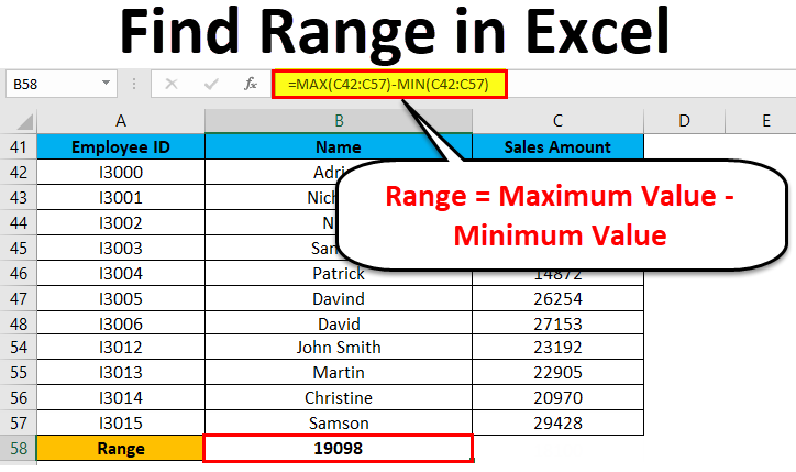
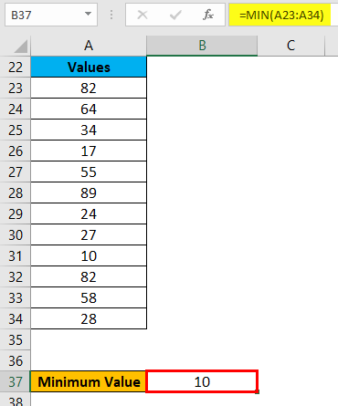
A range is the collection of values spread between the Maximum value and the Minimum value. A range is a difference between the Largest (maximum) value and the Shortest (minimum) value in a given dataset in mathematical terms.
Range defines the spread of values in any dataset. It calculates by a simple formula like below:
Range = Maximum Value – Minimum Value
How to Find Range in Excel?
Finding a range is a very simple process, and it is calculated using the Excel in-built functions MAX and MIN. Let’s understand the working of finding a range in excel with some examples.
You can download this Find Range Excel Template here – Find Range Excel Template
Range in Excel – Example #1
We have given below a list of values:
23, 11, 45, 21, 2, 60, 10, 35
The largest number in the above-given range is 60, and the smallest number is 2.
Thus, the Range = 60-2 = 58
Explanation:
- In this above example, the Range is 58 in the given dataset, which defines the span of the dataset. It gave you a visual indication of the range as we are looking for the highest and smallest point.
- If the dataset is large, it gives you the widespread of the result.
- If the dataset is small, it gives you a closely centered result.
A process of defining the range in Excel
For defining the range, we need to find out the maximum and minimum values of the dataset. In this process, two function plays a very important role. They are:
- MAX
- MIN
Use of MAX function:
Let’s take an example to understand the usage of this function.
Range in Excel – Example #2
We have given some set of values:
For finding the maximum value from the dataset, we will apply here the MAX function as below screenshot:
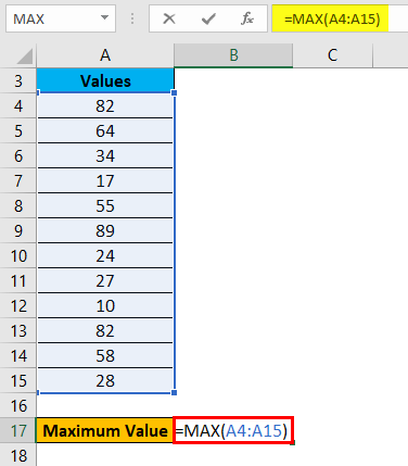
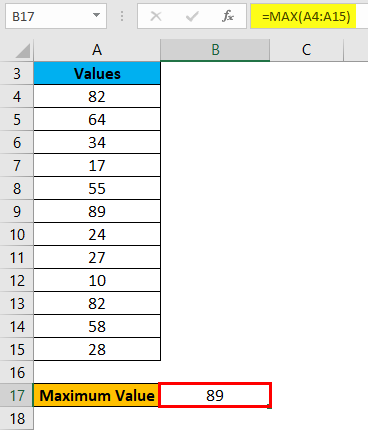
Hit enter, and it will give you the maximum value. The result is shown below:
Range in Excel – Example #3
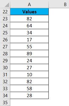
Use of MIN function:
Let’s take the same above dataset to understand the usage of this function.
For calculating the minimum value from the given dataset, we will apply the MIN function here as per the below screenshot.
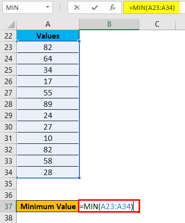
Press ENTER key, and it will give you the minimum value. The result is given below:
Now you can find out the range of the dataset after taking the difference between Maximum and Minimum value.
We can reduce the steps for calculating the range of a dataset by using the MAX and MIN functions together in one line.
For this, we again take an example to understand the process.
Range in Excel – Example #4
Let’s assume the below dataset of a company employee with their achieved sales target.
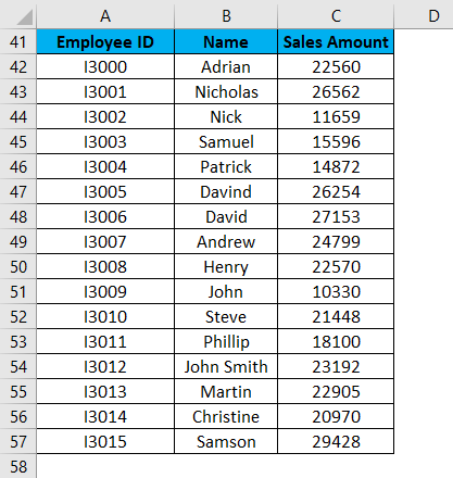
Now for identifying the span of sales amount in the above dataset, we will calculate the range. For this, we will follow the same procedure as we did in the above examples.
We will apply the MAX and MIN functions for calculating the Maximum and Minimum sales amount in the data.
For finding the range of sales amount, we will apply the below formula:
Range = Maximum Value – Minimum Value
Refer to the below screenshot:
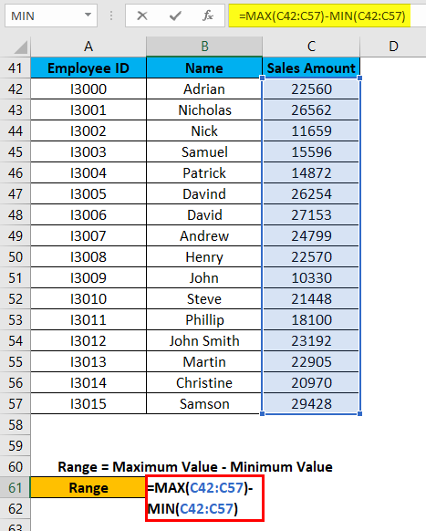
Press Enter key, and it will give you the range of the dataset. The result is shown below:
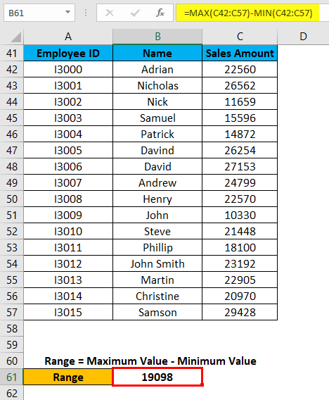
As we can see in the above screenshot, we applied the MAX and MIN formulas in one line, and by calculating their results difference, we found the range of the dataset.
Things to Remember
- If the values are available in the non-adjacent cells, you want to find out the range; you can pass the cell address individually, separated with a comma as an argument of the MAX and MIN functions.
- We can reduce the steps for calculating the range by applying MAX and MIN functions in one line. (Refer to Example 4 for your reference)
Recommended Articles
This has been a guide to Range in Excel. Here we discuss how to find Range in Excel along with excel examples and downloadable excel template. You may learn more about Excel from the following articles –
- Excel Function for Range
- Excel Named Range
- VBA Range
- VBA Selecting Range
Термин Объекты Excel (понимаемый в широком смысле, как объектная модель Excel) включает в себя элементы, из которых состоит любая рабочая книга Excel. Это, например, рабочие листы (Worksheets), строки (Rows), столбцы (Columns), диапазоны ячеек (Ranges) и сама рабочая книга Excel (Workbook) в том числе. Каждый объект Excel имеет набор свойств, которые являются его неотъемлемой частью.
Например, объект Worksheet (рабочий лист) имеет свойства Name (имя), Protection (защита), Visible (видимость), Scroll Area (область прокрутки) и так далее. Таким образом, если в процессе выполнения макроса требуется скрыть рабочий лист, то достаточно изменить свойство Visible этого листа.
В Excel VBA существует особый тип объектов – коллекция. Как можно догадаться из названия, коллекция ссылается на группу (или коллекцию) объектов Excel. Например, коллекция Rows – это объект, содержащий все строки рабочего листа.
Доступ ко всем основным объектам Excel может быть осуществлён (прямо или косвенно) через объект Workbooks, который является коллекцией всех открытых в данный момент рабочих книг. Каждая рабочая книга содержит объект Sheets – коллекция, которая включает в себя все рабочие листы и листы с диаграммами рабочей книги. Каждый объект Worksheet состоит из коллекции Rows – в неё входят все строки рабочего листа, и коллекции Columns – все столбцы рабочего листа, и так далее.
В следующей таблице перечислены некоторые наиболее часто используемые объекты Excel. Полный перечень объектов Excel VBA можно найти на сайте Microsoft Office Developer (на английском).
| Объект | Описание |
|---|---|
| Application | Приложение Excel. |
| Workbooks | Коллекция всех открытых в данный момент рабочих книг в текущем приложении Excel. Доступ к какой-то конкретной рабочей книге может быть осуществлён через объект Workbooks при помощи числового индекса рабочей книги или её имени, например, Workbooks(1) или Workbooks(«Книга1»). |
| Workbook | Объект Workbook – это рабочая книга. Доступ к ней может быть выполнен через коллекцию Workbooks при помощи числового индекса или имени рабочей книги (см. выше). Для доступа к активной в данный момент рабочей книге можно использовать ActiveWorkbook.
Из объекта Workbook можно получить доступ к объекту Sheets, который является коллекцией всех листов рабочей книги (рабочие листы и диаграммы), а также к объекту Worksheets, который представляет из себя коллекцию всех рабочих листов книги Excel. |
| Sheets | Объект Sheets– это коллекция всех листов рабочей книги. Это могут быть как рабочие листы, так и диаграммы на отдельном листе. Доступ к отдельному листу из коллекции Sheets можно получить при помощи числового индекса листа или его имени, например, Sheets(1) или Sheets(«Лист1»). |
| Worksheets | Объект Worksheets – это коллекция всех рабочих листов в рабочей книге (то есть, все листы, кроме диаграмм на отдельном листе). Доступ к отдельному рабочему листу из коллекции Worksheets можно получить при помощи числового индекса рабочего листа или его имени, например, Worksheets(1) или Worksheets(«Лист1»). |
| Worksheet | Объект Worksheet – это отдельный рабочий лист книги Excel. Доступ к нему можно получить при помощи числового индекса рабочего листа или его имени (см. выше).
Кроме этого Вы можете использовать ActiveSheet для доступа к активному в данный момент рабочему листу. Из объекта Worksheet можно получить доступ к объектам Rows и Columns, которые являются коллекцией объектов Range, ссылающихся на строки и столбцы рабочего листа. А также можно получить доступ к отдельной ячейке или к любому диапазону смежных ячеек на рабочем листе. |
| Rows | Объект Rows – это коллекция всех строк рабочего листа. Объект Range, состоящий из отдельной строки рабочего листа, может быть доступен по номеру этой строки, например, Rows(1). |
| Columns | Объект Columns – это коллекция всех столбцов рабочего листа. Объект Range, состоящий из отдельного столбца рабочего листа, может быть доступен по номеру этого столбца, например, Columns(1). |
| Range | Объект Range – это любое количество смежных ячеек на рабочем листе. Это может быть одна ячейка или все ячейки листа.
Доступ к диапазону, состоящему из единственной ячейки, может быть осуществлён через объект Worksheet при помощи свойства Cells, например, Worksheet.Cells(1,1). По-другому ссылку на диапазон можно записать, указав адреса начальной и конечной ячеек. Их можно записать через двоеточие или через запятую. Например, Worksheet.Range(«A1:B10») или Worksheet.Range(«A1», «B10») или Worksheet.Range(Cells(1,1), Cells(10,2)). Обратите внимание, если в адресе Range вторая ячейка не указана (например, Worksheet.Range(«A1») или Worksheet.Range(Cells(1,1)), то будет выбран диапазон, состоящий из единственной ячейки. |
Приведённая выше таблица показывает, как выполняется доступ к объектам Excel через родительские объекты. Например, ссылку на диапазон ячеек можно записать вот так:
Workbooks("Книга1").Worksheets("Лист1").Range("A1:B10")
Содержание
- Присваивание объекта переменной
- Активный объект
- Смена активного объекта
- Свойства объектов
- Методы объектов
- Рассмотрим несколько примеров
- Пример 1
- Пример 2
- Пример 3
Присваивание объекта переменной
В Excel VBA объект может быть присвоен переменной при помощи ключевого слова Set:
Dim DataWb As Workbook
Set DataWb = Workbooks("Книга1.xlsx")
Активный объект
В любой момент времени в Excel есть активный объект Workbook – это рабочая книга, открытая в этот момент. Точно так же существует активный объект Worksheet, активный объект Range и так далее.
Сослаться на активный объект Workbook или Sheet в коде VBA можно как на ActiveWorkbook или ActiveSheet, а на активный объект Range – как на Selection.
Если в коде VBA записана ссылка на рабочий лист, без указания к какой именно рабочей книге он относится, то Excel по умолчанию обращается к активной рабочей книге. Точно так же, если сослаться на диапазон, не указывая определённую рабочую книгу или лист, то Excel по умолчанию обратится к активному рабочему листу в активной рабочей книге.
Таким образом, чтобы сослаться на диапазон A1:B10 на активном рабочем листе активной книги, можно записать просто:
Смена активного объекта
Если в процессе выполнения программы требуется сделать активной другую рабочую книгу, другой рабочий лист, диапазон и так далее, то для этого нужно использовать методы Activate или Select вот таким образом:
Sub ActivateAndSelect()

   Workbooks("Книга2").Activate
   Worksheets("Лист2").Select
   Worksheets("Лист2").Range("A1:B10").Select
   Worksheets("Лист2").Range("A5").Activate

End Sub
Методы объектов, в том числе использованные только что методы Activate или Select, далее будут рассмотрены более подробно.
Свойства объектов
Каждый объект VBA имеет заданные для него свойства. Например, объект Workbook имеет свойства Name (имя), RevisionNumber (количество сохранений), Sheets (листы) и множество других. Чтобы получить доступ к свойствам объекта, нужно записать имя объекта, затем точку и далее имя свойства. Например, имя активной рабочей книги может быть доступно вот так: ActiveWorkbook.Name. Таким образом, чтобы присвоить переменной wbName имя активной рабочей книги, можно использовать вот такой код:
Dim wbName As String
wbName = ActiveWorkbook.Name
Ранее мы показали, как объект Workbook может быть использован для доступа к объекту Worksheet при помощи такой команды:
Workbooks("Книга1").Worksheets("Лист1")
Это возможно потому, что коллекция Worksheets является свойством объекта Workbook.
Некоторые свойства объекта доступны только для чтения, то есть их значения пользователь изменять не может. В то же время существуют свойства, которым можно присваивать различные значения. Например, чтобы изменить название активного листа на «Мой рабочий лист«, достаточно присвоить это имя свойству Name активного листа, вот так:
ActiveSheet.Name = "Мой рабочий лист"
Методы объектов
Объекты VBA имеют методы для выполнения определённых действий. Методы объекта – это процедуры, привязанные к объектам определённого типа. Например, объект Workbook имеет методы Activate, Close, Save и ещё множество других.
Для того, чтобы вызвать метод объекта, нужно записать имя объекта, точку и имя метода. Например, чтобы сохранить активную рабочую книгу, можно использовать вот такую строку кода:
Как и другие процедуры, методы могут иметь аргументы, которые передаются методу при его вызове. Например, метод Close объекта Workbook имеет три необязательных аргумента, которые определяют, должна ли быть сохранена рабочая книга перед закрытием и тому подобное.
Чтобы передать методу аргументы, необходимо записать после вызова метода значения этих аргументов через запятую. Например, если нужно сохранить активную рабочую книгу как файл .csv с именем «Книга2», то нужно вызвать метод SaveAs объекта Workbook и передать аргументу Filename значение Книга2, а аргументу FileFormat – значение xlCSV:
ActiveWorkbook.SaveAs "Книга2", xlCSV
Чтобы сделать код более читаемым, при вызове метода можно использовать именованные аргументы. В этом случае сначала записывают имя аргумента, затем оператор присваивания «:=» и после него указывают значение. Таким образом, приведённый выше пример вызова метода SaveAs объекта Workbook можно записать по-другому:
ActiveWorkbook.SaveAs Filename:="Книга2", [FileFormat]:=xlCSV
В окне Object Browser редактора Visual Basic показан список всех доступных объектов, их свойств и методов. Чтобы открыть этот список, запустите редактор Visual Basic и нажмите F2.
Рассмотрим несколько примеров
Пример 1
Этот отрывок кода VBA может служить иллюстрацией использования цикла For Each. В данном случае мы обратимся к нему, чтобы продемонстрировать ссылки на объект Worksheets (который по умолчанию берётся из активной рабочей книги) и ссылки на каждый объект Worksheet отдельно. Обратите внимание, что для вывода на экран имени каждого рабочего листа использовано свойство Name объекта Worksheet.
'Пролистываем поочерёдно все рабочие листы активной рабочей книги
'и выводим окно сообщения с именем каждого рабочего листа

Dim wSheet As Worksheet

For Each wSheet in Worksheets
   MsgBox "Найден рабочий лист: " & wSheet.Name
Next wSheet
Пример 2
В этом примере кода VBA показано, как можно получать доступ к рабочим листам и диапазонам ячеек из других рабочих книг. Кроме этого, Вы убедитесь, что если не указана ссылка на какой-то определённый объект, то по умолчанию используются активные объекты Excel. Данный пример демонстрирует использование ключевого слова Set для присваивания объекта переменной.
В коде, приведённом ниже, для объекта Range вызывается метод PasteSpecial. Этот метод передаёт аргументу Paste значение xlPasteValues.
'Копируем диапазон ячеек из листа "Лист1" другой рабочей книги (с именем Data.xlsx)
'и вставляем только значения на лист "Результаты" текущей рабочей книги (с именем CurrWb.xlsm)

Dim dataWb As Workbook

Set dataWb = Workbooks.Open("C:Data")

'Обратите внимание, что DataWb – это активная рабочая книга.
'Следовательно, следующее действие выполняется с объектом Sheets в DataWb.

Sheets("Лист1").Range("A1:B10").Copy

'Вставляем значения, скопированные из диапазона ячеек, на рабочий лист "Результаты"
'текущей рабочей книги. Обратите внимание, что рабочая книга CurrWb.xlsm не является
'активной, поэтому должна быть указана в ссылке.

Workbooks("CurrWb").Sheets("Результаты").Range("A1").PasteSpecial Paste:=xlPasteValues
Пример 3
Следующий отрывок кода VBA показывает пример объекта (коллекции) Columns и демонстрирует, как доступ к нему осуществляется из объекта Worksheet. Кроме этого, Вы увидите, что, ссылаясь на ячейку или диапазон ячеек на активном рабочем листе, можно не указывать этот лист в ссылке. Вновь встречаем ключевое слово Set, при помощи которого объект Range присваивается переменной Col.
Данный код VBA показывает также пример доступа к свойству Value объекта Range и изменение его значения.
'С помощью цикла просматриваем значения в столбце A на листе "Лист2",
'выполняем с каждым из них арифметические операции и записываем результат
'в столбец A активного рабочего листа (Лист1)

Dim i As Integer
Dim Col As Range
Dim dVal As Double

'Присваиваем переменной Col столбец A рабочего листа "Лист2"

Set Col = Sheets("Лист2").Columns("A")
i = 1

'Просматриваем последовательно все ячейки столбца Col до тех пор
'пока не встретится пустая ячейка

Do Until IsEmpty(Col.Cells(i))

   'Выполняем арифметические операции со значением текущей ячейки

   dVal = Col.Cells(i).Value * 3 - 1

   'Следующая команда записывает результат в столбец A
   'активного листа. Нет необходимости указывать в ссылке имя листа,
   'так как это активный лист рабочей книги.

   Cells(i, 1).Value = dVal
   i = i + 1

Loop
Оцените качество статьи. Нам важно ваше мнение:
There is a good amount of confusion around the terms ‘Table’ and ‘Range’, especially among new Excel users.
You will find many tutorials use the terms interchangeably too.
But the two terms have some basic differences that need to be identified.
In this tutorial, we will explain what the terms Table and Range / Named range mean, how to distinguish between them, as well as how you can convert from one form to the other in Excel.
Any group of selected cells can be considered as an Excel range.
A range of cells is defined by the reference of the cell that is at the upper left corner and the one at the lower right corner.
For example, the range selected in the image below consists of cells A1 to C7, denoted as A1:C7.

An Excel range does not require cells to be contiguous. You can also add cells to a range that are away from each other.
What is an Excel Named Range?
A named range is simply a range of cells with a name.
The main purpose of using named ranges is to make references to a group of cells more intuitive.
For example, if the name of the following selected range is “Sales”, then you can simply refer to this range by name in formulas (rather than using cell references like B2:B7):

To convert a range of cells to a named range, all you need to do is select the range, type the name into the Name Box and press the return key.

You can identify a named range by selecting the range of cells.
If you see a name, instead of a cell reference in the name box, then the range of cells belongs to a Named range.
What is an Excel Table?
An Excel Table is a dynamic range of cells that are pre-formatted and organized.
A table comes with some additional features such as data aggregation, automatic updates, data styling, etc.
You can say that an Excel table is basically an Excel range, but with some added functionality.
Like named ranges, Excel tables help group a set of related cells together, with a given name.
However, they also help users clearly see the grouping through some extra styling.
As Excel is releasing new data analysis features such as Power Query, Power Pivot, and Power BI, Excel Table has become even more important. Since it’s more structured, most of these new functionalities will require you to convert your data/range into an Excel Table.
How to Identify a Table in Excel?
You can easily identify a table in Excel thanks to its distinguishable features:
- You will find filter arrows next to each column header.

- Column headings remain frozen even as you scroll down the table rows.
- The table is enclosed in a distinguishable box.

- You will also find the table styled differently from the rest of the worksheet. For example you might find rows of the table styled in alternating colors for easy viewing.
- When you click on the table (or select any cell within the table), you should see a Design tab in the main menu.

- When you click on the Design tab, you should see the name of the table on the left side of the menu ribbon.

What’s the Difference Between an Excel Table and Range?
From the first glance, it is quite easy to differentiate between a table and a range.
Not only do they look different, they are also quite different in the amount of functionality they offer.
Here are some of the differences between an Excel Table and Range:
- Cells in an Excel table need to exist as a contiguous collection of cells. Cells in a range, however, don’t necessarily need to be contiguous.
- Every column in an Excel table must have a heading (even if you choose to turn the heading row of the table off). Named ranges, on the other hand, have no such compulsion.
- Each column header (if displayed) includes filter arrows by default. These let you filter or sort the table as required. To filter or sort a range, you need to explicitly turn the filter on.
- New rows added to the table remain a part of the table. However, new rows added to a range or are not implicitly part of the original range.
- In tables, you can easily add aggregation functions (like sum, average, etc.) for each column without the need to write any formulas. With ranges, you need to explicitly add whatever formulas you need to apply.

- In order to make formulas easier to read, cells in a table can be referenced using a shorthand (also known as a structured reference). This means that instead of specifying cell references in a formula (as in ranges), you can use a shorthand as follows:
=[@Qty]*[@Sales]

- Moreover, in a table, typing the formula for one row is enough. The formula gets automatically copied to the rest of the rows in the table. In a range or named range, however, you need to use the fill handle to copy a formula down to other rows in a column.
- Adding a new row to the bottom of a table automatically copies formulae to the new row. With ranges, however, you need to use the fill handle to copy the formula every time you insert a new row.
- Pivot tables and charts that are based on a table get automatically updated with the table. This is not the case with cell ranges.
How to Convert a Range to a Table
Converting an Excel range to a table is really easy.
Let’s say you have the following range of cells and you want to convert it to a table:

Here are the steps that you need to follow to convert the range into a table:
- Select the range or click on any cell in your range.
- From the Home tab, click on ‘Format as Table’ (under the Styles group).

- You should now see a dropdown menu with a number of styling options. Select the styling option that you want to apply to your table. We selected the option highlighted below:

- This will open the ‘Format as Table’ dialog box.
- Make sure that the range displayed under ‘where is the data for your table’ is correct.

- You should see a dashed box around the cells that will be part of your table.

- If your dataset has headers, ensure that the checkbox next to ‘My table has headers’ is checked.

- Click OK.
Here’s what your table should look like if you’ve followed the above steps:

Note: Alternatively, you could use the keyboard shortcut CTRL+T in place of steps 2 and 3.
How to Convert a Table to Range
It is also possible to reverse the conversion, in other words, convert a table back into a range of cells. Here are the steps that you need to follow:
- Select any cell in your table.
- You should see a new ribbon titled ‘Table Tools’ in the main menu. Select the Design tab under this menu.

- In the Tools group, select the ‘Convert to Range’ button.

- You will be asked to confirm if you want to convert the table to a normal range. Click Yes.

Alternatively, you could simply right-click on the table and select Table->Convert to Range from the context menu that appears.

You will now find that the table features (like filter arrows and structured references in all the formulas) are no longer there since it’s now just a regular range of cells. Structured references have all turned back into regular cell references.

In this tutorial, we explained with examples how ranges and named ranges differ from tables.
To conclude, a table can be considered as a named range, but with some added functionality, like styling, easy aggregations, structured references, and more.
We hope we have been successful in clearing any confusion you might have had about ranges, named ranges, and tables.
Other Excel Tutorials you may also like:
- How to Save an Excel Table as Image
- How to Add a Total Row in Excel Table
- How to Find Range in Excel
- SUMPRODUCT vs SUMIFS Function in Excel
- How to Paste in a Filtered Column Skipping the Hidden Cells
- How to Group by Months in Excel Pivot Table?
- How to Remove Table Formatting in Excel?
- How to Rename a Table in Excel?
- Row vs Column in Excel – What’s the Difference?
In this Article
- Worksheet.Range Syntax
- Worksheet.Range Properties and Methods
- Select Method
- Copy and PasteSpecial Methods
- Font Property
- Borders Property
- CurrentRegion Property
- UsedRange Property
This tutorial will demonstrate how to use the Worksheet Range Property in VBA.
The Worksheet.Range Propety in VBA is used to specify a cell or group of cells in Excel. It returns the Worksheet.Range Object that represents the cell or cells and has a variety of methods available to it such as Select, Font, Copy and PasteSpecial to name but a few.
Worksheet.Range Syntax
The syntax of the Worksheet.Range Property is simply:
Worksheets("Sheetname").Range(Cell1,[Cell2])where Cell1 is required, and [Cell2] is optional.
Therefore to refer to cell A1 in sheet 1 we would type:
Worksheets("Sheet1").Range("A1")To refer to cell A1 to A4 (including cells A2 and A3) in Sheet 1, we can refer to the first cell, then use a colon, and refer to the last cell in the range.
Worksheets("Sheet1").Range("A1:A4")Alternatively, we can use the [Cell2] argument. This would also include cells A2 and A3 in the worksheet range.
Worksheets("Sheet1").Range("A1", "A4")If we want to refer to 2 cells that are non-contiguous, we can put a comma between the 2 cell addresses.
Worksheets("Sheet1").Range("A1, C1")Worksheet.Range Properties and Methods
Once we have used the Range Property of the Worksheet object to refer to our Range, we can then use a variety of properties and methods that are now available to the Range Object to control the appearance and /or behavior of the cells using VBA.
To see the Properties and Methods of the Range Object, we can type a period after we have declared our range.
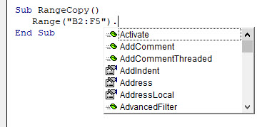
Properties will show up with the small ‘hand’ icon, while methods will show up with the small green ‘block’ icon.
Select Method
One of the most common methods to use is the select method. This enables use to select specific cells or a cell in the Excel worksheet.
To select a single cell in a worksheet, we can just refer to the single cell in the Worksheet.Range Object
Sub SelectRange
  Worksheets("Sheet1").Range("B2").Select
End Sub
To select a range of cells, we can refer to a range of cells in the Worksheet.RangeObject.
Sub SelectRange
  Worksheets("Sheet1").Range("B2:C5").Select
End Sub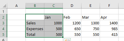
To select 2 non-contiguous ranges, we can use a comma between 2 ranges.
Sub SelectWorksheetRange
 Worksheets("Sheet1").Range("B3:B5, C2:F2").Select
End Sub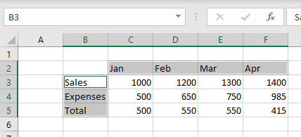
Copy and PasteSpecial Methods
We can copy the information from cells to other cells using the Copy and PasteSpecial Methods.
Sub WorksheetRangeCopy()
  Worksheets("Sheet1").Range("B2:F5").Copy
  Worksheets("Sheet1").Range("B8").PasteSpecial xlPasteAll
End Sub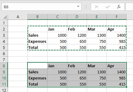
Font Property
We can use the Font Property to format the cells. In the example below, we are using the Bold property of the Font Property to bold the cells.
Sub WorksheetRangeFont()
  Worksheets("Sheet1").Range("B3:B5, C2:F2").Font.Bold = True
End Sub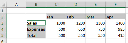
Borders Property
We can use the Borders Property, and then the LineStyle property of the Borders property to put borders around all the cells.
Sub WorksheetRangeCopy()
 Worksheets("Sheet1").Range("B2:F5").Borders.LineStyle = xlContinuous
End Sub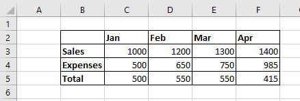
VBA Coding Made Easy
Stop searching for VBA code online. Learn more about AutoMacro — A VBA Code Builder that allows beginners to code procedures from scratch with minimal coding knowledge and with many time-saving features for all users!

Learn More
CurrentRegion Property
We can use the Current Region property of the Range object, and then the Select Method of the Current Region object to select all cells that are within the current region of the specified cell.
The current Region will select all the cells that are adjacent to the cell that is specified in the Range as long as those cells are contiguous. It will not select any cells after a blank row or column.
Sub CurrentRegion()
 Worksheets("Sheet1").Range("B2").CurrentRegion.Select
End Sub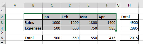
UsedRange Property
If we want to select all the cells that are populated in a worksheet, we need to use a Property of the Worksheet itself called UsedRange.
Sub UsedRangeSelect()
  Worksheets("Sheet1").UsedRange.Select
End Sub