What is a user interface in excel

The ribbon, tabs, commands gridlines, control buttons, etc. that a user can see and interact with on the screen after opening an Excel spreadsheet are called User Interface Environment in MS Excel.

Excel is an electronic spreadsheet program, developed by Microsoft Corporation.  An Excel Spreadsheet is used to record, validate and analyze the numeric data for maintaining Payrolls, Selling and purchasing product orders, Progress Reports, family budgets, and more.

These are calculated whether using general, financial, logical, statistical, engineering or other functions and formulas. The features in the excel environment are explained below in the screenshot.

Quick Access Toolbar:

The Quick Access Toolbar appears at the top left corner of the Excel application and other MS Office suites. The default commands of the Quick Access Toolbar are Save, Undo and Redo.

In the graphical user interface environment in MS Excel, the File menu is also known as the File Tab, used to control and access the file functions of the MS Office suite.

Officially, it handles files using the file menu commands such as new, open, save, save, print, share, export, publish, close, account and options. To read the File menu features in an Excel environment click here.

Tell me:

In the user interface of Microsoft Excel, the tell me to search box helps you search the command quickly and easily without going to the ribbon tab or group. Here you can type any command name you want to use or apply to the Sheet/Document. 

Title Bar:

You can see the title bar at the top of the excel spreadsheet application (MS Office suites) with the name currently being used. The name of the workbook appears in the middle of the title bar. The name of the workbook here we called is a title.

Sign in:

Microsoft’s free account is used to purchase, activate, and access Microsoft services. You can save and receive your documents from anywhere using the service. You can also use this account to use and access OneDrive, Skype, and Microsoft store.

This option appears at the top right corner, underneath the close button, you can save your work on different platforms by sharing with caring. These Platforms are Google Cloud, One Drive, E-mail, Blogs, people, etc.

Control Buttons:

The Minimize, Restore Down/Maximize and Close buttons are called Control Buttons. These appear at the top right corner of the (MS Office Suite of Applications) Excel Spreadsheet.

Ribbon:

The Ribbon is a collection of groups, commands and functions and locates under each Tab such as Home, Insert, Design, Layout, References, Mailings, Review and View, It is designed to help you quickly and easily find the groups and commands to complete a task you want.

Ribbon Display Options:

The Ribbon Display options are located at the right corner of the title bar and the 4th position on the left of the Control buttons.  The Ribbon Display Options include Auto-Hide Ribbon, Show Tabs, Show Tabs and Commands. 

Tabs:

Home, Insert, Page Layout, Formulas, Data, Review, and view are called Tabs. Each tab is a form of group. Similarly, each Group is a form of the command.

Groups:

Each tab is a form of group. Similarly, each group is a form of the command. For example, Groups on the Home tab include Clipboard, Font, Alignment, Number, Style, Cells, and Editing.

Commands

A command is part of a group. And access to a specific piece of work. For example, the Font group commands include bold, italic, underline, etc.

Name Box:

It is the reference (address) for a specific cell or range of cells or you can set the name for a particular cell or range of cells in an excel spreadsheet.

Insert Functions:

It helps to get the result by using a particular function based on its arguments. This is one of the features of Excel.

Formula bar:

In the Formula bar, you can view and modify the function or formula that applies to any cell in the sheet for any calculation.

Row and Column Headings:

The column is a collection of Vertical light grey coloured lines containing the letters used to identify each column in a worksheet.

The column heading appears on the top of it (above the first row). The row is a collection of Horizontal light grey coloured lines containing the number used to identify each row in a worksheet. The Row Heading appears at the beginning of it (left of the first column).

Without Row and Column Headings in excel you cannot perform an autofill feature.

Vertical/Horizontal Scrollbar:

The scrollbar is used to view the worksheet in any part by using the Vertical or Horizontal scrollbar whether by moving up, down, left or right.

Page View Options:

Page View Options appear at the right but one on the taskbar. These are

Normal: Normal is a default view and is easier to work in this mode in the worksheet.

Page Layout: In the Page Layout mode, the worksheet is divided into more page sizes for print preview.

Page Break Preview: The Page Break Preview shows the worksheet as separate pages where there are the contents to see how a page look likes.

Zoom Slider/Toolbar:

To zoom in and out excel spreadsheet in the desired size, use the Zoom slider, which appears at the bottom right corner of the workbook.

Click to Select All:

Click on the top left of the common area (Under the Name Box) of the Column and Row Headings to select the entire worksheet. Just like Ctrl + A.

Gridlines:

The Gridlines are the collection of Horizontal and Vertical light grey coloured lines in a worksheet.

Cell in Excel:

In the Microsoft Excel Spreadsheet Environment, A cell is an Intersection of Rows and columns to form like a rectangle in a worksheet.

Cell Address:

The location of a cell is identified by its column letter and the row number is called, cell address or cell reference.

Active Cell:

An Active Cell in the graphical user interface is where it is bold with a dark outline. An Active cell is an identifiable mark that can be accepted to enter and edit the content.

Active Sheet/sheet tab:

For a selected worksheet that is currently being used, the name of the sheet tab is in bold and appears at the bottom left corner of the workbook.

Range of cells:

In the Microsoft Excel Spreadsheet Environment, More than two cells that are selected horizontally or vertically are called a range of cells.

Sheet tabs:

In the user interface environment in MS Excel, The name of the sheets that appears from the bottom left corner of the worksheet are called sheet tabs.

Insert New Worksheet:

To insert more worksheets in a workbook, click the insert sheet tab button, located right to the sheet tabs.

Excel Interface Components

Excel has two main UI components: The Interface Components and the Workbook Components. In this blog post, you will learn how to identify the Excel Interface Components.

Interface Components

The interface components of Excel include the Quick Access Toolbar, Ribbon, Name Box, Formula Quick Menu, Formula Bar, Status Bar, Worksheet View Options, Zoom Slider Control, and the Zoom Percentage Indicator.

Quick Access Toolbar

The Quick Access Toolbar is found on the top-left of the Excel window which contains the commonly-used commands in Excel. This toolbar can be customized and lets you choose which commands you want to access easily. By default, this contains the save, undo, and redo commands.

Ribbon

The Ribbon interface contains the commands that are available for use in Excel. This has multiple tabs including the File, Home, Insert, Page Layout, Formulas, Data, Review, View, Add-ins, and Help tabs. There are tabs that will appear when necessary; for example, the Format tab appears when you click an inserted shape.

The tabs are then subdivided in groups based on the usage of the commands. For example, in the Home tab, the commands are grouped in Clipboard, Font, Alignment, Number, Styles, Cells, and Editing.

Name Box

The Name Box is an input box which normally displays the name or location of the active cell on the worksheet. This is also used to directly create a named range. When you open a blank workbook, the selected cell is A1, by default.

Formula Quick Menu

The Formula Quick Menu beside the Name box is a shortcut when you want to insert a function. If you click the fx option, the Insert Function will pop-up to let you choose which Excel function would you like to use.

Formula Bar

The Formula Bar is found just beside the Formula Quick Menu. This allows you to enter or edit data, formula or a function that will appear in the selected cell whose name or location appears in the Name Box.

Status Bar

The Status Bar in the bottom-left corner of the Excel window displays various information about the current mode of the workbook.

Worksheet View Options

The Worksheet View Options lets you choose which of the 3 worksheet views you want (Normal, Page Layout, or Page Break Preview). By default, the worksheet view is set to Normal.

Zoom Slider Control

The Zoom Slider Control helps you zoom in and zoom out the worksheet.

Zoom Percentage Indicator

The Zoom Percentage Indicator displays the zoom percentage just beside the Zoom Slider Control. By default, it is set to 100%.

The rectangular grid of rows and columns described in Excel Spreadsheets is only one part of the Excel user interface. The entire interface is as follows:

Figure 1 – Excel User Interface

This is the layout used in Excel 2007. The layout in Excel 2010 and Excel 2013 and later versions of Excel are almost identical. The key components are as follows:

Title Bar – contains the name of the workbook. The default is Book1 (and then Book2, etc.). This is replaced by the filename once the Excel workbook is saved.

Worksheet Tabs – a list of all the worksheets in the workbook. By default, these are labeled Sheet1, Sheet2, etc. You can navigate to any worksheet in the workbook by clicking on that worksheet tab. You can also use the four small arrows  to the left of the worksheet tabs for navigation purposes. The first arrow is used to go to the first worksheet, the second to go to the previous worksheet, the third to go to the next worksheet and the fourth to go to the last worksheet. You can change the name of any of the worksheets by doubling clicking on its tab and then entering a new name. You can add a new worksheet by clicking on the rightmost worksheet tab icon . You can also change the order of the worksheets in the list by left-clicking on a worksheet tab and dragging it to a new location in the list. You can access other capabilities by right-clicking on any of the worksheet tabs or the worksheet tab arrows.

Ribbon Tabs – the top-level menu items. In the example above this consists of Home, Insert, Page Layout, Formulas, etc. The actual choices can change depending on the state that you are in. To access most capabilities in Excel you click on one of these ribbon tabs. For each tab, a different ribbon will be displayed. In Figure 1 the Home ribbon is displayed. This tab provides access to the most common Excel capabilities.

Ribbon – a collection of Excel capabilities organized into groups corresponding to some ribbon tab. For example, the Home ribbon displayed in Figure 1  is organized into the Clipboard, Font, Alignment, Number, etc. groups. Each group consists of one or more icons corresponding to some capabilities in Excel. For example, to center the content of a cell in a worksheet, click on that cell and then click on the center icon  in the Alignment group on the Home ribbon. We use the following abbreviation for this sequence of steps: Home > Alignment|Center.

In a similar manner, you can merge two neighboring cells by highlighting the two cells and selecting Home > Alignment|Merge & Center; the two cells are combined and any content placed in the merged cell will be centered. Also, cells, rows, columns, and worksheets can be inserted, deleted, and formatted using Home > Cells.

There are also shortcuts for some icons. E.g., to center the contents of a cell, you can click on that cell and then enter Ctrl-E.

To get some idea of the purpose of an icon, place the mouse pointer over that icon (without clicking) and a tooltip will appear to provide some information about the icon.

Some of the groups on a ribbon are accompanied by a small arrow (to the right of the name of the group). When you click on this arrow you will be presented with a dialog box that provides you with various options to choose from. E.g. clicking on the arrow for the Font group on the Home ribbon brings up a dialog box with tabs labeled Number, Alignment, Font, Border, etc. Each tab in the dialog box presents you with a different set of options for formatting the range of cells that are currently highlighted in the worksheet. For example, to specify that you want numbers in the highlighted cells to be displayed with 3 decimal places, you select the Number tab and then the Number option and finally fill in 3 in the box specifying the number of decimal places.

Some icons within a group are also accompanied by a small downward arrow. When you click on this arrow you will be presented with a vertical list of options. E.g. clicking on the Insert icon in the Cells group in the Home ribbon brings up the choices Insert Cells…, Insert Sheet Rows, Insert Sheet Columns, Insert Sheet.

Some groups also contain scrollable drop-down lists accompanied by a downward arrow. E.g. clicking on the arrow to the right of the Font drop-down list in the Font group on the Home ribbon, presents a scrollable list of available fonts (Arial, Time New Roman, etc.) to choose from.

Office Button – the icon in the upper left side of the Excel 2007 interface that allows you to open, save and print workbooks. When you click on this icon you will be presented with a menu of options. In addition to opening, saving and printing workbooks, there is a button called Excel Options. Clicking on this button displays a dialog box that offers you the ability to change various configuration parameters.  It also contains the Add-In option that we will describe later.

Excel 2010 and later versions of Excel do not use the Office Button. Instead, they provide the same functionality using the File tab. The File tab is the first ribbon tab in versions of Excel starting with Excel 2010 and is located to the left of the Home tab.

Quick Access Toolbar – contains frequently used icons and is located in the upper left-hand corner of the display (just to the right of the Office Button in Excel 2007 and above the File and Home tabs in versions of Excel starting with Excel 2010). Initially, the toolbar contains the Save, Repeat and Undo icons. You can add or delete icons from this toolbar by clicking on the small downward arrow at the right end of the toolbar to display a customization dialog box.

Active Cell – displays the currently referenced cell. This is the cell that you last clicked on with the mouse or moved to. This cell is highlighted on the display.

Name Box – contains the address of the active cell. You can navigate to another cell simply by entering the address of that cell in the Name Box and pressing the Enter key.

Formula Bar – contains the contents of the active cell. When this is a formula, the formula appears here while the value of the formula appears in the cell. You can optionally click on the f_x symbol located just to the left of the Formula Bar to bring up a dialog box that helps you find the appropriate function as well as the arguments for this formula.

Vertical/Horizontal Split Controls – used to split the worksheet. The vertical split control is a small rectangular box located just above the vertical scroll bar. If you move the control downward, the display of the worksheet splits in two so that you can see two different parts of the worksheet at the same time. If you move the control back to its original position the two parts reunite and only one view of the worksheet is displayed.

The horizontal split control is located just to the right of the horizontal scroll bar and works in a similar manner. If you move the control to the left the worksheet display splits horizontally into two parts.

Status Bar – contains certain information, including by default the sum, count and average of any highlighted range. It also contains the zoom and zoom slider, which are used to increase or decrease the size of the worksheet display. You can customize what information appears on the status bar by right-clicking on it to display a customization dialog box.

What is user interface in Excel?

The rectangular grid of rows and columns described in Excel Spreadsheets is only one part of the Excel user interface. The entire interface is as follows: Figure 1 – Excel User Interface. This is the layout used in Excel 2007.

How do I run code in Excel?

Is Excel macros easy to learn?

Before you get intimidated and write macros off as yet another Excel feature that’s far too complex and advanced for you, take a breath. The concept of a macro might seem complicated. But, learning to use them to your advantage is actually surprisingly simple.

What are the steps to run a macro?

How much time does it take to learn macros?

So, if you need to create basic macros, you can just learn basic syntax and start coding in about 2 hours. If however, you wish to create complicated programs, you would require to know about all the Excel formulas and how they work as well. That might take up to 1 month.

How do I write a VBA macro?

What is macro in Excel with example?

Excel Macro is a record and playback tool that simply records your Excel steps and the macro will play it back as many times as you want. VBA Macros save time as they automate repetitive tasks. It is a piece of programming code that runs in an Excel environment but you don’t need to be a coder to program macros.

What is macro example?

A macro is like an algorithm or a set of actions that we can use or run multiple times. A macro helps in automating or repeating tasks by recording or storing our input sequences like mouse strokes or keyboard presses. Once this input is stored, it makes up a macro which is open to any possible changes.

What is VBA used for?

VBA is used to automate tasks and perform several other functions beyond creating and organizing spreadsheets. For example, users require to automate some aspects of Excel, such as repetitive tasks, frequent tasks, generating reports, etc.

Which is better VBA or python?

Unlike the VBA language used in Excel, data analysis using Python is cleaner and provides better version control. Better still is Python’s consistency and accuracy in the execution of code. Other users can replicate the original code and still experience a smooth execution at the same level as the original code.

Is VBA difficult to learn?

The Visual Basic for Applications (VBA) programming language allows you to automate routine tasks in Excel—and it’s not as hard to learn as most people think. Programming techniques are demonstrated through real-world examples.

Is VBA worth learning?

VBA is worth learning if you plan to work mostly with MS-office programs and want to automate the Excel process and exchange data to and from Office applications. If you want to focus on a broader work environment, other languages such as Python could be more useful.

Is VBA a dying language?

VBA is not as dead as you think.

Excel automation can also use TypeScript to create Office Scripts which can be used to automate Excel Online. In 2020, VBA still shows twice as much interest as a popular programming language that can be used to automate Excel. (The most loved programming language is Rust.

Can Python replace VBA?

Yes, absolutely! VBA is commonly used to automate Excel with macros, add new user defined worksheet functions (UDFs) and react to Excel events. Everything you would previously have done in Excel using VBA can be achieved with Python.

Интерфейс Microsoft Excel состоит из множества элементов: полей, строк, столбцов, панелей команд и т.д. Есть элементы, которые выполняют множество самых различных задач, например, многофункциональная Лента, которая занимает большую часть интерфейса. Есть элементы менее функциональные, но не менее полезные, например, Строка формул или поле Имя. В данном уроке мы изучим интерфейс Microsoft Office Excel и подробно разберем каждый из элементов.

Excel 2013 — это приложение Microsoft Office, предназначенное для работы с электронными таблицами, которое позволяет хранить, организовывать и анализировать информацию. Если у Вас сложилось мнение, что Excel используют только специалисты для выполнения сложных задач, то Вы ошибаетесь! На самом деле любой желающий может воспользоваться всеми возможностями Excel и применить всю их мощь для решения своих задач.

Интерфейс Excel

Интерфейс приложения Excel 2013 очень похож на интерфейс Excel 2010. Если Вы ранее уже работали с Excel 2010, то освоить Excel 2013 не составит большого труда. Если же Вы впервые знакомитесь с Excel или работали преимущественно с более ранними версиями, то освоение интерфейса Excel 2013 займет некоторое время.

При первом открытии Excel появится Начальный экран. Здесь Вы можете создать новую рабочую книгу, выбрать шаблон или открыть одну из последних книг.

Лента

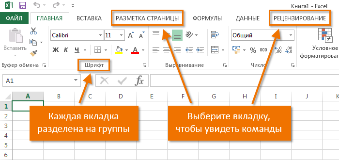
Лента является основным рабочим элементом интерфейса MS Excel и содержит все команды, необходимые для выполнения наиболее распространенных задач. Лента состоит из вкладок, каждая из которых содержит нескольких групп команд.

Панель быстрого доступа

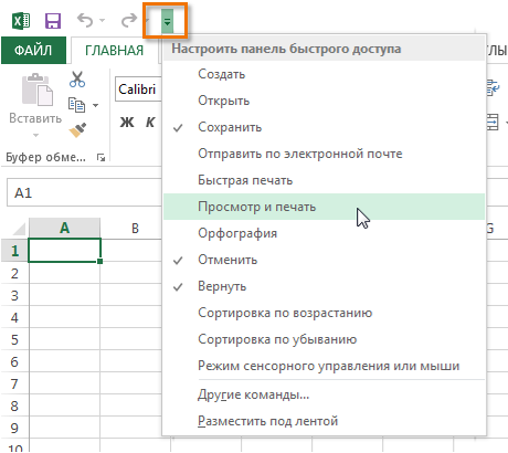
Панель быстрого доступа позволяет получить доступ к основным командам независимо от того, какая вкладка Ленты в данный момент выбрана. По умолчанию она включает такие команды, как Сохранить, Отменить и Вернуть. Вы всегда можете добавить любые другие команды на усмотрение.

Учетная запись Microsoft

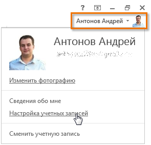
Здесь Вы можете получить доступ к Вашей учетной записи Microsoft, посмотреть профиль или сменить учетную запись.

Группа Команд

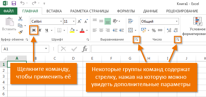
Каждая группа содержит блок различных команд. Для применения команды нажмите на необходимый ярлычок. Некоторые группы содержат стрелку в правом нижнем углу, нажав на которую можно увидеть еще большее число команд.

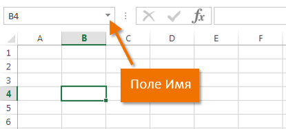
Поле Имя

В поле Имя отображает адрес или имя выбранной ячейки. Если вы внимательно посмотрите на изображение ниже, то заметите, что ячейка B4 – это пересечение столбца B и строки 4.

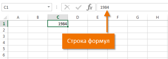
Строка Формул

В строку формул можно вводить данные, формулы и функции, которые также появятся в выбранной ячейке. К примеру, если вы выберите ячейку C1 и в строке формул введете число 1984, то точно такое же значение появится и в самой ячейке.

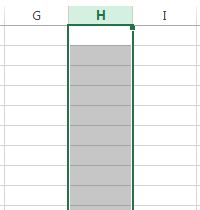
Столбец

Столбец – это группа ячеек, которая расположена вертикально. В Excel столбцы принято обозначать латинскими буквами. На рисунке ниже выделен столбец H.

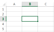
Ячейка

Каждый прямоугольник в рабочей книге Excel принято называть ячейкой. Ячейка является пересечением строки и столбца. Для того чтобы выделить ячейку, просто нажмите на нее. Темный контур вокруг текущей активной ячейки называют табличным курсором. На рисунке ниже выбрана ячейка B3.

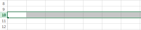
Строка

Строка – это группа ячеек, которая расположена горизонтально. Строки в Excel принято обозначать числами. На рисунке ниже выделена строка 10.

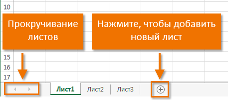
Рабочий лист

Файлы Excel называют Рабочими книгами. Каждая книга состоит из одного или нескольких листов (вкладки в нижней части экрана). Их также называют электронными таблицами. По умолчанию рабочая книга Excel содержит всего один лист. Листы можно добавлять, удалять и переименовывать. Вы можете переходить от одного листа к другому, просто нажав на его название.

Режимы просмотра листа

Существуют три основных режима просмотра листа. Для выбора необходимого режима просто нажмите соответствующий ярлычок.

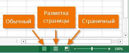
• Обычный режим выбран по умолчанию и показывает вам неограниченное количество ячеек и столбцов.
• Разметка страницы — делит лист на страницы. Позволяет просматривать документ в том виде, в каком он будет выведен на печать. Также в данном режиме появляется возможность настройки колонтитулов.
• Страничный режим – позволяет осуществить просмотр и настройку разрывов страниц перед печатью документа. В данном режиме отображается только область листа, заполненная данными.

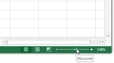
Масштаб

Нажмите, удерживайте и передвигайте ползунок для настройки масштаба. Цифры справа от регулятора отображают значение масштаба в процентах.

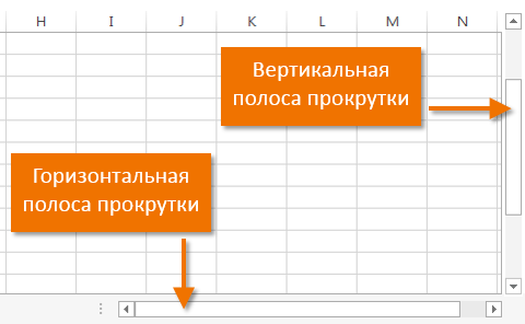
Вертикальная и горизонтальная полосы прокрутки

Лист в Excel имеет гораздо большее количество ячеек, чем вы можете увидеть на экране. Чтобы посмотреть остальную часть листа, зажмите и перетащите вертикальную или горизонтальную полосу прокрутки в зависимости от того, какую часть страницы вы хотите увидеть.