Содержание
- Series Formula
- [=SERIES(Name, X-Values, Y-Values, PlotOrder, Bubble Sizes) ]
- Series Formula Rules and Facts
- Examples of Valid Series Formula
- Changing the Arguments
- Important
- The Excel Chart SERIES Formula
- The SERIES Formula
- Series Formula Arguments
- Series Name
- X Values
- Y Values
- Plot Order
- Bubble Size
- Editing SERIES Formulas
- Cell References and Arrays in the SERIES Formula
- Normal Cell References
- Fragmented Ranges
- Ranges in Other Workbooks
- Names (Named Ranges)
- Arrays
- Using VBA with the SERIES Formula
- Edit SERIES Formulas (Find-Replace)
- More VBA & SERIES Formula Examples
- Add Names to Chart Series
- Add Series to Existing Chart
- Multiple Trendline Calculator
- Switch X and Y Values (or Axes)
- Peltier Tech Consulting Services
- Coming to You From…
- Share this:
- Reader Interactions
- Comments
- Leave a Reply
- Primary Sidebar
- Excel Charting Add-Ins
- Peltier Tech Newsletter
- Peltier Tech Training
Series Formula
A data series is just a group of related data representing a row or column from the worksheet.
When you select a particular data series on a chart its corresponding series formula will appear in the formula bar.
When the source data is changed you will see that the series formula is changed automatically.
When a series is selected the series formula is displayed in the formula bar at the top. The name of the series is displayed in the «Name box» to the left of the formula bar.
Excel uses a series formula or function to define a data series for a chart. There is one series formula for each data series.
Although this resembles a typical worksheet formula there are a few important differences.
1) The SERIES function cannot be used directly from another cell.
2) This formula cannot contain any worksheet functions.
It is possible though to edit this formula and to manually change the arguments.
Surface charts do not have series formula ?
chart types — 83,84,85,86
[=SERIES(Name, X-Values, Y-Values, PlotOrder, Bubble Sizes) ]
The data used in each series in a chart is determined by its SERIES formula. Press Enter to apply any changes.
Name — (Optional) — This is the name of the series and is displayed in the legend. If the chart has only one series this name is used as the title. This can be blank, a text string in double quotes, a reference to a worksheet range or a named range. If this is left blank, then Excel will provide a default name (Series 1, 2, 3 etc)
X-Values — (Optional) — These are the labels that are used on the category axes. If this is left blank then consecutive integers are used 1,2,3 . This can be blank, a literal array of numeric values or text labels enclosed in curly brackets , a reference to a worksheet range or a named range. It is also possible to have a non-continuous range reference. The separate ranges must be put inside a bracket and must be separated by commas (eg ??)
Y-Values — These are the values you want to plot. This can be blank, a literal array of numeric values enclosed in curly brackets , a reference to a worksheet range or a named range. It is also possible to have a non-continuous range reference. The separate ranges must be put inside a bracket and must be separated by a commas (eg ??).
PlotOrder — This is the plotting order for the data series. The Series tab displays the series in the order in which they are plotted. This is also the order in which the series names will appear in the legend. When there is only one series then this is omitted. This must be a whole number between 1 and the number of series on the chart. If you enter zero then 1 is used. If you enter a number greater than the number of series then the total number of series is used. This cannot be a cell reference.
Bubble Sizes — (Optional) — These are the values of the bubble sizes. This can be blank, a literal array of numeric values enclosed in curley brackets, a reference to a worksheet range or a named range. It is also possible to have a non-continuous range reference. The separate ranges must be put inside a bracket and must be separated by a commas (eg ??).
Series Formula Rules and Facts
Range references in a SERIES formula are always absolute and always contain a worksheet name. If you have defined named ranges then the series formula can contain a named range in place of a range.
Any range references used are always prefixed with the worksheet name.
Any range references used are always absolute references (as opposed to relative).
If you accidently remove the worksheet name or use a relative reference, these will be changed automatically.
Each data series has a corresponding series formula and the number of arguments will depend on the chart type.
Examples of Valid Series Formula
=SERIES(Name, X-Values, Y-Values, PlotOrder, Bubble Sizes)
=SERIES(Sheet1!$C$2, Sheet1!$B$3:$B$9, Sheet1!$C$3:$C$9, 1)
=SERIES(«North», <«Mon»,»Tue»,»Wed»,»Thu»,»Fri»,»Sat»,»Sun»>, <0.65,0.21,0.86,0.97,0.05,0.34,0.74>, 1)
=SERIES(Sheet1!$C$2, , Sheet1!$C$3:$C$9, 2)
=SERIES(Sheet1!$C$2, Sheet1!$B$3:$B$9, Sheet1!$C$3:$C$9, 3, Sheet1!$D$3:$D$9)
=SERIES(, (Sheet1!$B$3:$B$9, Sheet1!$B$20:$B$30), (Sheet1!$C$3:$C$9, Sheet1!$C$20:$C$30), 4)
Changing the Arguments
You can change any of the series formula arguments in four ways you can change the series name of a data series:
1) Overwriting the cell(s) which the argument refers to.
2) Using the Automatic Range Finders to move the source data.
3) Using the (Chart > Source Data)(Series tab).
4) Editing the Series Formula.
The only way to change the order of the data series is to either use the (Chart > Source Data)(Series tab) or to edit the series formula directly.
Important
Excel’s normal practice is to assume that all the series share the same X-Values in the first column or row and that each successive column or row holds the Y-data for a separate series.
Surface charts do not have series formulas.
When you create a chart that uses a named range, Excel does not automatically substitute the name in the series formula.
If you delete a named range that is used in a chart series, the invalid name will remain and the chart will not display properly.
Pie charts can only have a single series unless .
All the different parts of a series formula (except Plot Order) can be linked to a worksheet (in any workbook).
The maximum number of data points on a normal 2D chart is 32,000.
Bubble charts need three sets of values representing the x value, y value and the size of the bubbles.
You can display as many as 255 different data series on a chart (except Pie Charts).
Try to avoid having too many data series on a single chart.
You can have a chart object with no series, although I can’t see any point
There is a direct link between the chart and the worksheet containing the data. It is possible to change the underlying data in the worksheet by dragging a individual chart point to a new position.
It is important to remember that any of the parameters in the SERIES formula can be a constant, a literal arrway a reference to a worksheet range or a named range.
Источник
The Excel Chart SERIES Formula
Tuesday, September 24, 2019 by Jon Peltier 1 Comment
Data in an Excel chart is governed by the SERIES formula. This formula is only valid in a chart, not in any worksheet cell, but it can be edited just like any other Excel formula.
The SERIES Formula
Select a series in a chart. The source data for that series, if it comes from the same worksheet, is highlighted in the worksheet. And a formula appears in the Formula Bar.
You didn’t have to write the formula. Excel writes it for you when you create a chart or added a series.
The formula in the chart shown above is:
The arguments are identified as follows:
In the case of a bubble chart, there is one additional argument:
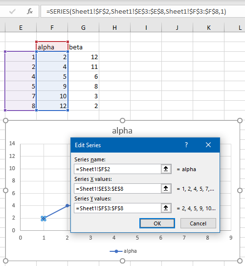
You can also view the series data using the Select Data dialog. Right click on the chart and choose Select Data, then select the series in the list and click the Edit button. The Edit Series dialog shows the same data that the SERIES formula shows.
Here are a few valid SERIES formulas. This formula has conventional cell addresses:
This formula plots the same, although the values are not linked to the worksheet, but are instead hard-coded into the formula:
This formula doesn’t even include a Series Name or Y Values, and the Y Values are represented by a Name (Named Range).
Series Formula Arguments
Series Name
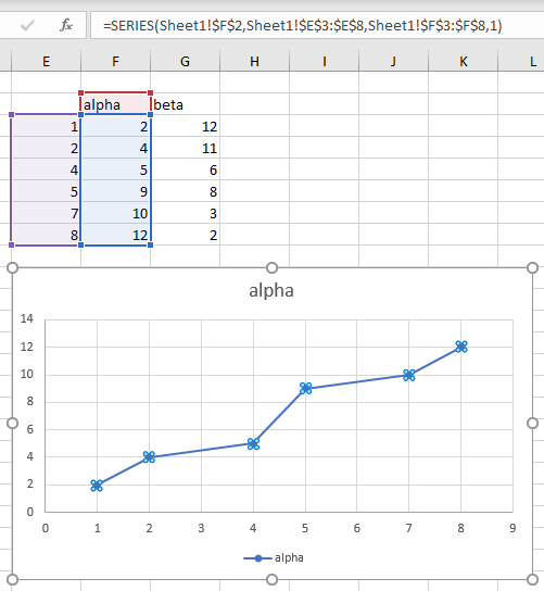
Series Name is obviously the name of the series, and it’s what is displayed in a legend. This argument is usually a cell reference, Sheet1!$F$2 , but it can also be a hard-coded string enclosed in double quotes, «alpha» , or it can be left blank. If it is blank, the series name will be “Series N“, where N is the number of the series.
X Values
X Values are the numbers or category labels plotted along the X axis (category axis) of the chart, usually the horizontal axis but the vertical axis of a horizontal bar chart. This is usually a cell reference, Sheet1!$E$3:$E$8 , but it can also be a hard-coded array in curly braces, <1,2,4,5,7,8>or <«A»,»B»,»C»,»D»,»E»,»F»>, and it can be left blank. If x Values is left blank, the series will either use the same X values as the first series in the chart uses, or it uses the counting numbers <1,2,3,etc.>. Note that in non XY Scatter charts, all series use the same X values as the first series in the chart.
Y Values
Y Values are the numbers plotted along the Y axis (value axis) of the chart, usually the vertical axis but the horizontal axis of a horizontal bar chart. This is usually a cell reference, Sheet1!$F$3:$F$8 , but it can also be a hard-coded array in curly braces, <2,4,5,9,10,12>. Y values cannot be left blank; if you try, Excel will remind you that a series must contain at least one value. A text value in the Y Values will be plotted as a zero.

Plot Order
Plot Order is a series number within the chart. This is always a number between 1 and the number of series in the chart.
“Plot Order” is a bit of a misnomer, because regardless of this number, some types of series are plotted before others. For example, all area series are plotted before all bar/column series, and those are plotted before line series, and XY scatter series are plotted last of all. Within each chart group, all primary series are plotted before all secondary series. So “Series Number” would be a better name.
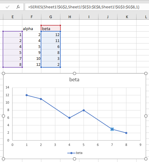
Bubble Size
Bubble Size contains the numbers used to calculate the diameters of the bubbles in a bubble chart. This is usually a cell reference, Sheet1!$G$3:$G$8 , but it can also be a hard-coded array in curly braces, <12,11,6,8,3,2>. I’ve noticed that the first element in a hard-coded array is ignored, so I pad it at the beginning with a dummy bubble size of zero: <0,12,11,6,8,3,2>. Bubble Sizes cannot be left blank; if you try, Excel will remind you that a series must contain at least one value (using the same message as for blank Y Values.
Editing SERIES Formulas
Just like any formula in Excel, you can edit the series formula right in the Formula Bar, and the new formula will change the output.
While it’s pretty easy to modify a series’ data by dragging the highlighted regions in the worksheet, you can just as easily change “F” in this series formula
to “G”, and the chart will use the series name and Y values in column G.
And both of these techniques are easier than going through the whole Select Data > Edit Series routine.
You can modify any of the arguments. You can change the series name, the X and Y values, and even the series number (plot order). You can type right in the formula, and you can use the mouse to select ranges. Just be careful not to break syntax.
You can also add a new series to a chart by entering a new SERIES formula. Select the chart area of a chart, click in the Formula Bar (or not, Excel will assume you’re typing a SERIES formula), and start typing. It’s even quicker if you copy another series formula, select the chart area, click in the formula bar, paste, and edit.
Cell References and Arrays in the SERIES Formula
Normal Cell References
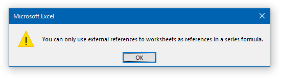
If you are referencing a cell address, you need to qualify the address with the worksheet name, Sheet1!$F$2 . If you try to enter an unqualified reference, $F$2 , Excel will give you a warning:
The SERIES formula always uses absolute references, Sheet1!$F$2 as opposed to Sheet1!F2 . If you enter a relative reference, Sheet1!F2 , Excel will automatically convert it to an absolute reference without any hassle.
Fragmented Ranges
The ranges used for X or Y Values do not need to be contiguous. The following formula is perfectly valid. Both the X Values and Y Values consist of ranges with two areas, with the two areas enclosed in parentheses.
I made use of this trick in Add One Trendline for Multiple Series, where I build an uber-formula containing data from all series in a chart (such as the formula below, for three series), and add a trendline that fits all of this data.
Ranges in Other Workbooks
A chart can reference ranges in external workbooks, as long as the ranges are properly references by workbook and worksheet.
Names (Named Ranges)
If your references are Names (Named Ranges), you need to qualify the Name with the scope of the Name, that is, either its parent worksheet or the parent workbook.
You can enter the Name qualified by the worksheet, and if the Name is scoped to the workbook, Excel will fix it for you.
Note that the Names you use in a SERIES formula cannot begin with the letters C or R (upper or lower case). You can still use these Names, but you need to use the Select Data Source/Edit Series dialogs to add them.
Arrays
When you use a hard-coded array in a SERIES formula, text values must each be surrounded by double quotes, <“D”,”E”,”F”>, while numerical values should not, <4,5,6>. If numbers are surrounded with quotes, <“4″,”5″,”6”>, they will be treated as text labels in the X Values. In an XY scatter chart, they won’t even appear in the chart, but Excel will use counting numbers <1,2,3>for X Values and zero for Y Values.
Using VBA with the SERIES Formula
Knowing how the SERIES formula works, and having a small bit of knowledge VBA, there is no shortage of charting features you can build with VBA.
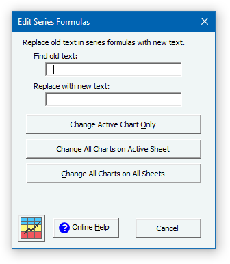
Edit SERIES Formulas (Find-Replace)
There is no built-in Find-and-Replace feature that works with SERIES formulas, but I’ve built my own. It’s based loosely on the following with a lot of error checking that I’ve had to add.
But it’s handy for changing a sheet name (e.g., Sheet1 to Sheet2 ) or column or row (column $A$ to B or row $5 to 10 ). Note that I use absolute partial references for columns and rows. Otherwise, I might want to change column S to column Q , and I’d change SERIES to QERIEQ , which would just break.
The following simple macro asks the user for two strings, one to find, and one to change to, and it changes all series in the active chart.
See How To: Use Someone Else’s Macro if you’re not sure how to implement this, or leave a comment below (I check frequently), or shoot me an email. You can modify it to work on all charts on the active sheet, or whatever you like.
This simple code, with about ten times as many lines devoted to checking for user errors and the many eccentricities of Excel, forms the basis of a popular feature in Peltier Tech Charts for Excel.
More VBA & SERIES Formula Examples
I have many more examples of VBA that uses SERIES formulas to get a certain result.
Add Names to Chart Series
Sometimes you are in a hurry to make a chart, and you don’t include the range with the series names. In Simple VBA Code to Manipulate the SERIES Formula and Add Names to Excel Chart Series I have code that determines how the data is plotted, and picks the cell above a column of Y values or to the left of a row of Y values for the name of each series in a chart.
Add Series to Existing Chart
In Add Series to Existing Chart I use VBA to find the last series in a chart, and add another series using the next row or column of data.
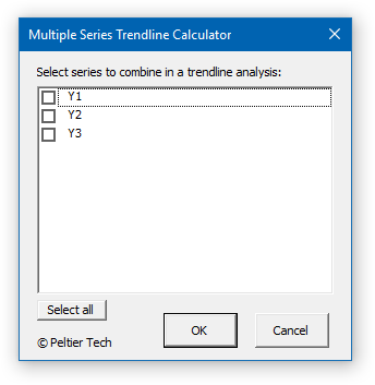
Multiple Trendline Calculator
Trendline Calculator for Multiple Series shows code that combines data from multiple series into one big series, and generates a single trendline from this larger series.
Switch X and Y Values (or Axes)
In Switch X and Y Values in a Scatter Chart, I show how to switch the X and Y components of the SERIES formula to switch the X and Y axes of a scatter chart. This is the basis of another feature in Peltier Tech Charts for Excel.

Peltier Tech Consulting Services
I enjoy doing this kind of project. Even with the ribbon components and the dialog, it only takes a few hours. And a few hours of my work will save you time every time you use the result. If you need something like this, send me your requirements and I’ll generate a quote.
Coming to You From…
Sometimes it’s easier to get into blogging from someplace that’s not my office. I used to go to a coffee shop, but that’s so cliché, and it actually doesn’t even work anymore. So today I’m writing from the newest craft brewery in Worcester, Redemption Rock. Maybe I can write it off as a business lunch!

I sampled two very nice IPAs, one very hazy, and two fine stouts, one a nitro stout that was very nice. And they have a nice concoction that combines cold-brewed coffee with the nitro stout, mmmmm.
Posted: Tuesday, September 24th, 2019 under Charting Principles.
Tags: SERIES Formula.
Comments: 1


Reader Interactions
Stefan Pinnow says
Very nice overview how a SERIES formula can look like. Replacing stuff in SERIES formula is a common task I think, at least it is for me and I have searched a long time for a proper solution. I currently use Jan Karel Pieterse’s “FlexFind” AddIn to do this. When the “Objects” checkbox is enabled it will be searched in Charts as well (as in other stuff like defined names). Then searching for e.g. “$123” will list all places where this is found. After selecting the instances from the list which one wants to replace enter the replace string, e.g. “$321” and hit replace.
In the current version (v5.3 build 596) it might happen that not all instances can be found, but you will receive a message for that. I hope that some of this instances vanish with the next release/build, because since this release there was much improvement in another AddIn of him, the “RefTreeAnalyser” which uses the same code in principle for finding stuff in SERIES formula.
Leave a Reply
This site uses Akismet to reduce spam. Learn how your comment data is processed.
Excel Charting Add-Ins

Peltier Tech Newsletter
Peltier Tech Training
Peltier Technical Services provides training in advanced Excel topics. Contact Jon at Peltier Tech to discuss training at your facility, or visit Peltier Tech Advanced Training for information about public classes.
Peltier Tech has conducted numerous training sessions for third party clients and for the public. These clients come from small and large organizations, in manufacturing, finance, and other areas.
Источник
In this video, we’ll take a closer look at data series.
When you create a chart in Excel, you’re plotting numeric data organized into one or more «data series».
A data series is just a fancy name for a collection of related numbers in the same row, or the same column.
For example, this data shows yearly sales of shorts, sandals, t-shirts, and hoodies for an online surf shop.
If I create a column chart with the default options, we get a chart with three data series, one for each year.
In this chart, data series come from columns, and each column contains 4 values, one for each product.
Notice that Excel has used the column headers to name each data series, and that these names correspond to items you see listed in the legend.
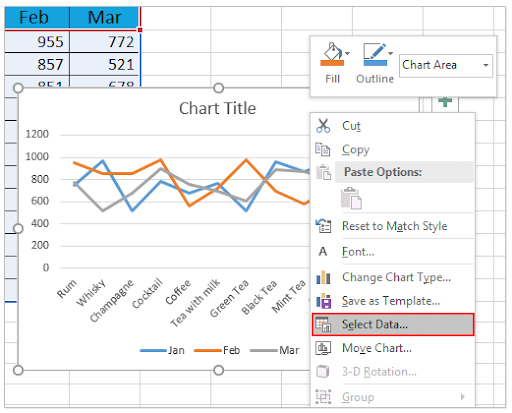
You can verify and edit data series at any time by right-clicking and choosing Select Data.
In the Select Data Source window, data series are listed on the left. If I edit one of the entries, you can see that the data series has both a name and range of values.
You’re free to edit this information manually.
So what are the values listed on the right side of Select Data Source window?
These are axis labels, in this case, Horizontal axis labels, as you can see on the chart.
In short, this chart pulls data series names from columns, and axis labels from rows.
If I click the Switch Row/Column button, this is reversed.
The data series now come from rows and axis labels come from columns.
Again, notice the legend lists data series names.
Finally, I want to point out that when you select a data series, you’ll see formula in the formula bar. This formula is based on the SERIES function, which takes four arguments:
=SERIES([Series Name],[X Values],[Y Values],[Plot Order])
As I select each series, you can see these arguments change to match the data highlighted on the worksheet.
You can edit the SERIES formula if you like. For example, if I change plot order for the shorts data series to 4, Excel automatically plots the series last, and adjusts the order of the other series automatically.
Usually, when you create a chart in Excel, it names the data series automatically. But there are some cases when you may want to change or rename the Excel Worksheet series.
By default, the names of data series in Office apps are linked to the worksheet data that are used for the chart. If you make changes to that data, they’re automatically shown in the chart.
The process of renaming or changing the series name should not be difficult as you will learn in this how to change series name in Excel article.
How to rename a data series in Excel
If you want to give you data series in Excel a new name or change the values without changing the worksheet’s data, here’s what to do:
- Open your Excel Sheet/chart that you want to rename
- Right-click the chart
- On the menu displayed, click Select Data.

- Locate the Select Data Source dialog box, then navigate to under Legend Entries (Series)
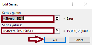
- In the Legend Entries, select the data series you want to rename, and click Edit.

- In the Edit Series dialog box, clear series name, type the new series name in the same box, and click the OK.

- The name you typed (new name) appears in the chart legend, but won’t be added to the Excel worksheet.
- Note: you can link the series name to a cell if you clear the original series name and select the specified cell, and then click the OK.

- Return to the Select Data Series dialog box, and click the OK button to save the changes. This will change the name of the specified data series.


How to Change Series Value in Excel
To change the data range for the data series, you will follow the same process, except instead of changing the Series Name, you’ll change the Series Values in the Edit Series dialogue box.
- Locate the Series values box
- Type the data range for the data series or enter the values you want.
- Click Ok
Note: again, the values you type will appear in the chart, but won’t be added to the worksheet.
Wrapping Up
In this guide to changing Series Name in Excel, we’ve discussed how to change series names in Excel and how to change seres value in Excel. We believe it has been an insightful learning opportunity.
Are you looking for more guides or want to read more Excel and tech-related articles? Consider subscribing to our newsletter here below, where we regularly publish tutorials, news articles, and guides.
Recommended Articles
You may also like to learn more about Excel in the following articles
- How to use the NPER Function in Excel
- The Most Useful Excel Keyboard Shortcuts
- How to Calculate Break-Even Analysis in Excel
- Z Score in Excel
In this tutorial, we will explore and dig up more ideas regarding how to add, change, and remove data series in Excel from your chart. Working in Microsoft Excel, whether with sales-related worksheets or not, can be time-consuming.
Consequently, we will give you a quick and easy way to add, change or rename, and remove data series in your Excel spreadsheet effectively. Excel is a big help for everybody because it makes our lives more comfortable, easy, time-saving, and convenient.
What is Data Series in Excel?
A data series is composed of cumulative and related data that is represented in rows and columns of numbers or consecutive values that are plotted in a chart. You can plot one more data series in your chart.
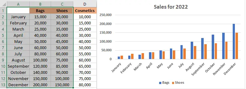
After creating a chart, you might need to add an additional data series to the chart. Refer to the illustration below.
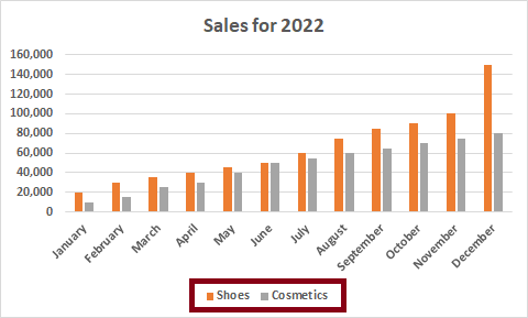
In this example, the chart shows whole-year sales data from January up to December for bags and shoes. Then, we just added a new data set to the worksheet, which is “cosmetics.”
Note: The cosmetics data series does not yet appear in the worksheet.
This is a step-by-step guide on how to get the above result.
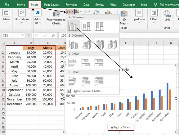
- Highlight or select all the data you want to display in the chart.
- Click the Insert tab.
- In the charts group, click the “insert column or bar graph.”
- It will automatically display the result.
Now, let’s proceed on “how to add data series to a chart in Excel.” In this result, the same procedure is applied.
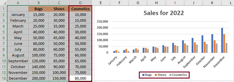
The picture above is the updated chart, in which we have already included “cosmetics.” The chart is updated automatically and displays the new data set that you added.
How to change or rename a data series name in Excel
If you want to rename or change a data series in Excel with an existing data series, or if you just want to change the values without changing the data on the worksheet, just execute the following steps:
1. Right-click the chart that contains the data series you want to change or rename.
2. Then, click “select data,” and the data source will automatically pop up.
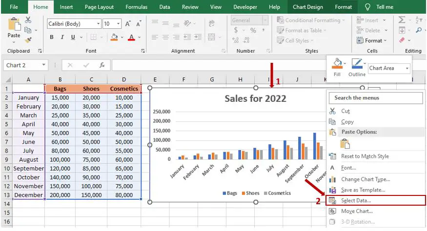
Result:
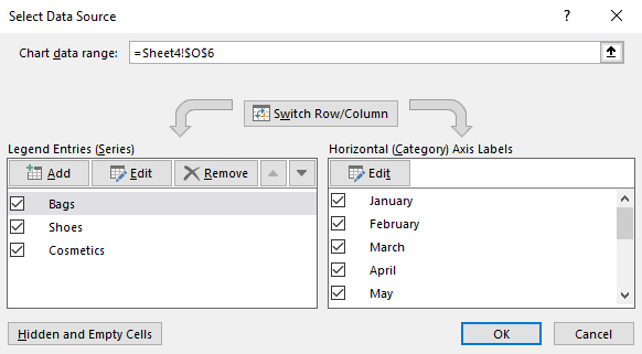
3. After you select data, in the Select Data Source dialog box, under Legend Entries (Series), select the data series and click Edit.
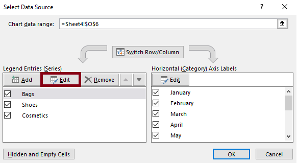
4. In the series name box, type the data you want to use, then click “OK.”
The illustrations show that “bags” were changed or renamed into “accessories.”
Result:
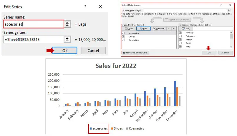
Note: The name you type will display in the chart, but it won’t be changed in the worksheet.
How to remove data series from the chart in Excel?
The procedure for removing a data series from an Excel chart was likely the same as for renaming or changing the data of a data series in Excel. However, the difference is that you have to click the “remove button.”
- Right-click the chart that contain of the data series.
- Click select data and click remove.
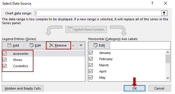
It will automatically be removed once you click “Remove.”
Result:
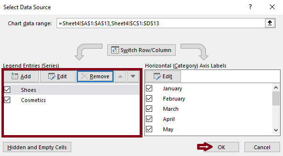
When you click “OK,” it will appear in the chart automatically. The data set has been removed, which is the “accessories.”
Note: The data you remove will no longer display in the chart, but it won’t be changed in the worksheet.
Conclusion
In this tutorial, you found the easy way on how to add, change or rename, and remove data series from the chart in Excel.
I hope all of the steps and guide mentioned above on how to add, change, and remove data series from the chart will help you and that you will apply them to your Excel spreadsheets in a more productive way.
Thank you very much for continuing to read until the end of this article. In case you have more questions, feel free to comment. You can also visit our website for additional information.
Return to Charts Home
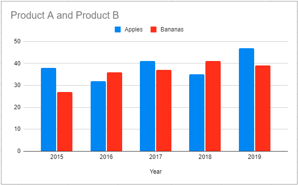
This tutorial will demonstrate how to change Series Names in Excel and Google Sheets.
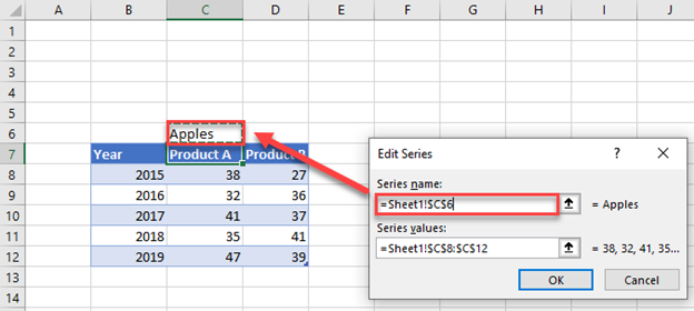
Change Chart Series Name in Excel
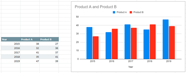
Start with your Graph
In this tutorial, we’ll show a Bar Graph comparing items sold for two different products by month. Let’s say instead of showing Product A and Product B on the graph, you want to show the actual series on the graph.
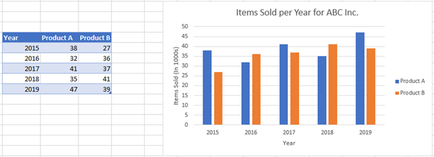
Changing Series Name
- Right click on the graph
- Click Select Data
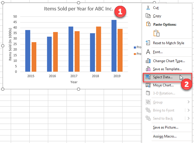
Note: You will see the Series (Product A and Product B), which correlate to the legend on the graph.
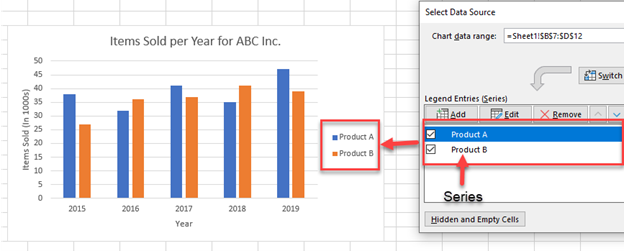
3. For each Series, Click Edit
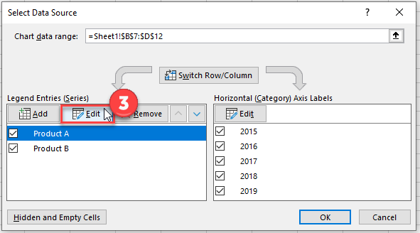
Note: You can see right now it is linked to a current cell. Right now, it is linked to “Product A”
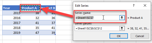
4. You can change this formula and link it to another cell
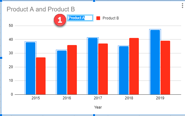
Final Graph with Series Name Change
After changing both Series Names, the final graph should look like this.
Change Chart Series Name in Google Sheets
Similar to Excel, you can see the graph with the generic series names on the graph and a table
- To Change, Double Click on the Legend Name and make your changes for both
Final Graph with Changes
As you can see, the final graph shows the updates with the new series names.