
Excel 2021 for Mac Excel 2019 for Mac Excel 2016 for Mac Excel for Mac 2011 More…Less
Do any of the following.
-
In the column, type the first few characters for the entry.
If the characters that you type match an existing entry in that column, Excel presents a menu with a list of entries already used in the column.
-
Press the DOWN ARROW key to select the matching entry, and then press RETURN .
Notes:
-
Excel automatically completes only those entries that contain text or a combination of text and numbers. Entries that contain only numbers, dates, or times are not completed.
-
Entries that are repeated within a row are not included in the list of matching entries.
-
If you don’t want the entries that you type to be matched automatically to other entries, you can turn this option off. On the Excel menu, click Preferences. Under Formulas and Lists, click AutoComplete
 , and then clear the Enable AutoComplete for cell values check box.
-
 , and then clear the Enable AutoComplete for cell values check box.
-
Select the cells that contain the data that you want to repeat in adjacent cells.
-
Drag the fill handle
over the cells that you want to fill.Note: When you select a range of cells that you want to repeat in adjacent cells, you can drag the fill handle down a single column or across a single row, but not down multiple columns and across multiple rows.
-
Click the Auto Fill Options smart button
, and then do one of the following:To
Do this
Copy the entire contents of the cell, including the formatting
Click Copy Cells.
Copy only the cell formatting
Click Fill Formatting Only.
Copy the contents of the cell, but not the formatting
Click Fill Without Formatting.
 over the cells that you want to fill.
 , and then do one of the following:
Notes:
-
To quickly enter the same information into many cells at once, select all of the cells, type the information that you want, and then press CONTROL + RETURN . This method works across any selection of cells.
-
If you don’t want the Auto Fill Options smart button
to display when you drag the fill handle, you can turn it off. On the Excel menu, click Preferences. Under Authoring, click Edit , and then clear the Show Insert Options smart buttons check box.
 , and then clear the Show Insert Options smart buttons check box.
Excel can continue a series of numbers, text-and-number combinations, or formulas based on a pattern that you establish. For example, you can enter Item1 in a cell, and then fill the cells below or to the right with Item2, Item3, Item4, etc.
-
Select the cell that contains the starting number or text-and-number combination.
-
Drag the fill handle
over the cells that you want to fill.Note: When you select a range of cells that you want to repeat in adjacent cells, you can drag the fill handle down a single column or across a single row, but not down multiple columns and across multiple rows.
-
Click the Auto Fill Options smart button
, and then do one of the following:To
Do this
Copy the entire contents of the cell, including the formulas and the formatting
Click Copy Cells.
Copy only the cell formatting
Click Fill Formatting Only.
Copy the contents of the cell, including the formulas but not the formatting
Click Fill Without Formatting.
Note: You can change the fill pattern by selecting two or more starting cells before you drag the fill handle. For example, if you want to fill the cells with a series of numbers, such as 2, 4, 6, 8…, type 2 and 4 in the two starting cells, and then drag the fill handle.
You can quickly fill cells with a series of dates, times, weekdays, months, or years. For example, you can enter Monday in a cell, and then fill the cells below or to the right with Tuesday, Wednesday, Thursday, etc.
-
Select the cell that contains the starting date, time, weekday, month, or year.
-
Drag the fill handle
over the cells that you want to fill.Note: When you select a range of cells that you want to repeat in adjacent cells, you can drag the fill handle down a single column or across a single row, but not down multiple columns and across multiple rows.
-
Click the Auto Fill Options smart button
, and then do one of the following:To
Do this
Copy the entire contents of the cell, including the formulas and the formatting, without repeating the series
Click Copy Cells.
Fill the cells based on the starting information in the first cell
Click Fill Series.
Copy only the cell formatting
Click Fill Formatting Only.
Copy the contents of the cell, including the formulas but not the formatting
Click Fill Without Formatting.
Use the starting date in the first cell to fill the cells with the subsequent dates
Click Fill Days.
Use the starting weekday name in the first cell to fill the cells with the subsequent weekdays (omitting Saturday and Sunday)
Click Fill Weekdays.
Use the starting month name in the first cell to fill the cells with the subsequent months of the year
Click Fill Months.
Use the starting date in the first cell to fill the cells with the date by subsequent yearly increments
Click Fill Years.
Note: You can change the fill pattern by selecting two or more starting cells before you drag the fill handle. For example, if you want to fill the cells with a series that skips every other day, such as Monday, Wednesday, Friday, etc., type Monday and Wednesday in the two starting cells, and then drag the fill handle.
See also
Display dates, times, currency, fractions, or percentages
Need more help?
You can always ask an expert in the Excel Tech Community or get support in the Answers community.
Need more help?
A data series is a row or column of numbers that are entered in a worksheet and plotted in your chart, such as a list of quarterly business profits. Charts in Office are always associated with an Excel-based worksheet, even if you created your chart in another program, such as Word.
Contents
- 1 How do I find the data series in Excel?
- 2 How do you create a series in Excel?
- 3 How do I add a data series to an Excel chart?
- 4 What is a data series in Excel quizlet?
- 5 What is data series?
- 6 What is Excel series?
- 7 How do you create a number data series?
- 8 What are the two ways to generate a user defined series in Excel?
- 9 What is data series Short answer?
- 10 What is chart and diagram?
- 11 Which one of these charts has only one data series?
- 12 What function converts a value to uppercase?
- 13 What is a group of data points called?
- 14 What is Series 1 Excel?
- 15 How do you name a data series in Excel?
- 16 What is a series on a chart?
- 17 How do I repeat a series of numbers in Excel?
- 18 How do you add multiple series in Excel?
- 19 Which option of the Fill Series generates a series?
- 20 How does a Vlookup work?
How do I find the data series in Excel?
You can verify and edit data series at any time by right-clicking and choosing Select Data. In the Select Data Source window, data series are listed on the left. If I edit one of the entries, you can see that the data series has both a name and range of values.
How do you create a series in Excel?
Here are the steps to use Fill Series to number rows in Excel:
- Enter 1 in cell A2.
- Go to the Home tab.
- In the Editing Group, click on the Fill drop-down.
- From the drop-down, select ‘Series..’.
- In the ‘Series’ dialog box, select ‘Columns’ in the ‘Series in’ options.
- Specify the Stop value.
- Click OK.
How do I add a data series to an Excel chart?
Adding a Series to an Excel Chart
- Click the chart to enable the Chart Tools, which include the Design and Format tabs.
- Click the “Design” tab, and then click “Select Data” from the Data group.
- Click “Add” from the “Legend Entries (Series)” section.
- Enter a name for the new data in the Series Name field.
A graphical representaion of data.A symbol that represents a single data point or value form the corresponding worksheet cell. Data Series. A group of related information in a column or row of a worksheet plotted on the chart.
What is data series?
A data series is a row or column of numbers that are entered in a worksheet and plotted in your chart, such as a list of quarterly business profits. Charts in Office are always associated with an Excel-based worksheet, even if you created your chart in another program, such as Word.
What is Excel series?
A data series is just a group of related data representing a row or column from the worksheet.The name of the series is displayed in the “Name box” to the left of the formula bar. Excel uses a series formula or function to define a data series for a chart.
How do you create a number data series?
To create this list follow these steps:
- Select cell D2.
- Type 1 and then press Enter.
- Select cell D3 if it is not already selected.
- Type 3 and press Enter on your keyboard.
- Select cell range D2:D3.
- Press and hold with left mouse button on the dot in the lower right corner of the selected cell range.
What are the two ways to generate a user defined series in Excel?
How to Generate a Number Series in MS Excel
- Opening Microsoft Excel.
- Choosing the Increments for the Number Series.
- Using the Fill Handle to Create the Number Series.
- Using an Excel Formula to Create a Number Series.
What is data series Short answer?
Answer: A data set is a collection of data. In the case of tabular data, a data set corresponds to one or more database tables, where every column of a table represents a particular variable, and each row corresponds to a given record of the data set in question.
What is chart and diagram?
As nouns the difference between diagram and chart
is that diagram is a plan, drawing, sketch or outline to show how something works, or show the relationships between the parts of a whole while chart is a map.
Which one of these charts has only one data series?
Pie Chart has only one data series.
What function converts a value to uppercase?
The toUpperCase() method returns the value of the string converted to uppercase.
What is a group of data points called?
Data Series: A group of related data points or markers that are plotted in charts and graphs. Examples of a data series include individual lines in a line graph or columns in a column chart. When multiple data series are plotted in one chart, each data series is identified by a unique color or shading pattern.
What is Series 1 Excel?
Note: If you create a chart without using row or column headers, Excel uses default names, starting with “Series 1.” You can learn more about how to create a chart to ensure your rows and columns are formatted properly.
How do you name a data series in Excel?
Rename a data series
- Right-click the chart with the data series you want to rename, and click Select Data.
- In the Select Data Source dialog box, under Legend Entries (Series), select the data series, and click Edit.
- In the Series name box, type the name you want to use.
What is a series on a chart?
A series is a set of data, for example a line graph or one set of columns. All data plotted on a chart comes from the series object.
How do I repeat a series of numbers in Excel?
How to repeat number sequence in Excel?
- Repeat number sequence in Excel with formula.
- Enter number 1 into a cell where you want to put the repeated sequence numbers, I will enter it in cell A1.
- Follow the cell, then type this formula =MOD(A1,4)+1 into cell A2, see screenshot:
How do you add multiple series in Excel?
Select Series Data: Right click the chart and choose Select Data from the pop-up menu, or click Select Data on the ribbon. As before, click Add, and the Edit Series dialog pops up. There are spaces for series name and Y values. Fill in entries for series name and Y values, and the chart shows two series.
Which option of the Fill Series generates a series?
Answer: Enter the first date in your series in a cell and select that cell and the cells you want to fill. In the Editing section of the Home tab, click “Fill” and then select “Series”. On the Series dialog box, the Series in option is automatically selected to match the set of cells you selected.
How does a Vlookup work?
The VLOOKUP function performs a vertical lookup by searching for a value in the first column of a table and returning the value in the same row in the index_number position. The VLOOKUP function is a built-in function in Excel that is categorized as a Lookup/Reference Function.
Содержание
- Add a data series to your chart
- Add a data series to a chart on the same worksheet
- Add a data series to a chart on a separate chart sheet
- Data Series
- Select Data Source
- Switch Row/Column
- Add, Edit, Remove and Move
- What Is A Data Series In Excel 2013?
- How do I find the data series in Excel?
- How do you create a series in Excel?
- How do I add a data series to an Excel chart?
- What is a data series in Excel quizlet?
- What is data series?
- What is Excel series?
- How do you create a number data series?
- What are the two ways to generate a user defined series in Excel?
- What is data series Short answer?
- What is chart and diagram?
- Which one of these charts has only one data series?
- What function converts a value to uppercase?
- What is a group of data points called?
- What is Series 1 Excel?
- How do you name a data series in Excel?
- What is a series on a chart?
- How do I repeat a series of numbers in Excel?
- How do you add multiple series in Excel?
- Which option of the Fill Series generates a series?
- How does a Vlookup work?
- Understanding Excel Chart Data Series, Data Points, and Data Labels
- Data Series and Other Chart Elements in Excel
- Modify Individual Data Markers
- Change the Color of a Single Column
- Highlight Data with an Exploding Pie Chart
- Add Emphasis With a Combo Chart
Add a data series to your chart
After creating a chart, you might need to add an additional data series to the chart. A data series is a row or column of numbers that are entered in a worksheet and plotted in your chart, such as a list of quarterly business profits.
Charts in Office are always associated with an Excel-based worksheet, even if you created your chart in another program, such as Word. If your chart is on the same worksheet as the data you used to create the chart (also known as the source data), you can quickly drag around any new data on the worksheet to add it to the chart. If your chart is on a separate sheet, you’ll need to use the Select Data Source dialog box to add a data series.
Note: If you’re looking for information about adding or changing a chart legend, see Add a legend to a chart.
Add a data series to a chart on the same worksheet
On the worksheet that contains your chart data, in the cells directly next to or below your existing source data for the chart, enter the new data series you want to add.
In this example, we have a chart that shows 2013 and 2014 quarterly sales data, and we’ve just added a new data series to the worksheet for 2015. Note that the chart does not yet display the 2015 data series.
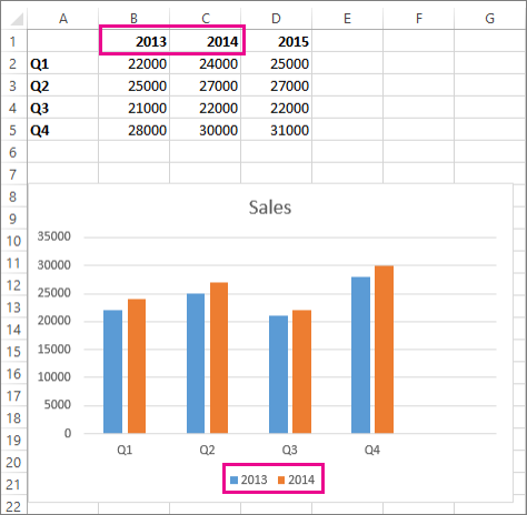
Click anywhere in the chart.
The currently displayed source data is selected on the worksheet, showing sizing handles.
You can see that the 2015 data series is not selected.

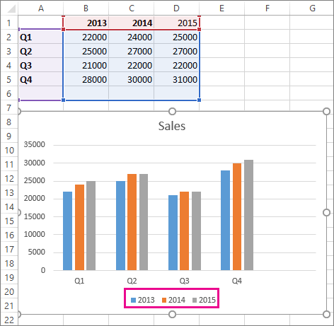
On the worksheet, drag the sizing handles to include the new data.
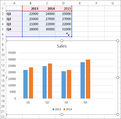
The chart is updated automatically and shows the new data series you added.
Notes: If you just want to show or hide the individual data series that are displayed in your chart (without changing the data), see:
Add a data series to a chart on a separate chart sheet
If your chart is on a separate worksheet, dragging might not be the best way to add a new data series. In that case, you can enter the new data for the chart in the Select Data Source dialog box.
On the worksheet that contains your chart data, in the cells directly next to or below your existing source data for the chart, enter the new data series you want to add.
Click the worksheet that contains your chart.
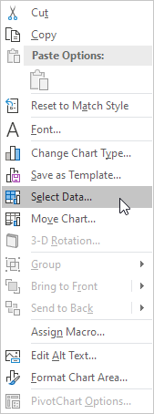
Right-click the chart, and then choose Select Data.

The Select Data Source dialog box appears on the worksheet that contains the source data for the chart.
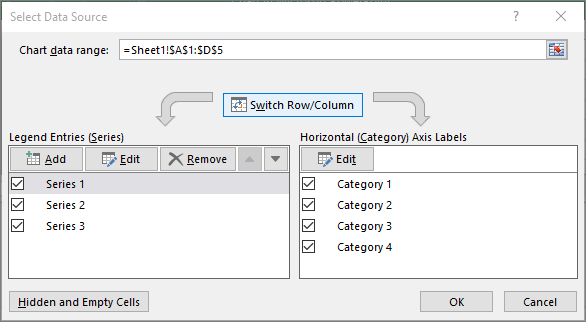
Leaving the dialog box open, click in the worksheet, and then click and drag to select all the data you want to use for the chart, including the new data series.
The new data series appears under Legend Entries (Series) in the Select Data Source dialog box.
Click OK to close the dialog box and to return to the chart sheet.
Notes: If you just want to show or hide the individual data series that are displayed in your chart (without changing the data), see:
Источник
Data Series
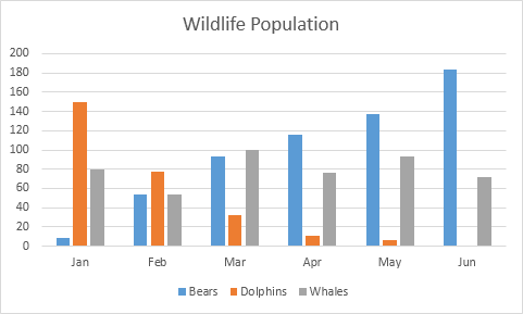
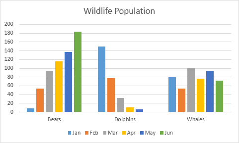
A row or column of numbers that are plotted in a chart is called a data series. You can plot one or more data series in a chart.
To create a column chart, execute the following steps.
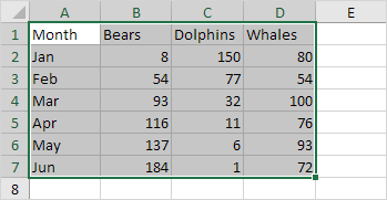
1. Select the range A1:D7.
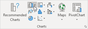
2. On the Insert tab, in the Charts group, click the Column symbol.
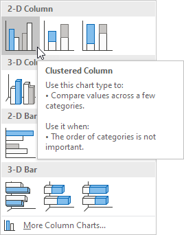
3. Click Clustered Column.
Select Data Source
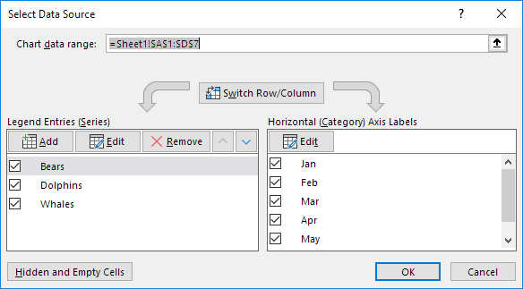
To launch the Select Data Source dialog box, execute the following steps.
1. Select the chart. Right click, and then click Select Data.
The Select Data Source dialog box appears.
2. You can find the three data series (Bears, Dolphins and Whales) on the left and the horizontal axis labels (Jan, Feb, Mar, Apr, May and Jun) on the right.
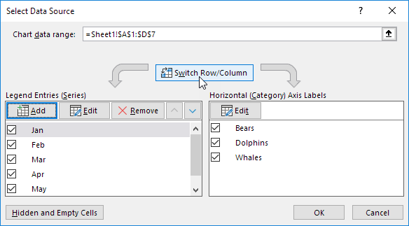
Switch Row/Column
If you click Switch Row/Column, you’ll have 6 data series (Jan, Feb, Mar, Apr, May and Jun) and three horizontal axis labels (Bears, Dolphins and Whales).
Add, Edit, Remove and Move
You can use the Select Data Source dialog box to add, edit, remove and move data series, but there’s a quicker way.
Источник
What Is A Data Series In Excel 2013?
A data series is a row or column of numbers that are entered in a worksheet and plotted in your chart, such as a list of quarterly business profits. Charts in Office are always associated with an Excel-based worksheet, even if you created your chart in another program, such as Word.
How do I find the data series in Excel?
You can verify and edit data series at any time by right-clicking and choosing Select Data. In the Select Data Source window, data series are listed on the left. If I edit one of the entries, you can see that the data series has both a name and range of values.
How do you create a series in Excel?
Here are the steps to use Fill Series to number rows in Excel:
- Enter 1 in cell A2.
- Go to the Home tab.
- In the Editing Group, click on the Fill drop-down.
- From the drop-down, select ‘Series..’.
- In the ‘Series’ dialog box, select ‘Columns’ in the ‘Series in’ options.
- Specify the Stop value.
- Click OK.
How do I add a data series to an Excel chart?
Adding a Series to an Excel Chart
- Click the chart to enable the Chart Tools, which include the Design and Format tabs.
- Click the “Design” tab, and then click “Select Data” from the Data group.
- Click “Add” from the “Legend Entries (Series)” section.
- Enter a name for the new data in the Series Name field.
What is a data series in Excel quizlet?
A graphical representaion of data.A symbol that represents a single data point or value form the corresponding worksheet cell. Data Series. A group of related information in a column or row of a worksheet plotted on the chart.
What is data series?
A data series is a row or column of numbers that are entered in a worksheet and plotted in your chart, such as a list of quarterly business profits. Charts in Office are always associated with an Excel-based worksheet, even if you created your chart in another program, such as Word.
What is Excel series?
A data series is just a group of related data representing a row or column from the worksheet.The name of the series is displayed in the “Name box” to the left of the formula bar. Excel uses a series formula or function to define a data series for a chart.
How do you create a number data series?
To create this list follow these steps:
- Select cell D2.
- Type 1 and then press Enter.
- Select cell D3 if it is not already selected.
- Type 3 and press Enter on your keyboard.
- Select cell range D2:D3.
- Press and hold with left mouse button on the dot in the lower right corner of the selected cell range.
What are the two ways to generate a user defined series in Excel?
How to Generate a Number Series in MS Excel
- Opening Microsoft Excel.
- Choosing the Increments for the Number Series.
- Using the Fill Handle to Create the Number Series.
- Using an Excel Formula to Create a Number Series.
What is data series Short answer?
Answer: A data set is a collection of data. In the case of tabular data, a data set corresponds to one or more database tables, where every column of a table represents a particular variable, and each row corresponds to a given record of the data set in question.
What is chart and diagram?
As nouns the difference between diagram and chart
is that diagram is a plan, drawing, sketch or outline to show how something works, or show the relationships between the parts of a whole while chart is a map.
Which one of these charts has only one data series?
Pie Chart has only one data series.
What function converts a value to uppercase?
The toUpperCase() method returns the value of the string converted to uppercase.
What is a group of data points called?
Data Series: A group of related data points or markers that are plotted in charts and graphs. Examples of a data series include individual lines in a line graph or columns in a column chart. When multiple data series are plotted in one chart, each data series is identified by a unique color or shading pattern.
What is Series 1 Excel?
Note: If you create a chart without using row or column headers, Excel uses default names, starting with “Series 1.” You can learn more about how to create a chart to ensure your rows and columns are formatted properly.
How do you name a data series in Excel?
Rename a data series
- Right-click the chart with the data series you want to rename, and click Select Data.
- In the Select Data Source dialog box, under Legend Entries (Series), select the data series, and click Edit.
- In the Series name box, type the name you want to use.
What is a series on a chart?
A series is a set of data, for example a line graph or one set of columns. All data plotted on a chart comes from the series object.
How do I repeat a series of numbers in Excel?
How to repeat number sequence in Excel?
- Repeat number sequence in Excel with formula.
- Enter number 1 into a cell where you want to put the repeated sequence numbers, I will enter it in cell A1.
- Follow the cell, then type this formula =MOD(A1,4)+1 into cell A2, see screenshot:
How do you add multiple series in Excel?
Select Series Data: Right click the chart and choose Select Data from the pop-up menu, or click Select Data on the ribbon. As before, click Add, and the Edit Series dialog pops up. There are spaces for series name and Y values. Fill in entries for series name and Y values, and the chart shows two series.
Which option of the Fill Series generates a series?
Answer: Enter the first date in your series in a cell and select that cell and the cells you want to fill. In the Editing section of the Home tab, click “Fill” and then select “Series”. On the Series dialog box, the Series in option is automatically selected to match the set of cells you selected.
How does a Vlookup work?
The VLOOKUP function performs a vertical lookup by searching for a value in the first column of a table and returning the value in the same row in the index_number position. The VLOOKUP function is a built-in function in Excel that is categorized as a Lookup/Reference Function.
Источник
Understanding Excel Chart Data Series, Data Points, and Data Labels
Better understand charts in Excel and Google Sheets
Charts and graphs in Excel and Google Sheets use data points, data markers, and data labels to visualize data and convey information. If you want to create powerful charts, learn how each of these elements works and how to use them properly.
Data Series and Other Chart Elements in Excel
Data Point: A single value located in a worksheet cell plotted in a chart or graph.
Data Marker: A column, dot, pie slice, or another symbol in the chart representing a data value. For example, in a line graph, each point on the line is a data marker representing a single data value located in a worksheet cell.
Data Label: Provides information about individual data markers, such as the value being graphed either as a number or as a percent. Commonly used data labels in spreadsheet programs include:
- Numeric Values: Taken from individual data points in the worksheet.
- Series Names: Identifies the columns or rows of chart data in the worksheet. Series names are commonly used for column charts, bar charts, and line graphs.
- Category Names: Identifies the individual data points in a single series of data. These are commonly used for pie charts.
- Percentage Labels: Calculated by dividing the individual fields in a series by the total value of the series. Percentage labels are commonly used for pie charts.
Data Series: A group of related data points or markers that are plotted in charts and graphs. Examples of a data series include individual lines in a line graph or columns in a column chart. When multiple data series are plotted in one chart, each data series is identified by a unique color or shading pattern.
Not all graphs include groups of related data or data series.
In column or bar charts, if multiple columns or bars are the same color or have the same picture (in the case of a pictograph), they comprise a single data series.
Pie charts are typically restricted to a single data series per chart. The individual slices of the pie are data markers and not a series of data.
Modify Individual Data Markers
When you want to call attention to a specific data marker, make it look different from the rest of the group. All you need to do is change the formatting of the data marker.
Change the Color of a Single Column
The color of a single column in a column chart or a single point in a line graph can be changed without affecting the other points in the series. A data marker that is a different color than the rest of the group will pop out on the chart.
Select a data series in a column chart. All columns of the same color are highlighted. Each column is surrounded by a border that includes small dots on the corners.
Select the column in the chart to be modified. Only that column is highlighted.
:max_bytes(150000):strip_icc()/Capture-e92aa05671d543ceaf94080eb2687619.JPG)
Select the Format tab.
:max_bytes(150000):strip_icc()/FormattabinExcel-a653a60322174f2e8ba05398723aee3e.jpg)
When a chart is selected, the Chart Tools appears in the ribbon and contains two tabs. The Format tab and the Design tab.
Select Shape Fill to open the Fill Colors menu.
:max_bytes(150000):strip_icc()/shapefill-2b9c6793611e4800a9ea6c4604b12805.jpg)
In the Standard Colors section, choose the color you wish to apply.
:max_bytes(150000):strip_icc()/StandardColors-61b542aae5d44a89a9a47f01971534f5.jpg)
Highlight Data with an Exploding Pie Chart
Individual slices of a pie chart are usually different colors. So, emphasizing a single portion or data point needs a different approach from columns and line charts. You can highlight pie charts by exploding out a single slice of pie from the graph.
Add Emphasis With a Combo Chart
Another option for emphasizing different types of information in a chart is to display two or more chart types in a single chart, such as a column chart and a line graph. You could use this approach when the graphed values vary widely or when graphing different types of data.
A typical example is a climograph or climate graph, which combines precipitation and temperature data for a single location on one chart. Additionally, combination or combo charts are created by plotting one or more data series on a secondary vertical or Y-axis.
Источник
What is a Data Series in Excel?
A data series is a collection of consecutive values or numbers in a column on a spreadsheet. We can create data series by plotting a graph from an initial series of data, then, we can create another series of data and highlight it along with the pre-existing data series. This tutorial would teach us how to add data series to a spreadsheet.
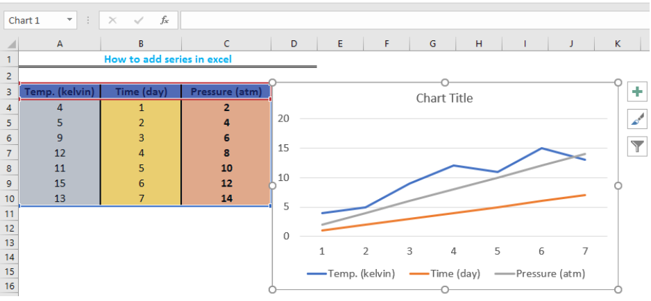 Figure 1: How to add data series in excel
How to Add Series in Excel
- To do this, we will tabulate our series of data and add the series name as title.
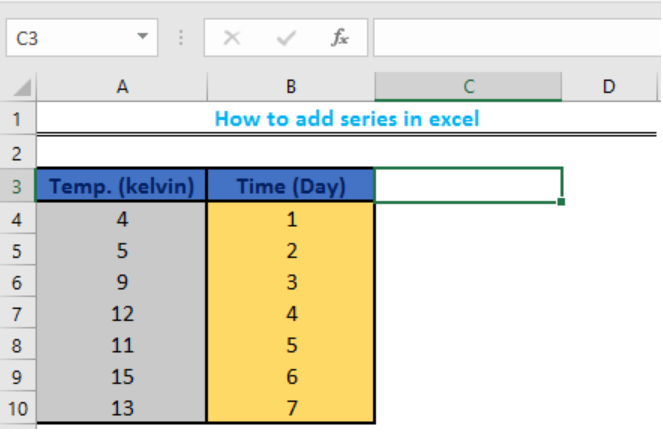 Figure 2: Data to create series in excel
- We will plot our chart with the data by clicking on insert and select a line chart
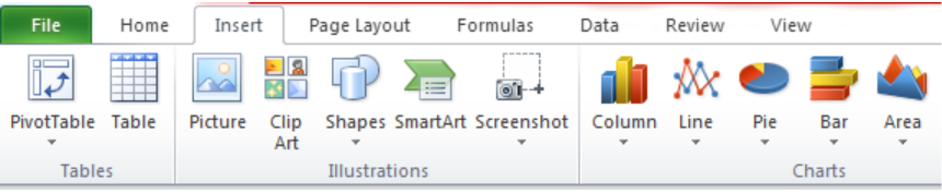 Figure 3: Click on Insert
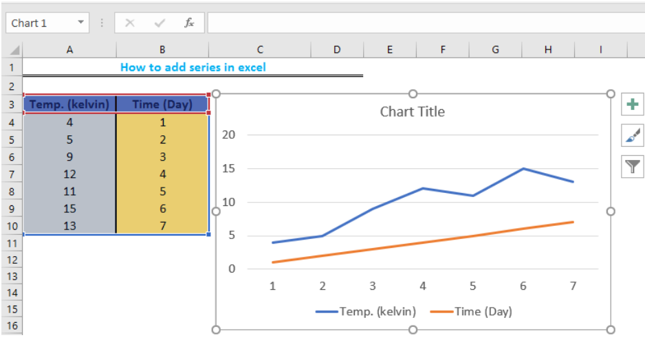 Figure 4: Line chart
- We will now create a column to add a new series of data
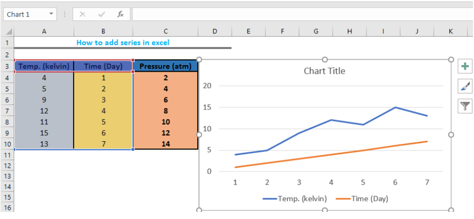 Figure 5: New set of data
When we click on the chart, it will highlight both the Temp. and Time columns, indicating the source of data. We will now drag the Fill handle (the box at the bottom-right when we click a cell) of the highlighted titles in Cells A3 and B3 over the new column created in Cell C3 to create the data series on the chart.
 Figure 6: New data series added to chart
- We can remove the data series from the chart by clicking on the line and pressing the delete key.
Instant Connection to an Expert through our Excelchat Service
Most of the time, the problem you will need to solve will be more complex than a simple application of a formula or function. If you want to save hours of research and frustration, try our live Excelchat service! Our Excel Experts are available 24/7 to answer any Excel question you may have. We guarantee a connection within 30 seconds and a customized solution within 20 minutes.
In this video, we’ll take a closer look at data series.
When you create a chart in Excel, you’re plotting numeric data organized into one or more «data series».
A data series is just a fancy name for a collection of related numbers in the same row, or the same column.
For example, this data shows yearly sales of shorts, sandals, t-shirts, and hoodies for an online surf shop.
If I create a column chart with the default options, we get a chart with three data series, one for each year.
In this chart, data series come from columns, and each column contains 4 values, one for each product.
Notice that Excel has used the column headers to name each data series, and that these names correspond to items you see listed in the legend.
You can verify and edit data series at any time by right-clicking and choosing Select Data.
In the Select Data Source window, data series are listed on the left. If I edit one of the entries, you can see that the data series has both a name and range of values.
You’re free to edit this information manually.
So what are the values listed on the right side of Select Data Source window?
These are axis labels, in this case, Horizontal axis labels, as you can see on the chart.
In short, this chart pulls data series names from columns, and axis labels from rows.
If I click the Switch Row/Column button, this is reversed.
The data series now come from rows and axis labels come from columns.
Again, notice the legend lists data series names.
Finally, I want to point out that when you select a data series, you’ll see formula in the formula bar. This formula is based on the SERIES function, which takes four arguments:
=SERIES([Series Name],[X Values],[Y Values],[Plot Order])
As I select each series, you can see these arguments change to match the data highlighted on the worksheet.
You can edit the SERIES formula if you like. For example, if I change plot order for the shorts data series to 4, Excel automatically plots the series last, and adjusts the order of the other series automatically.