
A pivot table in Excel is an extraction or resumé of your original table with source data. A pivot table can provide quick answers to questions about your table that can otherwise only be answered by complicated formulas.
Contents
- 1 What does pivoting mean in Excel?
- 2 What’s the point of a pivot table?
- 3 What is the difference between a table and a pivot table in Excel?
- 4 What is Vlookup in Excel?
- 5 What is pivot table example?
- 6 What is the difference between pivot table and Pivot Chart?
- 7 What is pivot table in simple words?
- 8 What are the 4 quadrants of a Pivot Table?
- 9 What is the difference between Pivot Table and Vlookup?
- 10 What is macro in Excel?
- 11 What is concatenate in Excel?
- 12 How is Xlookup different from VLOOKUP?
- 13 How do you create a pivot table step by step?
- 14 How do I edit a pivot table in Excel?
- 15 How do you read pivot points?
- 16 How many types of pivot tables are there?
- 17 What are slicers used for?
- 18 How do I create a pivot table in a spreadsheet?
- 19 How many columns can be in a PivotTable?
- 20 What is a quadrant chart?
What does pivoting mean in Excel?
A pivot table is a statistics tool that summarizes and reorganizes selected columns and rows of data in a spreadsheet or database table to obtain a desired report. The tool does not actually change the spreadsheet or database itself, it simply “pivots” or turns the data to view it from different perspectives.
What’s the point of a pivot table?
A PivotTable is an interactive way to quickly summarize large amounts of data. You can use a PivotTable to analyze numerical data in detail, and answer unanticipated questions about your data. A PivotTable is especially designed for: Querying large amounts of data in many user-friendly ways.
What is the difference between a table and a pivot table in Excel?
An Excel table is basically just a very simple database, consisting of one table. It has data elements (columns) and a set of members having those data elements (rows). It is detailed at the row level. A Pivot Table is a reporting and summation tool that gives you information *about* an Excel table.
What is Vlookup in Excel?
VLOOKUP stands for ‘Vertical Lookup’. It is a function that makes Excel search for a certain value in a column (the so called ‘table array’), in order to return a value from a different column in the same row.
What is pivot table example?
A Pivot table is a table of stats which summarizes the data as sums, averages, and many other statistical measures. Let’s assume that we got data of any real estate project with different fields like type of flats, block names, area of the individual flats, and their different cost as per different services, etc.
What is the difference between pivot table and Pivot Chart?
Pivot Tables allow you to create a powerful view with data summarized in a grid, both in horizontal and vertical columns (also known as Matrix Views or Cross Tabs).A Pivot Chart is an interactive graphical representation of the data in your Zoho Creator application.
What is pivot table in simple words?
A pivot table is a table of grouped values that aggregates the individual items of a more extensive table (such as from a database, spreadsheet, or business intelligence program) within one or more discrete categories.They arrange and rearrange (or “pivot”) statistics in order to draw attention to useful information.
What are the 4 quadrants of a Pivot Table?
The 4 Areas of a Pivot Table
- Introduction.
- Values area.
- Row area.
- Column area.
- Filter area.
What is the difference between Pivot Table and Vlookup?
A pivot table is a table of statistics that help to summarize and reorganize the data of a wide/broad table.On the other hand, VLOOKUP is a function which used in excel when you are required to find things/value in a data or range by row. In this article, we look at how to use VLookup within the Pivot Table.
If you have tasks in Microsoft Excel that you do repeatedly, you can record a macro to automate those tasks. A macro is an action or a set of actions that you can run as many times as you want. When you create a macro, you are recording your mouse clicks and keystrokes.
What is concatenate in Excel?
The word concatenate is just another way of saying “to combine” or “to join together”. The CONCATENATE function allows you to combine text from different cells into one cell. In our example, we can use it to combine the text in column A and column B to create a combined name in a new column.
How is Xlookup different from VLOOKUP?
XLOOKUP defaults to an exact match. VLOOKUP defaults to an “approximate” match, requiring that you add the “false” argument at the end of your VLOOKUP to perform an exact match.XLOOKUP can perform horizontal or vertical lookups. The XLOOKUP replaces both the VLOOKUP and HLOOKUP.
How do you create a pivot table step by step?
How to Create a Pivot Table
- Enter your data into a range of rows and columns.
- Sort your data by a specific attribute.
- Highlight your cells to create your pivot table.
- Drag and drop a field into the “Row Labels” area.
- Drag and drop a field into the “Values” area.
- Fine-tune your calculations.
How do I edit a pivot table in Excel?
Edit a pivot table. Click anywhere in a pivot table to open the editor. Add data—Depending on where you want to add data, under Rows, Columns, or Values, click Add. Change row or column names—Double-click a Row or Column name and enter a new name.
How do you read pivot points?
The first way is to determine the overall market trend. If the pivot point price is broken in an upward movement, then the market is bullish. If the price drops through the pivot point, then it’s is bearish. The second method is to use pivot point price levels to enter and exit the markets.
How many types of pivot tables are there?
Pivot Tables have three different layouts that you can choose from: Compact, Outline, and Tabular Form.
What are slicers used for?
Slicers provide buttons that you can click to filter tables, or PivotTables. In addition to quick filtering, slicers also indicate the current filtering state, which makes it easy to understand what exactly is currently displayed. You can use a slicer to filter data in a table or PivotTable with ease.
How do I create a pivot table in a spreadsheet?
Open a Google Sheets spreadsheet, and select all of the cells containing data. Click Data > Pivot Table. Check if Google’s suggested pivot table analyses answer your questions. To create a customized pivot table, click Add next to Rows and Columns to select the data you’d like to analyze.
How many columns can be in a PivotTable?
By default, the field list shows a list of the fields at the top, and the four pivot table areas in a square at the bottom. You can change that layout, by using a command on the field list.
What is a quadrant chart?
Quadrant charts are bubble charts with a background that is divided into four equal sections. Quadrant charts are useful for plotting data that contains three measures using an X-axis, a Y-axis, and a bubble size that represents the value of the third measure. You can also specify a default measure.
Last Update: Jan 03, 2023
This is a question our experts keep getting from time to time. Now, we have got the complete detailed explanation and answer for everyone, who is interested!
Asked by: Nicola Schuppe
Score: 5/5
(33 votes)
A pivot table is a table of grouped values that aggregates the individual items of a more extensive table within one or more discrete categories. This summary might include sums, averages, or other statistics, which the pivot table groups together using a chosen aggregation function applied to the grouped values.
What is a pivot table and what is it used for?
A PivotTable is an interactive way to quickly summarize large amounts of data. You can use a PivotTable to analyze numerical data in detail, and answer unanticipated questions about your data. A PivotTable is especially designed for: Querying large amounts of data in many user-friendly ways.
What is the use of pivot in Excel?
A pivot table in Excel is an extraction or resumé of your original table with source data. A pivot table can provide quick answers to questions about your table that can otherwise only be answered by complicated formulas.
What does pivoting mean in Excel?
A Pivot Table is used to summarise, sort, reorganise, group, count, total or average data stored in a table. It allows us to transform columns into rows and rows into columns. It allows grouping by any field (column), and using advanced calculations on them.
How do I do a pivot table in Excel?
To insert a pivot table, execute the following steps.
- Click any single cell inside the data set.
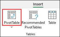
- On the Insert tab, in the Tables group, click PivotTable. The following dialog box appears. Excel automatically selects the data for you. The default location for a new pivot table is New Worksheet.
- Click OK.
37 related questions found
Why are pivot tables so important?
Pivot tables are important because they allow anyone to filter and extract significance about the data set they are working with. Pivot tables allow anyone to look at their data in a number of ways and perspectives.
How do you create a pivot table step by step?
How to Create a Pivot Table
- Enter your data into a range of rows and columns.
- Sort your data by a specific attribute.
- Highlight your cells to create your pivot table.
- Drag and drop a field into the «Row Labels» area.
- Drag and drop a field into the «Values» area.
- Fine-tune your calculations.
What is the difference between Pivot Table and Pivot Chart?
Pivot Tables allow you to create a powerful view with data summarized in a grid, both in horizontal and vertical columns (also known as Matrix Views or Cross Tabs). … A Pivot Chart is an interactive graphical representation of the data in your Zoho Creator application.
How can I learn Excel quickly?
5 Tips for Learning Excel
- Practice Simple Math Problems in Excel. When it comes to Excel, it’s easiest to start with basic math. …
- Learn How to Create Tables. …
- Learn How to Create Charts. …
- Take Excel Training Courses. …
- Earn a Microsoft Office Specialist Certification.
What does just pivot mean?
pivot Add to list Share. To pivot is to turn or rotate, like a hinge. Or a basketball player pivoting back and forth on one foot to protect the ball. When you’re not talking about a type of swiveling movement, you can use pivot to mean the one central thing that something depends upon.
What are the features of pivot table?
The seven unique features
- Totaling values.
- Hierarchical grouping by rows and columns.
- Persisting node states on dynamic updates.
- Displaying no data items.
- Conditionally formatting values with color and text styles.
- Linking with relevant page URLs.
- Interactive sorting by value columns.
Why is VLOOKUP used?
When you need to find information in a large spreadsheet, or you are always looking for the same kind of information, use the VLOOKUP function. VLOOKUP works a lot like a phone book, where you start with the piece of data you know, like someone’s name, in order to find out what you don’t know, like their phone number.
What is pivot table explain with example?
A pivot table is a statistics tool that summarizes and reorganizes selected columns and rows of data in a spreadsheet or database table to obtain a desired report. … This refers to a tool specific to Excel for creating pivot tables.
What is pivot strategy?
A pivot means fundamentally changing the direction of a business when you realize the current products or services aren’t meeting the needs of the market. The main goal of a pivot is to help a company improve revenue or survive in the market, but the way you pivot your business can make all the difference.
How do you use a pivot chart?
Select a cell in your PivotTable. On the Insert tab, select the Insert Chart dropdown menu, and then click any chart option. The chart will now appear in the worksheet.
…
Create a chart from a PivotTable
- Select a cell in your table.
- Select PivotTable Tools > Analyze > PivotChart .
- Select a chart.
- Select OK.
Can I learn Excel in a day?
It’s impossible to learn Excel in a day or a week, but if you set your mind to understanding individual processes one by one, you’ll soon find that you have a working knowledge of the software. Make your way through these techniques, and it won’t be long before you’re comfortable with the fundamentals of Excel.
What Excel skills are employers looking for?
What Are the Top Advanced Excel Skills for Administrative and Accounting Jobs?
- Data Simulations. There are many kinds of data simulations. …
- VLOOKUP and XLOOKUP. These functions allow you to find content in cells of the Excel table. …
- Advanced Conditional Formatting. Microsoft 365. …
- INDEX/MATCH. …
- Pivot Tables and Reporting. …
- Macros.
Can I learn Excel on my phone?
These Android applications for learning Excel are of a great use, however, all of them offer the standard way of reading and learning. keySkillset innovates the learning process and offers a Game that will help you learn Excel through shortcuts.
What are the different types of pivot table?
Pivot Tables have three different layouts that you can choose from: Compact, Outline, and Tabular Form.
How do you read pivot points?
The first way is to determine the overall market trend. If the pivot point price is broken in an upward movement, then the market is bullish. If the price drops through the pivot point, then it’s is bearish. The second method is to use pivot point price levels to enter and exit the markets.
Does access have pivot tables?
Create a PivotTable view. You can also create PivotTable and PivotChart views for Access queries, tables and forms.
What is the first step of creating pivot table?
Manually create a PivotTable
- Click a cell in the source data or table range.
- Go to Insert > PivotTable. …
- Excel will display the Create PivotTable dialog with your range or table name selected. …
- In the Choose where you want the PivotTable report to be placed section, select New Worksheet, or Existing Worksheet.
What is Vlookup function in Excel?
VLOOKUP stands for ‘Vertical Lookup’. It is a function that makes Excel search for a certain value in a column (the so called ‘table array’), in order to return a value from a different column in the same row.
What is a pivot table field name?
The pivot table error, «field name is not valid», usually appears because one or more of the heading cells in the source data is blank. To create a pivot table, you need a heading for each column. … If there are any merged cells in the heading row, unmerge them, and add a heading in each separate cell.
If you are reading this tutorial, there is a big chance you have heard of (or even used) the Excel Pivot Table. It’s one of the most powerful features in Excel (no kidding).
The best part about using a Pivot Table is that even if you don’t know anything in Excel, you can still do pretty awesome things with it with a very basic understanding of it.
Let’s get started.
Click here to download the sample data and follow along.
What is a Pivot Table and Why Should You Care?
A Pivot Table is a tool in Microsoft Excel that allows you to quickly summarize huge datasets (with a few clicks).
Even if you’re absolutely new to the world of Excel, you can easily use a Pivot Table. It’s as easy as dragging and dropping rows/columns headers to create reports.
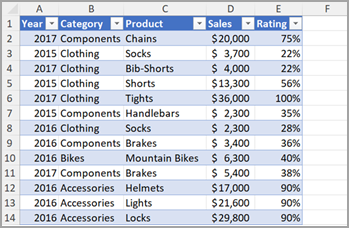
Suppose you have a dataset as shown below:
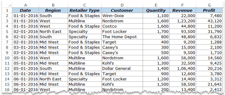
This is sales data that consists of ~1000 rows.
It has the sales data by region, retailer type, and customer.
Now your boss may want to know a few things from this data:
- What were the total sales in the South region in 2016?
- What are the top five retailers by sales?
- How did The Home Depot’s performance compare against other retailers in the South?
You can go ahead and use Excel functions to give you the answers to these questions, but what if suddenly your boss comes up with a list of five more questions.
You’ll have to go back to the data and create new formulas every time there is a change.
This is where Excel Pivot Tables comes in really handy.
Within seconds, a Pivot Table will answer all these questions (as you’ll learn below).
But the real benefit is that it can accommodate your finicky data-driven boss by answering his questions immediately.
It’s so simple, you may as well take a few minutes and show your boss how to do it himself.
Hopefully, now you have an idea of why Pivot Tables are so awesome. Let’s go ahead and create a Pivot Table using the data set (shown above).
Inserting a Pivot Table in Excel
Here are the steps to create a pivot table using the data shown above:
As soon as you click OK, a new worksheet is created with the Pivot Table in it.
While the Pivot Table has been created, you’d see no data in it. All you’d see is the Pivot Table name and a single line instruction on the left, and Pivot Table Fields on the right.
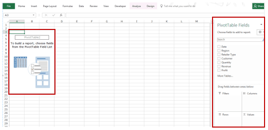
Now before we jump into analyzing data using this Pivot Table, let’s understand what are the nuts and bolts that make an Excel Pivot Table.
Also read: 10 Excel Pivot Table Keyboard Shortcuts
The Nuts & Bolts of an Excel Pivot Table
To use a Pivot Table efficiently, it’s important to know the components that create a pivot table.
In this section, you’ll learn about:
- Pivot Cache
- Values Area
- Rows Area
- Columns Area
- Filters Area
Pivot Cache
As soon as you create a Pivot Table using the data, something happens in the backend. Excel takes a snapshot of the data and stores it in its memory. This snapshot is called the Pivot Cache.
When you create different views using a Pivot Table, Excel does not go back to the data source, rather it uses the Pivot Cache to quickly analyze the data and give you the summary/results.
The reason a pivot cache gets generated is to optimize the pivot table functioning. Even when you have thousands of rows of data, a pivot table is super fast in summarizing the data. You can drag and drop items in the rows/columns/values/filters boxes and it will instantly update the results.
Note: One downside of pivot cache is that it increases the size of your workbook. Since it’s a replica of the source data, when you create a pivot table, a copy of that data gets stored in the Pivot Cache.
Read More: What is Pivot Cache and How to Best Use It.
Values Area
The Values Area is what holds the calculations/values.
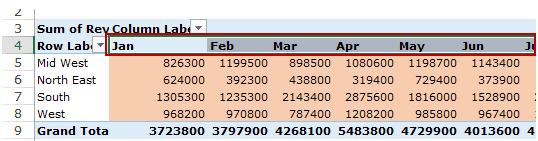
Based on the data set shown at the beginning of the tutorial, if you quickly want to calculate total sales by region in each month, you can get a pivot table as shown below (we’ll see how to create this later in the tutorial).
The area highlighted in orange is the Values Area.
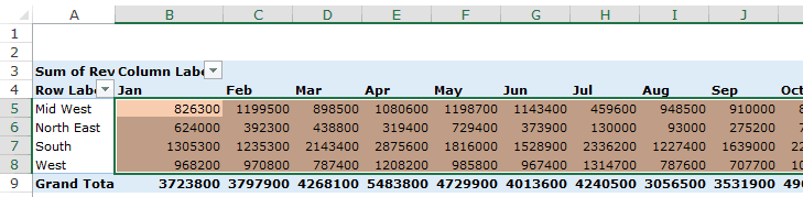
In this example, it has the total sales in each month for the four regions.
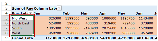
Rows Area
The headings to the left of the Values area makes the Rows area.
In the example below, the Rows area contains the regions (highlighted in red):
Columns Area
The headings at the top of the Values area makes the Columns area.
In the example below, Columns area contains the months (highlighted in red):
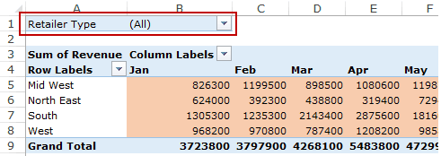
Filters Area
Filters area is an optional filter that you can use to further drill down in the data set.
For example, if you only want to see the sales for Multiline retailers, you can select that option from the drop down (highlighted in the image below), and the Pivot Table would update with the data for Multiline retailers only.
Analyzing Data Using the Pivot Table
Now, let’s try and answer the questions by using the Pivot Table we have created.
Click here to download the sample data and follow along.
To analyze data using a Pivot Table, you need to decide how you want the data summary to look in the final result. For example, you may want all the regions in the left and the total sales right next to it. Once you have this clarity in mind, you can simply drag and drop the relevant fields in the Pivot Table.
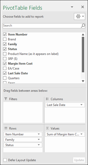
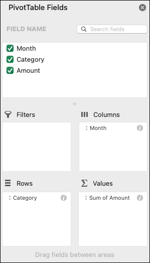
In the Pivot Tabe Fields section, you have the fields and the areas (as highlighted below):
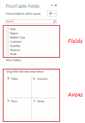
The Fields are created based on the backend data used for the Pivot Table. The Areas section is where you place the fields, and according to where a field goes, your data is updated in the Pivot Table.
It’s a simple drag and drop mechanism, where you can simply drag a field and put it in one of the four areas. As soon as you do this, it will appear in the Pivot Table in the worksheet.
Now let’s try and answer the questions your manager had using this Pivot Table.
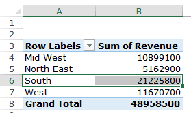
Q1: What were the total sales in the South region?
Drag the Region field in the Rows area and the Revenue field in the Values area. It would automatically update the Pivot Table in the worksheet.
Note that as soon as you drop the Revenue field in the Values area, it becomes Sum of Revenue. By default, Excel sums all the values for a given region and shows the total. If you want, you can change this to Count, Average, or other statistics metrics. In this case, the sum is what we needed.
The answer to this question would be 21225800.
Q2 What are the top five retailers by sales?
Drag the Customer field in the Row area and Revenue field in the values area. In case, there are any other fields in the area section and you want to remove it, simply select it and drag it out of it.
You’ll get a Pivot Table as shown below:
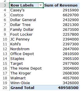
Note that by default, the items (in this case the customers) are sorted in an alphabetical order.
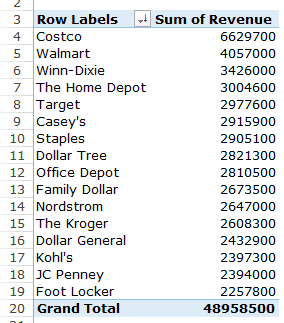
To get the top five retailers, you can simply sort this list and use the top five customer names. To do this:
This will give you a sorted list based on total sales.
Q3: How did The Home Depot’s performance compare against other retailers in the South?
You can do a lot of analysis for this question, but here let’s just try and compare the sales.
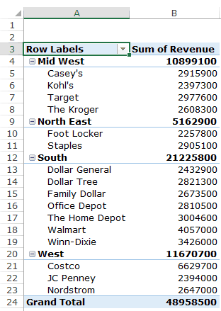
Drag the Region Field in the Rows area. Now drag the Customer field in the Rows area below the Region field. When you do this, Excel would understand that you want to categorize your data first by region and then by customers within the regions. You’ll have something as shown below:
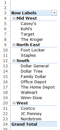
Now drag the Revenue field in the Values area and you’ll have the sales for each customer (as well as the overall region).
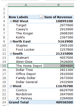
You can sort the retailers based on the sales figures by following the below steps:
- Right-click on a cell that has the sales value for any retailer.
- Go to Sort –> Sort Largest to Smallest.
This would instantly sort all the retailers by the sales value.
Now you can quickly scan through the South region and identify that The Home Depot sales were 3004600 and it did better than four retailers in the South region.
Now there are more than one ways to skin the cat. You can also put the Region in the Filter area and then only select the South Region.
Click here to download the sample data.
I hope this tutorial gives you a basic overview of Excel Pivot Tables and helps you in getting started with it.
Here are some more Pivot Table Tutorials you may like:
- Preparing Source Data For Pivot Table.
- How to Apply Conditional Formatting in a Pivot Table in Excel.
- How to Group Dates in Pivot Tables in Excel.
- How to Group Numbers in Pivot Table in Excel.
- How to Filter Data in a Pivot Table in Excel.
- Using Slicers in Excel Pivot Table.
- How to Replace Blank Cells with Zeros in Excel Pivot Tables.
- How to Add and Use an Excel Pivot Table Calculated Fields.
- How to Refresh Pivot Table in Excel.
Table of contents
- Introduction to Pivot tables in excel
- What is a Pivot table in excel?
- How to Create a Pivot Table?
- Here is the Step By Step Guide to creating a pivot table
- Examples of Pivot tables
- What are pivot tables used for?
- Benefits of using Pivot Table
- Pivot Tables are simple to use.
- Pivot tables can generate real-time data.
- The Pivot Table facilitates data analysis.
- A pivot table simplifies data summarization.
- A pivot table can help you find data patterns.
- Pivot tables can assist in making faster decisions.
- Difference between Pivot table and Straight Table
- How to refresh Pivot Table?
- Free courses on Excel
- Conclusion
- Introduction to Pivot tables in excel
- What is a Pivot table in excel?
- How to Create a Pivot Table?
- Examples of Pivot tables
- What are pivot tables used for?
- Benefits of using Pivot Table
- Difference between Pivot table and Straight Table
- How to refresh Pivot Table?
- Free courses on Excel
Introduction to Pivot tables in excel
In today’s article, we will learn about the most important feature of Excel, i.e., How to Create a pivot table in excel and how to refresh the pivot table.
Our objective is to aid you with the most basic introduction and explanation of what a Pivot Table is that you can find. You will recognize the principles of pivot tables after reading this article.
You’ll understand how things work behind the scenes. You will also be upskilled in how to analyze business data.
This article is for you if you have never created a pivot table or if you have, but it feels like magic to you.
Let us first learn about what is a pivot table in excel?
What is a Pivot table in excel?
A pivot table is an essential data analysis tool. Many important business questions can be quickly answered using pivot tables. One of the reasons we create Pivot Tables is to pass data. We want to back up our story with data that are easy to understand and see. Although Pivot Tables are only tables and lack authentic visuals, they can still be used for Visual Storytelling.
A PivotTable is a powerful tool for calculating, summarizing, and analyzing data that allows you to see comparisons, patterns, and trends. PivotTables behave differently depending on the platform on which you run Excel.
A Pivot Table can be used to summarise, analyze, explore, and present summary data. PivotCharts add visualizations to the summary data in a PivotTable, allowing you to see comparisons, patterns, and trends effortlessly. PivotTables and PivotCharts both allow you to make informed decisions about critical data in your organization.
You can also create PivotTables by connecting to external data sources such as the SQL- Server tables, SQL- Server Analysis Services cubes, Azure Marketplace, Office Data Connection (.odc) files, XML files, Access databases, and text files, or by using existing PivotTables.
Mastering pivot tables may appear to be complicated. However, with a few basic principles, you can grasp them quickly. You will quickly catch up to your more advanced colleagues in this area. And, of course, you will increase your value on the job market.
So far, we’ve been speaking in broad strokes, with no specific tool. You can apply your new skills in any tool your company uses, including Microsoft Office, Libre Office, Open Office, Google Sheets, and many others. Let’s look at how the Pivot Table settings appear in the most popular tools so you’re familiar with them and ready to use them immediately!
To create a Pivot Table in most tools, highlight the sheet region and click a function (usually in the Data menu). Consider using Microsoft Office as an example.
There is a function in Microsoft Office named Ideas that can even suggest some basic Pivot Tables based on what is constructed on the current sheet. This can be an excellent point to start.
How to Create a Pivot Table?
Here is the Step By Step Guide to creating a pivot table
- Step1: In Excel for Windows, make a PivotTable.
- Choose the cells from which you want to create a PivotTable
- Go to Insert Option and click on Pivot Table
- Select the location for the PivotTable report.
- At last, click on the OK option.
- Step2: Creating Pivot Table from different sources.
- Step3: Create your own Pivot Table by using the given data.
- To add a field to your PivotTable, check the box next to the field name in the PivotTables Fields pane.
- Drag the field to the target area to move it from one area to another.
In Excel for Windows, make a PivotTable.
- Choose the cells from which you want to create a PivotTable. Please keep in mind that your data should be organised in columns with a single header row.
- Go to Insert Option and click on Pivot Table.

- Based on an existing table or range, this will generate a PivotTable.

- Take note: Choosing and adding the given data to the Data Model will insert the table or range used for this PivotTable into the workbook’s data model.
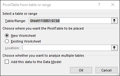
- Select the location for the PivotTable report. Choose New Worksheet to insert the PivotTable into a new worksheet or Existing Worksheet and specify where you want the PivotTable to appear.
- At last, click on the OK option.
Creating Pivot Table from different sources
- You can choose from other possible sources for your PivotTable by clicking the down arrow on the button.
- In addition, to make use of an existing table or range, you have three other options for populating your Pivot Table.
- Note: Depending on your organization’s IT settings, your organization’s name may appear on the button. “From Power BI (Microsoft),” for example.

Creating your own Pivot Table by using given data
To add a field to your PivotTable, check the box next to the field name in the PivotTables Fields pane.
Note that selected fields are added to their default areas: non-numeric fields to Rows, date and time hierarchies to Columns, and numeric fields to Values.

Drag the field to the target area to move it from one area to another.
Examples of Pivot tables
Let us look at some examples where we can use the Pivot table.
Create a list of unique values using a pivot table. Because pivot tables summarise data, they can be used to locate distinct values within a table column. This is a quick way to see all the values in a field and find typos and other inconsistencies.
A pivot table can do things like
- group items/records/rows into categories
- count the number of items in each category
- sum the item values or compute the average
- find the minimal or maximal value, and so on.
We’ll see how pivot tables work in a few simple steps. Then, creating pivot tables will no longer be difficult.
What are pivot tables used for?
The following vital point to remember about pivot tables is why we use them.
A Pivot Table is a user-friendly tool for quickly summarizing a big size of data. A PivotTable can be used to analyze numerical data in-depth and answer random questions about your data. A PivotTable is beneficial for:
- If you have a large size, data can be queried in a variety of user-friendly ways.
- Numeric data subtotaling and aggregation, data summarization by categories and subcategories, and custom calculations and formulas.
- Expanding and collapsing data levels to focus your results, as well as drilling down to details from summary data for areas of interest to you.
- If you want to see different summaries of the source data, move rows to columns or columns to rows (or “pivot”).
- Various features include filtering, sorting, grouping, and conditionally formatting. The most valuable and exciting subset of data allows you to concentrate on only the information you need.
- Concise, attractive, and annotated reports can be presented online or in print.
For example, on the left is a simple list of household expenses, and on the right is a PivotTable based on the list:

Benefits of using Pivot Table
Here are quite a few of the advantages and benefits of using Pivot Tables:
Pivot Tables are simple to use.
One significant advantage of pivot tables is their ease of use. Everyone can find it simple to summarise collected data. It’s as simple as dragging the columns to different table sections. The columns can also be rearranged and moved as desired by any user with the click of a button.
Pivot tables can generate real-time data.
Another essential feature of a pivot table is its ability to generate data in real-time. Whether a user enters equations directly into the pivot table or relies on formulas, this instrument can generate instant or immediate data. And using this tool, a user can quickly compare the information. It is as simple as creating columns on tables and dragging and dropping desired information to compare. This is especially useful if a pivot table user is short on time.
The Pivot Table facilitates data analysis.
Data analysis is much easier with pivot tables. Users will benefit from its use by being able to handle large amounts of data and analyze them more quickly. Pivot tables permit you to take a large data size and work with it so that you only need to see a small number of data fields. This will significantly facilitate the analysis of large amounts of data. Furthermore, pivot tables enhance the data analysis experience. It is now more interactive. The tables allow the user to easily drag and drop data, making the data table interactive. This is a critical tool for quick and efficient work with Microsoft Excel.
A pivot table simplifies data summarization.
Pivot tables can be extremely useful for quickly and easily summarising data. It will help any user create a summary from a large amount of disorganized data in the form of rows and columns. This tool allows you to condense large amounts of information into smaller amounts. Furthermore, the data can be summarised in a straightforward format that anyone can understand. With this tool, users can label and sort rows and columns in any way they want, and data can be arranged according to their needs and how they want it to be presented. Most importantly, pivot tables make it easier to segment data analytics collected in a spreadsheet or database.
A pivot table can help you find data patterns.
Forecasting is critical in any management, whether in business or in any organization. Excel pivot tables can help any user create customized tables from large data groups in this task. And manipulating data in this manner will aid in the discovery of recurring patterns in the data. This, in turn, will aid in accurate data forecasting. A pivot table generates accurate reports more quickly. Another essential feature of pivot tables is that they can assist any user in efficiently and reliably creating or formulating reports and demonstrations. It will fend off any user from manually creating reports. That means more time for other tasks and activities. Furthermore, a pivot table user can include links to external sources, if any, in their report, making reports and presentations more efficient and convincing. A pivot table is one of the few tools available to users for gaining a deeper understanding of analytics data. This tool can generate multiple reports from the same collected data contained in a single file.
It would keep you away from ‘cut and paste’ and require you to take more steps to get to the data that a user needs. Remember that in today’s world, information is currency, and the faster you can acquire it, the better.
Pivot tables can assist in making faster decisions.
With the modern world’s fast-paced demand, quick decision-making is critical. This is incredibly accurate for business owners and executives. A pivot table can be a valuable tool in this regard. It saves a significant amount of time. It is a very valuable reporting tool because it allows users to analyze data and make decisions without much difficulty quickly. This is exceptionally useful in the business world, where making precise and timely decisions in a short period is critical.
Difference between Pivot table and Straight Table
The distinction between a straight table and a pivot table
Table Pivot
The pivot table displays dimensions and expressions as tables. There is no formal restriction on the number of dimensions or expressions that can be used. A pivot table can be defined without using expressions, resulting in a tree view for navigating the dimension levels.
Straight table
The straight table differs from the pivot table in that it does not support subtotals, and the dimension grouping is displayed in record form, with each row of the table containing field and expression values.
How to refresh Pivot Table?
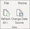
- When you add new data to a PivotTable data source, all PivotTables built on that data source must be refreshed.
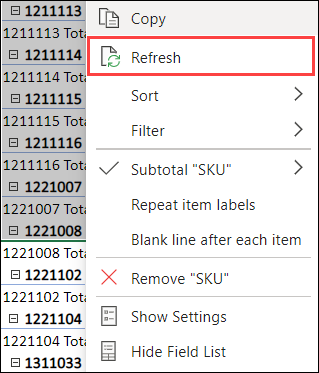
- To refresh only one PivotTable, right-click anywhere in the PivotTable range and choose Refresh.
- If you have multiple PivotTables, first select any cell in any PivotTable, then go to PivotTable Analyze on the Ribbon > click the arrow under the Refresh button and select Refresh All.

Free courses on Excel
- Excel for beginners
- Excel Tips and Tricks
- Excel Regression Analysis
- VLOOKUP in Excel
- Data Analytics using Excel
- Conditional Formatting in Excel
Conclusion
A pivot table in excel is not, as some may believe, cheating or a false or incorrect method of data management. It is a fantastic tool for faster, easier, and more reliable data collection, analysis, sorting, summarising, report and presentation creation, and assisting any user in making more reliable decisions. This is how we can create interactive reports in Excel using the Pivot table feature. A pivot table is an excellent tool if you enjoy experimenting with data sets. Just keep exploring the distinct features of the Pivot table to get a good understanding. Learn more such Excel tips and tricks today with us!
A PivotTable is a powerful tool to calculate, summarize, and analyze data that lets you see comparisons, patterns, and trends in your data. PivotTables work a little bit differently depending on what platform you are using to run Excel.


-
Select the cells you want to create a PivotTable from.
Note: Your data should be organized in columns with a single header row. See the Data format tips and tricks section for more details.
-
Select Insert > PivotTable.

-
This will create a PivotTable based on an existing table or range.
Note: Selecting Add this data to the Data Model will add the table or range being used for this PivotTable into the workbook’s Data Model. Learn more.
-
Choose where you want the PivotTable report to be placed. Select New Worksheet to place the PivotTable in a new worksheet or Existing Worksheet and select where you want the new PivotTable to appear.
-
Click OK.
By clicking the down arrow on the button, you can select from other possible sources for your PivotTable. In addition to using an existing table or range, there are three other sources you can select from to populate your PivotTable.
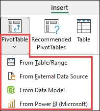
Note: Depending on your organization’s IT settings you might see your organization’s name included in the button. For example, «From Power BI (Microsoft)»
Get from External Data Source
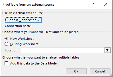
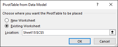
Get from Data Model
Use this option if your workbook contains a Data Model, and you want to create a PivotTable from multiple Tables, enhance the PivotTable with custom measures, or are working with very large datasets.
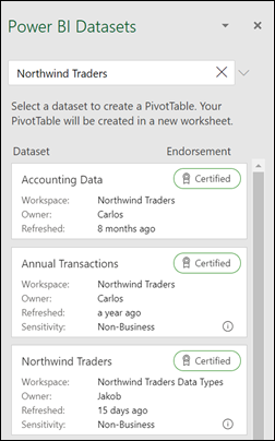
Get from Power BI
Use this option if your organization uses Power BI and you want to discover and connect to endorsed cloud datasets you have access to.
-
To add a field to your PivotTable, select the field name checkbox in the PivotTables Fields pane.
Note: Selected fields are added to their default areas: non-numeric fields are added to Rows, date and time hierarchies are added to Columns, and numeric fields are added to Values.
-
To move a field from one area to another, drag the field to the target area.
If you add new data to your PivotTable data source, any PivotTables that were built on that data source need to be refreshed. To refresh just one PivotTable you can right-click anywhere in the PivotTable range, then select Refresh. If you have multiple PivotTables, first select any cell in any PivotTable, then on the Ribbon go to PivotTable Analyze > click the arrow under the Refresh button and select Refresh All.
Summarize Values By
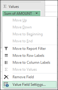
By default, PivotTable fields that are placed in the Values area will be displayed as a SUM. If Excel interprets your data as text, it will be displayed as a COUNT. This is why it’s so important to make sure you don’t mix data types for value fields. You can change the default calculation by first clicking on the arrow to the right of the field name, then select the Value Field Settings option.
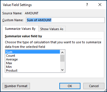
Next, change the calculation in the Summarize Values By section. Note that when you change the calculation method, Excel will automatically append it in the Custom Name section, like «Sum of FieldName», but you can change it. If you click the Number Format button, you can change the number format for the entire field.
Tip: Since the changing the calculation in the Summarize Values By section will change the PivotTable field name, it’s best not to rename your PivotTable fields until you’re done setting up your PivotTable. One trick is to use Find & Replace (Ctrl+H) >Find what > «Sum of«, then Replace with > leave blank to replace everything at once instead of manually retyping.
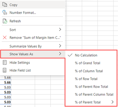
Show Values As
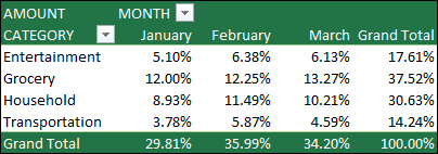
Instead of using a calculation to summarize the data, you can also display it as a percentage of a field. In the following example, we changed our household expense amounts to display as a % of Grand Total instead of the sum of the values.
Once you’ve opened the Value Field Setting dialog, you can make your selections from the Show Values As tab.
Display a value as both a calculation and percentage.
Simply drag the item into the Values section twice, then set the Summarize Values By and Show Values As options for each one.
-
Select a table or range of data in your sheet and select Insert > PivotTable to open the Insert PivotTable pane.
-
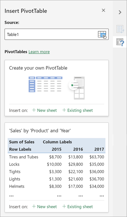
You can either manually create your own PivotTable or choose a recommended PivotTable to be created for you. Do one of the following:
-
On the Create your own PivotTable card, select either New sheet or Existing sheet to choose the destination of the PivotTable.
-
On a recommended PivotTable, select either New sheet or Existing sheet to choose the destination of the PivotTable.
Note: Recommended PivotTables are only available to Microsoft 365 subscribers.
You can change the data sourcefor the PivotTable data as you are creating it.
-
In the Insert PivotTable pane, select the text box under Source. While changing the Source, cards in the pane won’t be available.
-
Make a selection of data on the grid or enter a range in the text box.
-
Press Enter on your keyboard or the button to confirm your selection. The pane will update with new recommended PivotTables based on the new source of data.

Get from Power BI
Use this option if your organization uses Power BI and you want to discover and connect to endorsed cloud datasets you have access to.
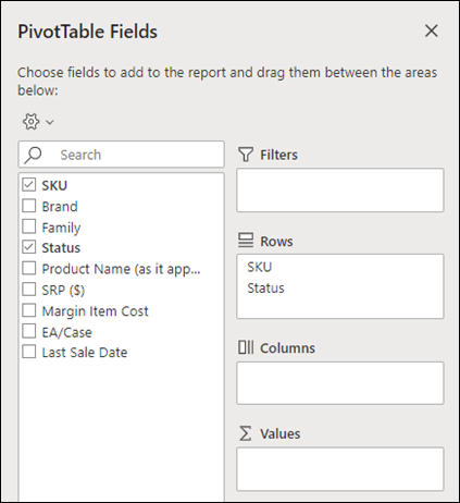
In the PivotTable Fields pane, select the check box for any field you want to add to your PivotTable.
By default, non-numeric fields are added to the Rows area, date and time fields are added to the Columns area, and numeric fields are added to the Values area.
You can also manually drag-and-drop any available item into any of the PivotTable fields, or if you no longer want an item in your PivotTable, drag it out from the list or uncheck it.
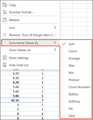
Summarize Values By
By default, PivotTable fields in the Values area will be displayed as a SUM. If Excel interprets your data as text, it will be displayed as a COUNT. This is why it’s so important to make sure you don’t mix data types for value fields.
Change the default calculation by right clicking on any value in the row and selecting the Summarize Values By option.
Show Values As
Instead of using a calculation to summarize the data, you can also display it as a percentage of a field. In the following example, we changed our household expense amounts to display as a % of Grand Total instead of the sum of the values.
Right click on any value in the column you’d like to show the value for. Select Show Values As in the menu. A list of available values will display.
Make your selection from the list.
To show as a % of Parent Total, hover over that item in the list and select the parent field you want to use as the basis of the calculation.
If you add new data to your PivotTable data source, any PivotTables built on that data source will need to be refreshed. Right-click anywhere in the PivotTable range, then select Refresh.
If you created a PivotTable and decide you no longer want it, select the entire PivotTable range and press Delete. It won’t have any effect on other data or PivotTables or charts around it. If your PivotTable is on a separate sheet which has no other data you want to keep, deleting the sheet is a fast way to remove the PivotTable.
-
Your data should be organized in a tabular format, and not have any blank rows or columns. Ideally, you can use an Excel table like in our example above.
-
Tables are a great PivotTable data source, because rows added to a table are automatically included in the PivotTable when you refresh the data, and any new columns will be included in the PivotTable Fields List. Otherwise, you need to either Change the source data for a PivotTable, or use a dynamic named range formula.
-
Data types in columns should be the same. For example, you shouldn’t mix dates and text in the same column.
-
PivotTables work on a snapshot of your data, called the cache, so your actual data doesn’t get altered in any way.
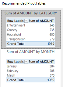
If you have limited experience with PivotTables, or are not sure how to get started, a Recommended PivotTable is a good choice. When you use this feature, Excel determines a meaningful layout by matching the data with the most suitable areas in the PivotTable. This helps give you a starting point for additional experimentation. After a recommended PivotTable is created, you can explore different orientations and rearrange fields to achieve your specific results. You can also download our interactive Make your first PivotTable tutorial.
-
Click a cell in the source data or table range.
-
Go to Insert > Recommended PivotTable.
-
Excel analyzes your data and presents you with several options, like in this example using the household expense data.
-
Select the PivotTable that looks best to you and press OK. Excel will create a PivotTable on a new sheet, and display the PivotTable Fields List

-
Click a cell in the source data or table range.
-
Go to Insert > PivotTable.
-
Excel will display the Create PivotTable dialog with your range or table name selected. In this case, we’re using a table called «tbl_HouseholdExpenses».
-
In the Choose where you want the PivotTable report to be placed section, select New Worksheet, or Existing Worksheet. For Existing Worksheet, select the cell where you want the PivotTable placed.
-
Click OK, and Excel will create a blank PivotTable, and display the PivotTable Fields list.
PivotTable Fields list
In the Field Name area at the top, select the check box for any field you want to add to your PivotTable. By default, non-numeric fields are added to the Row area, date and time fields are added to the Column area, and numeric fields are added to the Values area. You can also manually drag-and-drop any available item into any of the PivotTable fields, or if you no longer want an item in your PivotTable, simply drag it out of the Fields list or uncheck it. Being able to rearrange Field items is one of the PivotTable features that makes it so easy to quickly change its appearance.
PivotTable Fields list
-
Summarize by
By default, PivotTable fields that are placed in the Values area will be displayed as a SUM. If Excel interprets your data as text, it will be displayed as a COUNT. This is why it’s so important to make sure you don’t mix data types for value fields. You can change the default calculation by first clicking on the arrow to the right of the field name, then select the Field Settings option.
Next, change the calculation in the Summarize by section. Note that when you change the calculation method, Excel will automatically append it in the Custom Name section, like «Sum of FieldName», but you can change it. If you click the Number… button, you can change the number format for the entire field.
Tip: Since the changing the calculation in the Summarize by section will change the PivotTable field name, it’s best not to rename your PivotTable fields until you’re done setting up your PivotTable. One trick is to click Replace (on the Edit menu) >Find what > «Sum of«, then Replace with > leave blank to replace everything at once instead of manually retyping.
-
Show data as
Instead of using a calculation to summarize the data, you can also display it as a percentage of a field. In the following example, we changed our household expense amounts to display as a % of Grand Total instead of the sum of the values.
Once you’ve opened the Field Settings dialog, you can make your selections from the Show data as tab.
-
Display a value as both a calculation and percentage.
Simply drag the item into the Values section twice, right-click the value and select Field Settings, then set the Summarize by and Show data as options for each one.
If you add new data to your PivotTable data source, any PivotTables that were built on that data source need to be refreshed. To refresh just one PivotTable you can right-click anywhere in the PivotTable range, then select Refresh. If you have multiple PivotTables, first select any cell in any PivotTable, then on the Ribbon go to PivotTable Analyze > click the arrow under the Refresh button and select Refresh All.
If you created a PivotTable and decide you no longer want it, you can simply select the entire PivotTable range, then press Delete. It won’t have any affect on other data or PivotTables or charts around it. If your PivotTable is on a separate sheet that has no other data you want to keep, deleting that sheet is a fast way to remove the PivotTable.
Data format tips and tricks
-
Use clean, tabular data for best results.
-
Organize your data in columns, not rows.
-
Make sure all columns have headers, with a single row of unique, non-blank labels for each column. Avoid double rows of headers or merged cells.
-
Format your data as an Excel table (select anywhere in your data and then select Insert > Table from the ribbon).
-
If you have complicated or nested data, use Power Query to transform it (for example, to unpivot your data) so it is organized in columns with a single header row.
Need more help?
You can always ask an expert in the Excel Tech Community or get support in the Answers community.
PivotTable Recommendations are a part of the connected experience in Microsoft 365, and analyzes your data with artificial intelligence services. If you choose to opt out of the connected experience in Microsoft 365, your data will not be sent to the artificial intelligence service, and you will not be able to use PivotTable Recommendations. Read the Microsoft privacy statement for more details.
Related articles
Create a PivotChart
Use slicers to filter PivotTable data
Create a PivotTable timeline to filter dates
Create a PivotTable with the Data Model to analyze data in multiple tables
Create a PivotTable connected to Power BI Datasets
Use the Field List to arrange fields in a PivotTable
Change the source data for a PivotTable
Calculate values in a PivotTable
Delete a PivotTable