
Excel for Microsoft 365 Excel for Microsoft 365 for Mac Excel for the web Excel 2021 Excel 2019 Excel 2016 Excel 2013 Excel 2010 Excel 2007 More…Less
You can use a PivotTable to summarize, analyze, explore, and present summary data. PivotCharts complement PivotTables by adding visualizations to the summary data in a PivotTable, and allow you to easily see comparisons, patterns, and trends. Both PivotTables and PivotCharts enable you to make informed decisions about critical data in your enterprise. You can also connect to external data sources such as SQL Server tables, SQL Server Analysis Services cubes, Azure Marketplace, Office Data Connection (.odc) files, XML files, Access databases, and text files to create PivotTables, or use existing PivotTables to create new tables.
A PivotTable is an interactive way to quickly summarize large amounts of data. You can use a PivotTable to analyze numerical data in detail, and answer unanticipated questions about your data. A PivotTable is especially designed for:
-
Querying large amounts of data in many user-friendly ways.
-
Subtotaling and aggregating numeric data, summarizing data by categories and subcategories, and creating custom calculations and formulas.
-
Expanding and collapsing levels of data to focus your results, and drilling down to details from the summary data for areas of interest to you.
-
Moving rows to columns or columns to rows (or «pivoting») to see different summaries of the source data.
-
Filtering, sorting, grouping, and conditionally formatting the most useful and interesting subset of data enabling you to focus on just the information you want.
-
Presenting concise, attractive, and annotated online or printed reports.
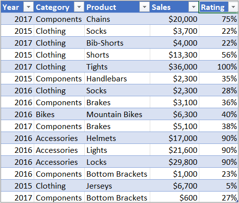
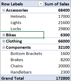
For example, here’s a simple list of household expenses on the left, and a PivotTable based on the list to the right:
|
Sales data |
Corresponding PivotTable |
|
|
|
For more information, see Create a PivotTable to analyze worksheet data.
After you create a PivotTable by selecting its data source, arranging fields in the PivotTable Field List, and choosing an initial layout, you can perform the following tasks as you work with a PivotTable:
Explore the data by doing the following:
-
Expand and collapse data, and show the underlying details that pertain to the values.
-
Sort, filter, and group fields and items.
-
Change summary functions, and add custom calculations and formulas.
Change the form layout and field arrangement by doing the following:
-
Change the PivotTable form: Compact, Outline, or Tabular.
-
Add, rearrange, and remove fields.
-
Change the order of fields or items.
Change the layout of columns, rows, and subtotals by doing the following:
-
Turn column and row field headers on or off, or display or hide blank lines.
-
Display subtotals above or below their rows.
-
Adjust column widths on refresh.
-
Move a column field to the row area or a row field to the column area.
-
Merge or unmerge cells for outer row and column items.
Change the display of blanks and errors by doing the following:
-
Change how errors and empty cells are displayed.
-
Change how items and labels without data are shown.
-
Display or hide blank rows
Change the format by doing the following:
-
Manually and conditionally format cells and ranges.
-
Change the overall PivotTable format style.
-
Change the number format for fields.
-
Include OLAP Server formatting.
For more information, see Design the layout and format of a PivotTable.
PivotCharts provide graphical representations of the data in their associated PivotTables. PivotCharts are also interactive. When you create a PivotChart, the PivotChart Filter Pane appears. You can use this filter pane to sort and filter the PivotChart’s underlying data. Changes that you make to the layout and data in an associated PivotTable are immediately reflected in the layout and data in the PivotChart and vice versa.
PivotCharts display data series, categories, data markers, and axes just as standard charts do. You can also change the chart type and other options such as the titles, the legend placement, the data labels, the chart location, and so on.
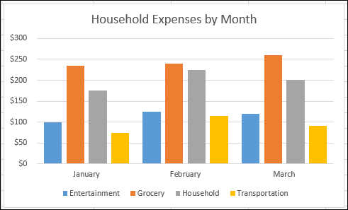
Here’s a PivotChart based on the PivotTable example above.
For more information, see Create a PivotChart.
If you are familiar with standard charts, you will find that most operations are the same in PivotCharts. However, there are some differences:
Row/Column orientation Unlike a standard chart, you cannot switch the row/column orientation of a PivotChart by using the Select Data Source dialog box. Instead, you can pivot the Row and Column labels of the associated PivotTable to achieve the same effect.
Chart types You can change a PivotChart to any chart type except an xy (scatter), stock, or bubble chart.
Source data Standard charts are linked directly to worksheet cells, while PivotCharts are based on their associated PivotTable’s data source. Unlike a standard chart, you cannot change the chart data range in a PivotChart’s Select Data Source dialog box.
Formatting Most formatting—including chart elements that you add, layout, and style—is preserved when you refresh a PivotChart. However, trendlines, data labels, error bars, and other changes to data sets are not preserved. Standard charts do not lose this formatting once it is applied.
Although you cannot directly resize the data labels in a PivotChart, you can increase the text font size to effectively resize the labels.
You can use data from a Excel worksheet as the basis for a PivotTable or PivotChart. The data should be in list format, with column labels in the first row, which Excel will use for Field Names. Each cell in subsequent rows should contain data appropriate to its column heading, and you shouldn’t mix data types in the same column. For instance, you shouldn’t mix currency values and dates in the same column. Additionally, there shouldn’t be any blank rows or columns within the data range.
Excel tables Excel tables are already in list format and are good candidates for PivotTable source data. When you refresh the PivotTable, new and updated data from the Excel table is automatically included in the refresh operation.
Using a dynamic named range To make a PivotTable easier to update, you can create a dynamic named range, and use that name as the PivotTable’s data source. If the named range expands to include more data, refreshing the PivotTable will include the new data.
Including totals Excel automatically creates subtotals and grand totals in a PivotTable. If the source data contains automatic subtotals and grand totals that you created by using the Subtotals command in the Outline group on the Data tab, use that same command to remove the subtotals and grand totals before you create the PivotTable.
You can retrieve data from an external data source such as a database, an Online Analytical Processing (OLAP) cube, or a text file. For example, you might maintain a database of sales records you want to summarize and analyze.
Office Data Connection files If you use an Office Data Connection (ODC) file (.odc) to retrieve external data for a PivotTable, you can input the data directly into a PivotTable. We recommend that you retrieve external data for your reports by using ODC files.
OLAP source data When you retrieve source data from an OLAP database or a cube file, the data is returned to Excel only as a PivotTable or a PivotTable that has been converted to worksheet functions. For more information, see Convert PivotTable cells to worksheet formulas.
Non-OLAP source data This is the underlying data for a PivotTable or a PivotChart that comes from a source other than an OLAP database. For example, data from relational databases or text files.
For more information, see Create a PivotTable with an external data source.
The PivotTable cache Each time that you create a new PivotTable or PivotChart, Excel stores a copy of the data for the report in memory, and saves this storage area as part of the workbook file — this is called the PivotTable cache. Each new PivotTable requires additional memory and disk space. However, when you use an existing PivotTable as the source for a new one in the same workbook, both share the same cache. Because you reuse the cache, the workbook size is reduced and less data is kept in memory.
Location requirements To use one PivotTable as the source for another, both must be in the same workbook. If the source PivotTable is in a different workbook, copy the source to the workbook location where you want the new one to appear. PivotTables and PivotCharts in different workbooks are separate, each with its own copy of the data in memory and in the workbooks.
Changes affect both PivotTables When you refresh the data in the new PivotTable, Excel also updates the data in the source PivotTable, and vice versa. When you group or ungroup items, or create calculated fields or calculated items in one, both are affected. If you need to have a PivotTable that’s independent of another one, then you can create a new one based on the original data source, instead of copying the original PivotTable. Just be mindful of the potential memory implications of doing this too often.
PivotCharts You can base a new PivotTable or PivotChart on another PivotTable, but you cannot base a new PivotChart directly on another PivotChart. Changes to a PivotChart affect the associated PivotTable, and vice versa.
Changes in the source data can result in different data being available for analysis. For example, you may want to conveniently switch from a test database to a production database. You can update a PivotTable or a PivotChart with new data that is similar to the original data connection information by redefining the source data. If the data is substantially different with many new or additional fields, it may be easier to create a new PivotTable or PivotChart.
Displaying new data brought in by refresh Refreshing a PivotTable can also change the data that is available for display. For PivotTables based on worksheet data, Excel retrieves new fields within the source range or named range that you specified. For reports based on external data, Excel retrieves new data that meets the criteria for the underlying query or data that becomes available in an OLAP cube. You can view any new fields in the Field List and add the fields to the report.
Changing OLAP cubes that you create Reports based on OLAP data always have access to all of the data in the cube. If you created an offline cube that contains a subset of the data in a server cube, you can use the Offline OLAP command to modify your cube file so that it contains different data from the server.
See Also
Create a PivotTable to analyze worksheet data
Create a PivotChart
PivotTable options
Use PivotTables and other business intelligence tools to analyze your data
Need more help?
Want more options?
Explore subscription benefits, browse training courses, learn how to secure your device, and more.
Communities help you ask and answer questions, give feedback, and hear from experts with rich knowledge.
What is the Pivot Chart in Excel?
PivotChart in Excel is an in-built program tool that helps you summarize selected rows and columns of data in a spreadsheet. The visual representation of a PivotTable or any tabular data helps summarize and analyze the datasets, patterns, and trends. Simply put, a pivot chart in Excel is an interactive Excel chart that outlines large amounts of data.
Table of contents
- What is the Pivot Chart in Excel?
- How to Create a Pivot Chart in Excel? (Step by Step with Example)
- Things to Remember
- Recommended Articles
How to Create a Pivot Chart in Excel? (Step by Step with Example)
Let us learn how to create a PivotChart in Excel with the help of an example. Here, we do the sales data analysis.
You can download this Pivot Chart Excel Template here – Pivot Chart Excel Template
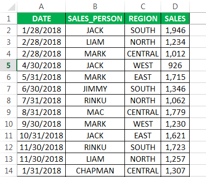
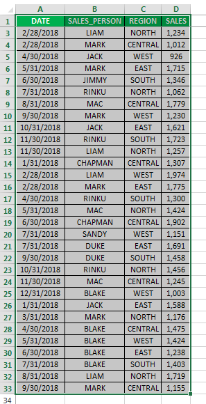
Below mentioned data contains a compilation of sales information by date, salesperson, and region. Here, we need to summarize sales data for each representative regionally in the chart.
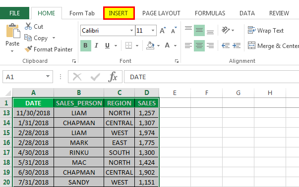
- We must first select the data range to create a PivotChart in Excel.

- Then, click the “Insert” tab within the ribbon.

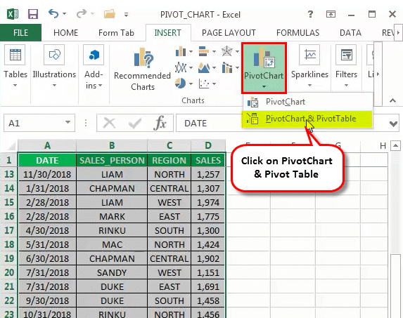
- Then, select the “PivotChart” dropdown button within the “Charts” group. So, for example, if we want only to create a PivotChart, choose “PivotChart” from the dropdown or if we are going to make both a PivotChart and PivotTable, then select “PivotChart & PivotTable” from the dropdown.

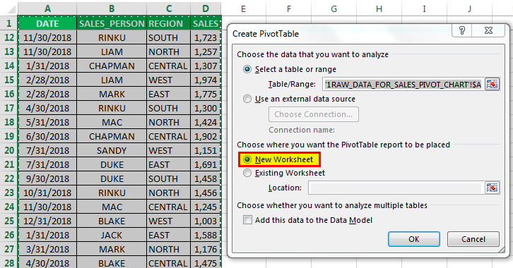
- Here, we have selected and created both a PivotChart and PivotTable. Then, make PivotChart, a dialog box appears, similar to the “Create PivotTable” dialog box. It will ask for the options: Table/Range or Use an external data source. By default, it selects “Table/Range,” which will ask where to place a PivotTable chart. Here, we always need to choose a new worksheet.

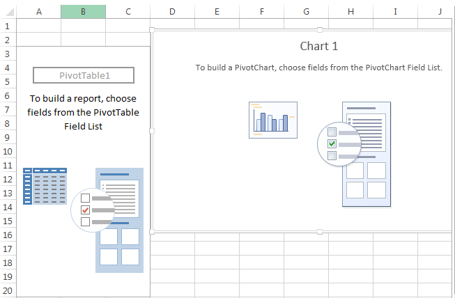
- Clicking “OK” will insert PivotChart and PivotTable into a new worksheet.

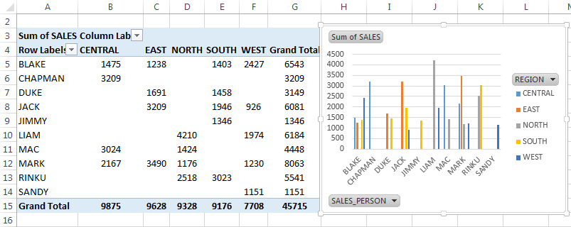
- “PivotChart Fields” task pane appears on the left, containing various fields: Filters, Axis (Categories), Legend (Series), and Values. Next, in the PivotTable Fields pane, select the “Column” fields applicable to the Pivot Table. Then, we can drag and drop, i.e., “Sales_person” to the “Rows” section, “Region” to the “Columns” section, and “Sales” to the “Values” section.

Then, the chart looks as given below.

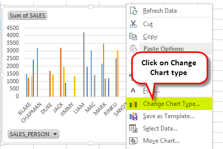
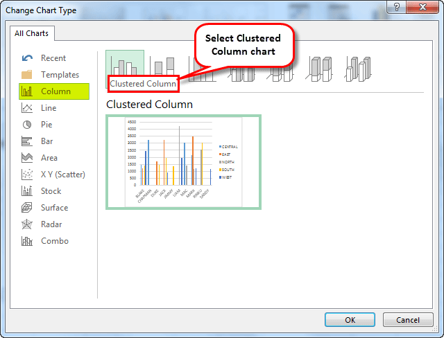
- We can name this sheet “SALES_BY_REGION” by clicking on the PivotTable. Then, we can change the chart type in the “Change Chart Type” option based on choice under the “Insert” tab. Select “PivotChart, and” the “Insert Chart” popup window appears. Under that, select the “Bar” and “Clustered” bar chart. Then, right-click on the PivotChart, and choose “Change Chart Type.”

- Under “Change Chart Type,” select “Column.” Then, select the “Clustered Column” Chart.

- Now, we can summarize the data with the help of interactive controls present across the chart. For example, when we click on the “Region” filter control, a search box appears with the list of all the regions, where we can check or uncheck boxes based on the choice.

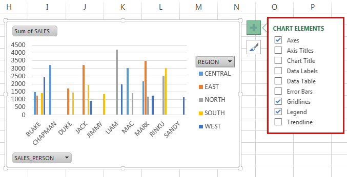
- On the corner of the chart, we have an option to format chart elements based on the choice.

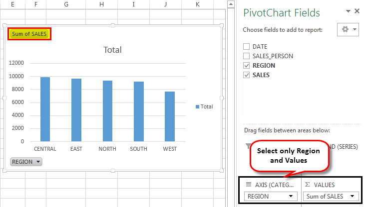
- We have an option to customize the PivotTable “Values.” By default, Excel uses the SUM function to calculate the values available in the table. Suppose we select only region values in the chart; it will display each region’s total SUM sales.

- We have an option to change the Excel chart style by clicking the “Style” icon on the corner of the chart.

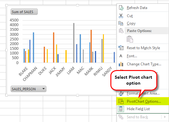
- This chart will update when we change data sets in a PivotTable. The following steps can optimize this option: right-click and select the “PivotChart Options”.


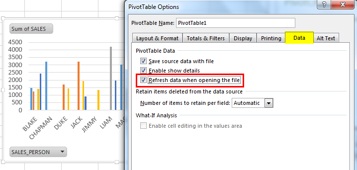
In the above chart options, go to the “Data” tab and click on the checkbox “Refresh data when opening a file.” So that refresh data gets activated.

Things to Remember
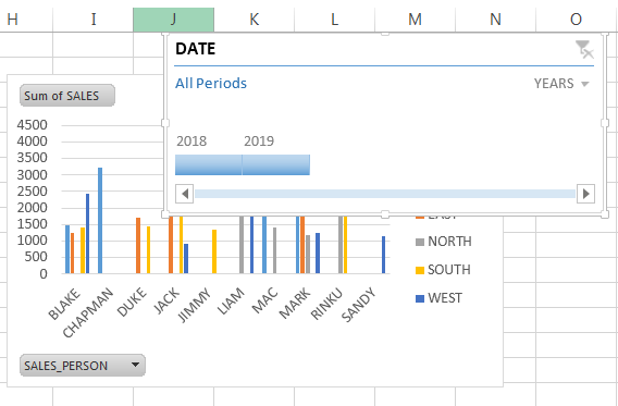
In an Excel PivotChart, we can insert a timeline to filter dates (monthly, quarterly, or yearly) in a chart to summarize sales data (This step applies when the dataset contains only date values).
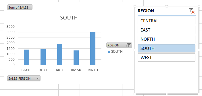
We can also use a “Slicer” with a PivotChart to filter region-wise data or other field data of the choice to summarize sales data.
- A PivotChart is a key metrics tool for monitoring company sales, finance, productivity, and other criteria.
- With the help of a PivotChart, we can identify negative trends and correct them immediately.
- One of the drawbacks of a pivot tableA Pivot Table is an Excel tool that allows you to extract data in a preferred format (dashboard/reports) from large data sets contained within a worksheet. It can summarize, sort, group, and reorganize data, as well as execute other complex calculations on it.read more is that this chart is directly linked to the datasets associated with the PivotTable, making it less flexible. Because of this, we cannot add data outside the PivotTable.
Recommended Articles
This article is a step-by-step guide to creating a PivotChart in Excel. We discuss creating a PivotChart in Excel, practical examples, and a downloadable Excel template. You may learn more about Excel from the following articles: –
- What is a Pivot Table Slicer?Pivot Table Slicer is a tool in MS Excel to filter the data present in a pivot table. The data can be presented based on various categories as it offers a way to apply the pivot table filters that dynamically change the view of the pivot table data.read more
- Types of Charts in ExcelExcel offers a variety of chart types based on your requirements. Column Charts, Line Charts, Pie Charts, Bar Charts, Area Charts, Scatter Charts, Stock Chart, and Radar Charts are the different types of charts.read more
- How to Create a Project Timeline in Excel?The project timeline is a list of tasks that must be accomplished in order to complete the project within the time frame specified. It is simply the project schedule/timetable. They usually have a start date, duration, and end date to efficiently track and complete the tasks listed.read more
- Sorting Pivot Table in ExcelThe sorting done by the pivot table is called pivot table sort. Right-click on any data to sort in the pivot tables, and you’ll see a sort option. Because pivot tables are not standard tables, the normal sort option does not apply to them.read more
A PIVOT CHART is one of the best ways to present your data in Excel.
Why I’m saying this? Well, data in a visual way not only helps the user to understand it but it also helps you to present a clearer picture of it and you can make your point clear with led efforts.
And when we talk about Excel, there is a number of charts that you use but there’s one of all those that STANDS OUT and that’s a PIVOT CHART.
If you are serious about taking your data visualization skills to the whole next level you need to learn to create a pivot chart.
And in the guide, I’ll be explaining to you all the details you need to know to understand how the pivot chart works. But before that, here are some words from Wikipedia.
Pivot Chart is the best type of graph for the analysis of data. The most useful feature is the possibility of quickly changing the portion of data displayed, like a PivotTable report. It makes the Pivot Chart ideal for the presentation of data in sales reports.

Difference Between a Pivot Chart and a Normal Chart
- A standard chart use range of cells, on the other hand, a pivot chart is based on data summarized in a pivot table.
- A pivot chart is already a dynamic chart, but you have to make changes in data to convert a standard chart into a dynamic chart.
Steps to Create a Pivot Chart in Excel
You can create a pivot chart using two ways. One is to add a pivot chart to your existing pivot table, and the other is to create a pivot chart from scratch.
1. Create a Pivot Chart from Scratch
Creating a pivot chart from scratch is as simple as creating a pivot table. All you need, is a data-sheet. Here I am using Excel 2013 but you use steps in all versions from 2007 to 2016.
- Select any of the cells in your data sheet and go to Insert Tab → Charts → Pivot Chart.

- The pop-up window will automatically select the entire data range and you have the option to choose the place where you want to insert your pivot chart.

- Click OK.
- Now, you have a blank pivot table and pivot chart in a new worksheet.

Important: When you insert a pivot chart it will automatically insert a pivot table along with it. And, if you just want to add a pivot chart, you can add your data to Power Pivot Data Model.
- In pivot chart fields, we have four components as we have in a pivot table.
- Axis: The axis in the pivot chart is as same as we have rows in our pivot table.
- Legend: Legend in the pivot chart is as same as we have columns in our pivot table.
- Values: We are using quantity as values.
- Report Filter: You can use the report filter to filter your pivot chart.

- So, here is your fully dynamic pivot chart.
2. Create a Pivot Chart from the Existing Pivot Table
If you already have a pivot table in your worksheet then you can insert a pivot chart by using these simple steps.
- Select any of the cells from your pivot table.

- Go to Insert Tab → Charts → Pivot Chart and select the chart which you want to use.

- Click Ok.
It will insert a new pivot chart in the same worksheet where you have your pivot table. And, it will use pivot table rows as the axis and columns as the legend in the pivot chart.
Important: Another smart and quick way is to use the shortcut key. Just select any of the cells in your pivot table and press F11 to insert a pivot chart.
Related: Excel Slicer
More Information about Pivot Charts
Managing a pivot chart is simple and here is some information that will help you do it smoothly.
1. Change Chart Type
When you enter a new pivot chart, you have to select the type of chart which you want to use. And, if you want to change the chart type you can use the following steps for that.
- Select your pivot chart and go to Design Tab → Type → Change Chart Type.

- Select your favorite chart type.

- Click OK.
2. Refresh a Pivot Chart
Refreshing a pivot chart is just like refreshing a pivot table. If your pivot table is refreshing automatically, then your pivot chart will also update along with that.
Method-1
- Right-click on your chart.
- And then click on pivot chart options.

- Go to the data tab and tick mark “Refresh data when open a file”.

- Click OK.
Method-2
Use below VBA code to refresh all kinds of pivot tables and pivot charts in your workbook.
Sub auto_open()
Dim PC As PivotCache
For Each PC In ActiveWorkbook.PivotCaches
PC.Refresh
Next PC
End Sub
Apart from the above code, you can use the following VBA code if you want to refresh a particular pivot table.
Sub auto_open()
ActiveSheet.ChartObjects("Chart 5").Activate
ActiveChart.PivotLayout.PivotTable.PivotCache.Refresh
End Sub
3. Filter a Pivot Chart
Just like a pivot table, you can filter your pivot chart to show some specific values. One thing is clear a pivot table and a pivot chart is connected with each other. So, when you filter a pivot table, your chart will automatically filter.
And, when you add any filter to your pivot table it will automatically add to your pivot chart and vice versa. Please follow these steps for this.
- Right-click on your pivot chart and click on “Show Field List”.

- In your pivot chart field list, drag fields in the filter area.

Important Note: By default, you have a filter option at the bottom of your pivot chart to filter axis categories.
4. Show Running Total in a Pivot Chart
In the below pivot chart, I have used a running total to show the growth throughout the period.

Enter a running total in a pivot chart is just like entering a running total in a pivot table. But we need to make some simple changes in chart formatting.
- From your pivot chart field list, drag your value field twice in the value area.

- Now, in the second field value open “Value Field Settings”.
- Go to the “show value as” tab and select running total from the drop-down.

- Click OK.
So here is your pivot chart with the running total but one more thing which we have to do to make it perfect.
- Select your primary axis and change values as per your secondary axis.

5. Move a Pivot Chart to New Sheet
Like a standard chart, you can move your Excel pivot chart to a chart sheet or any other worksheet.
To move your pivot chart.
- Select your chart and right-click on it.
- Click on the move chart and you will get a pop-up window.

- Now, you have two different options to move your chart.
- New Chart Sheet.
- Another Worksheet.
- Select the desired option and click OK.
You can also move your chart back to the original sheet using the same steps.
Some the extra tips to make better control over it.
1. Using a Slicer with a Pivot Chart to Filter
As I have already mentioned, you can use a slicer with your pivot chart.
And, the best part is that you can filter multiple pivot tables and pivot charts with a single slicer. Follow these steps.
- Select your pivot chart and go to Analyze Tab → Filter → Insert Slicer.

- Select the field which you want to use as a filter.

- Click OK.
Using a slicer is always a better option than a standard filter.
2. Insert a Timeline to Filter Dates in a Pivot Charts
If you want to filter your pivot chart using a date field then you can use a timeline instead of a slicer.
Filtering dates with a timeline is super easy.
This is like an advanced filter that you can use to filter dates in terms of days, months, quarters, and years.
- Select your pivot chart and go to Analyze Tab → Filter → Insert Timeline.

- Select your date field from the pop-up window and it will show you fields with dates.
- Click OK.
3. Present Months in a Pivot Chart by Grouping Dates
Now, let’s say you have dates in your data, and you want to create a pivot chart on monthly basis. One simple way is to add a month column in your data and use it in your pivot chart.
But, here is the twist. You can group dates in your pivot table which will further help you to create a pivot chart with months even when you don’t have months in source data.
- Go to your pivot table and select any of the cells from your date field column.
- Right-click on it and select group.

- Select the month from the pop-up window and click OK.
Sample File
Download this sample file from here to learn more.
More Charting Tips and Tutorials
- Add a Horizontal Line in a Chart in Excel
- Add a Vertical Line in a Chart in Excel
- Bullet Chart in Excel
- Dynamic Chart Range in Excel
- Dynamic Chart Title in Excel
- Interactive Charts In Excel
- Sales Funnel Chart in Excel
- How to Create a HEAT MAP in Excel
- HISTOGRAM in Excel
- Pictograph in Excel
- Milestone Chart in Excel
- People Graph in Excel
- Population Pyramid Chart in Excel
- SPEEDOMETER Chart [Gauge] in Excel
- Step Chart in Excel
- Thermometer Chart in Excel
- Tornado Chart in Excel
- Waffle Chart in Excel
Tuesday, February 16, 2016
Peltier Technical Services, Inc., Copyright © 2023, All rights reserved.
About Pivot Charts
If you select a pivot table and insert a chart, Excel inserts a pivot chart. A pivot chart is a special Excel chart, with some strengths and some limitations. I used to avoid pivot charts because of these limitations, which included not being able to hide the field buttons and not being able to resize the plot area or move axis and chart titles. But Microsoft has kept improving them, and now the few remaining limitations seem pretty reasonable given the power and constraints of pivot tables themselves.
- A pivot chart is linked to its parent pivot table. Changes to the pivot table are reflected in the pivot chart, and vice versa. If the pivot table changes size, the pivot chart changes the number of its plotted series, and changes the lengths of these series, to accommodate the updated pivot table size.
- The pivot chart has optional field buttons that allow the same filtering capabilities directly in the chart that are available to the pivot table.
- All data in the pivot table is plotted in the pivot chart, except for subtotals and grand totals. No data from outside the pivot table is allowed in the pivot chart.
- Pivot charts are plotted with category labels and series values in columns only. Pivot charts cannot be plotted by row.
- Not all chart types are available in pivot charts. Line, column, area, bar, and pie charts are available, for example, but XY scatter charts and bubble charts are not.
Often, pivot charts are exactly what is needed. Sometimes, however, a regular chart must be used. For example, you might want a scatter plot of the pivot table’s data. Or you might want to add data from another source.
My colleague Debra Dalgleish has a brief Pivot Chart Tutorial on her Contextures.com web site, as well as a FAQ page on Pivot Tables and Pivot Charts. Debra also wrote Using Pivot Tables in Microsoft Excel on this blog.
This article will answer the following common questions about pivot charts in Excel.
- How do I disconnect a pivot chart from its pivot table?
- How do I copy a pivot chart and link it to another pivot table?
- How do I convert a pivot chart into a regular chart and preserve its links to the pivot table?
The last question could be answered by Making Regular Charts from Pivot Tables. But the question is often asked by someone who has spent significant time formatting his pivot chart, and doesn’t want to lose this formatting or be forced to recreate it.
We’ll start by reviewing regular charts and how their data is handled. Then we’ll examine differences between regular charts and pivot charts. Finally we’ll investigate answers to the questions above.
Regular Charts
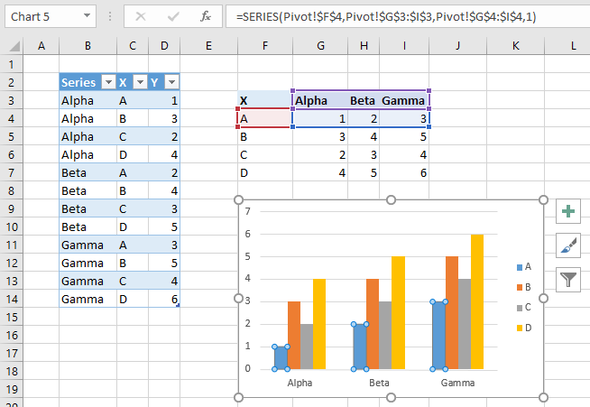
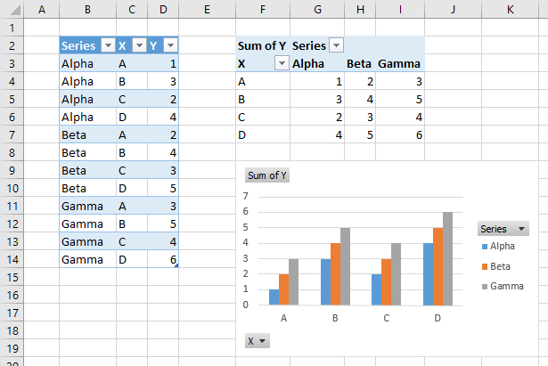
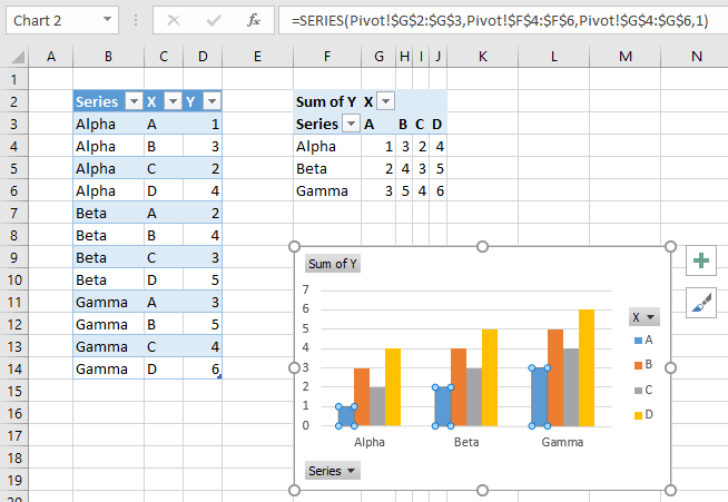
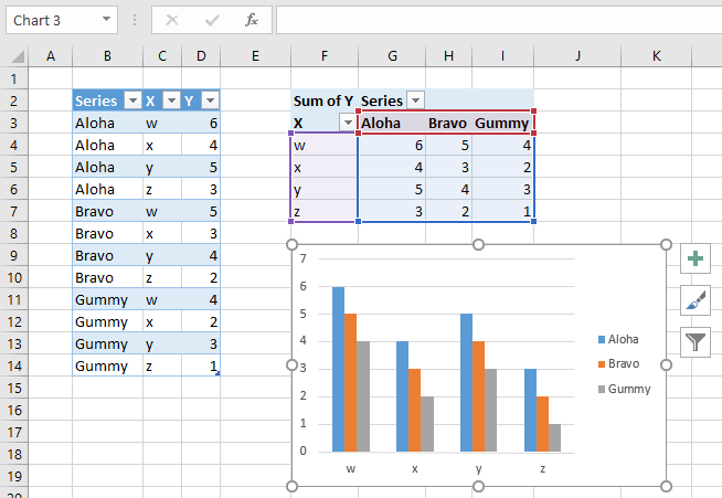
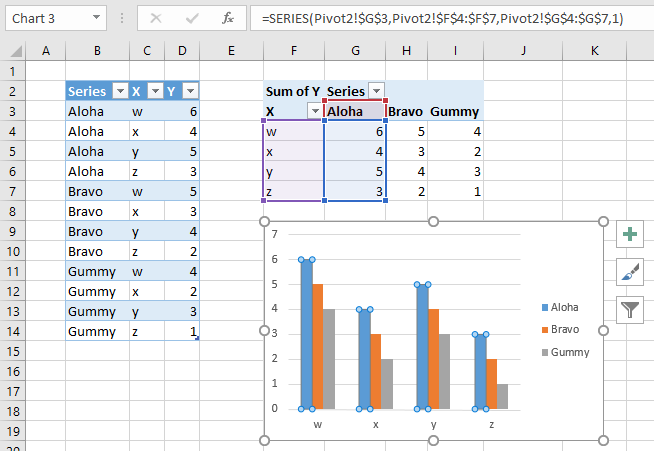
The screenshot below shows a table with some simple data located in B2:D14. The data is rearranged in F3:I7 (a pivot table could have done this). Below that is a regular Excel chart which plots the data from this second range.
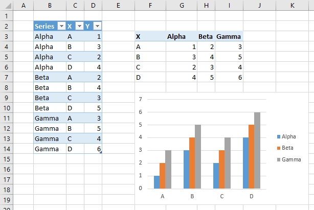
Chart Source Data Highlighting
When you select a chart that has a well-behaved* source data range, the chart’s data range is highlighted in the worksheet. The highlighting for our simple chart in Excel 2013 and 2016 is shown below: the X values (category labels) are purple, the Y values are blue, and the series names are red. You can click and drag the highlighted borders to move the chart data, and you can click and drag on the highlighted corners to resize the chart data.
*Well-behaved means that the Y values of the series are in adjacent rows or columns, in order. Y values and X values (if present) must be aligned: in the chart below, the X values and all sets of Y values all begin on the same row and all end on the same other row, and the series names are aligned with the Y values.

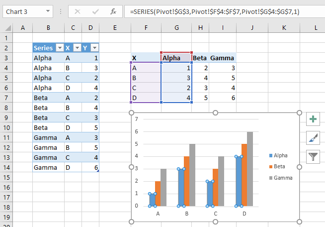
When you select a plotted series, the data for that series is highlighted in the worksheet. The highlighting for the first series of our simple chart in Excel 2013 and 2016 is shown below: the X values (category labels) are purple, the Y values are blue, and the series names are red. You can click and drag the highlighted borders to move the chart data, and you can click and drag on the highlighted corners to resize the chart data. Note that our series is plotted by columns.
Chart Series Data Highlighting
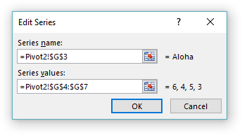
When a series is selected, you can also see the corresponding SERIES formula in the formula bar. This series formula has the following components:
- Series Name: Pivot!$G$3
- Category Labels (X Values): Pivot!$F$4:$F$7
- Y Values: Pivot!$G$4:$G$7
- Plot Order: 1
You can edit this formula in place to adjust the chart data.
Another way to adjust a chart’s data is the Select Data Source dialog. To open this dialog, click the Chart Tools > Design tab > Select Data button, or tight-click on the chart and click Select Data from the pop-up menu.
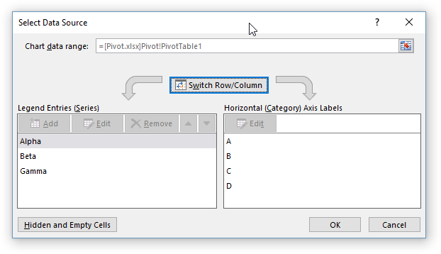
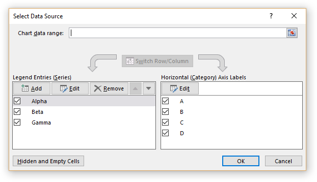
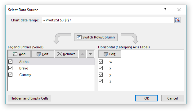
Select Source Data Dialog
Here is the Select Source Data dialog for our regular chart. The box at the top shows the entire source data, which was highlighted when we selected the entire chart. You can edit this as text, or select another source data range in a worksheet. Caveat: if your selection in the Chart data range box intersects a pivot table, your chart will be converted into a pivot chart based on that pivot table.
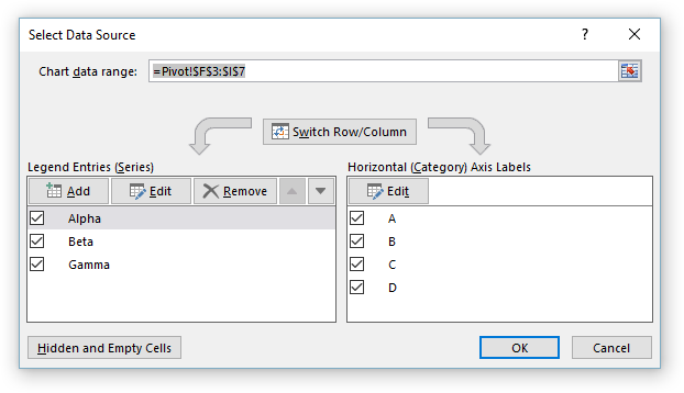
Click the Edit button under Axis Labels in the bottom right part of the dialog, and the Axis Labels dialog appears, showing the range containing the axis labels. You can edit this as text, or select another axis label range.
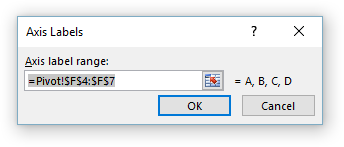
Select a series in the bottom right part of the dialog and click the corresponding Edit button, and the Edit Series dialog appears, showing the range containing the Y values. You can edit this as text, or select another range of values.

If you click the Switch Row/Column button, the same data is used as the source data, but its orientation is switched. The category axis labels become the series names, and the series names become the axis labels. Note that our chart now has four series with three points each (and three axis labels), and the red and purple highlighted regions have changed places.

When we select the first series, we see that it is now aligned in rows.
If your chart’s source data intersects a pivot table, clicking Switch Row/Column will convert your chart into a pivot chart based on that pivot table.
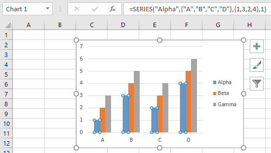
Disconnecting From Worksheet Data
Here’s a little-known debugging trick for Excel formulas. You can use the F9 function key or the Ctrl+= shortcut (hold the Ctrl key while you press the = key) to evaluate part or all of a formula in the formula bar. Fortunately this works for a SERIES formula.
If you click in the formula bar and click F9 or Ctrl+=, every section of the formula is evaluated (and the links are disconnected), as shown in this before-and-after screenshot.
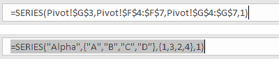
Click Esc to restore the original formula, or Enter to keep the evaluated formula.
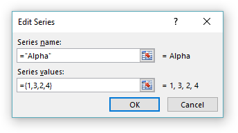
If you select just part of a formula and then click F9 or Ctrl+=, just the selected part of the formula is evaluated. In this screenshot, the Y value range of G4:G7 is converted to the array {1;3;2;4}.
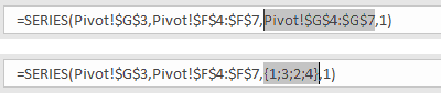
To unlink a regular chart from its worksheet data, select each series, click in the formula bar, and press the F9 key.
Copying the Chart
You can copy a chart and paste it anywhere in the same workbook, even onto a different worksheet, and nothing happens to the chart. It shows the same data that it was linked to (on the original sheet), and the series formulas still link back to the original data. This is familiar, expected behavior, although when you want to link the chart to the data on its new parent worksheet, it’s not so welcome. But see Make a Copied Chart Link to New Data if that’s what you need to do.
When you copy a regular chart to a new workbook, it still points back to the original data, which in the SERIES formula is referenced to the original workbook as well as the original worksheet, as “[Pivot.xlsx]Pivot”. So the regular chart behaves exactly as expected.
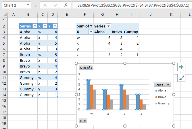
The screenshot below shows a table with the same simple data located in B2:D14. A pivot table in F2:I7 has rearranged the data. Below the pivot table is an Excel pivot chart which plots the data from the pivot table. Note the field buttons in the pivot chart, corresponding to the controls in the pivot table.
We can hide the field buttons (Pivot Chart Tools > Analyze ribbon tab > Field Buttons) and the chart will look just like our regular chart. But it still has the capabilities and limitations of a pivot chart.
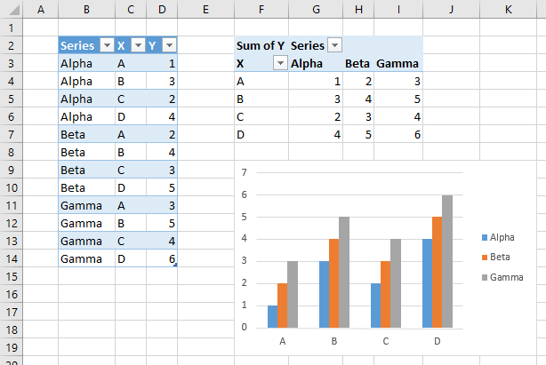
Chart Source Data Highlighting
When the pivot chart is selected, no chart data highlights appear in the worksheet.
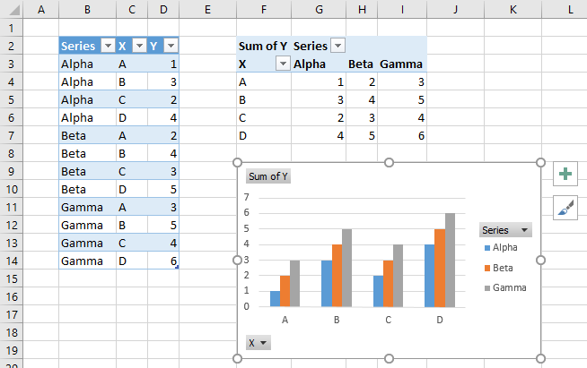
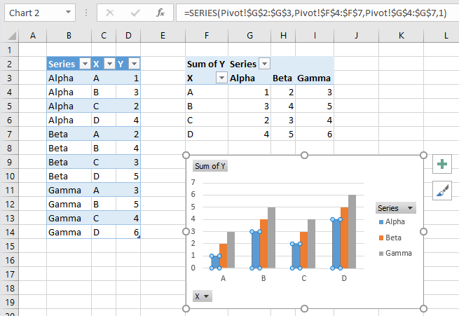
Chart Series Data Highlighting
When a series is selected in the pivot chart, no series data highlights appear in the worksheet. The SERIES formula appears in the formula bar, but you cannot edit the series data by editing the series formula. You can only change the series plot order by changing the last parameter in the series formula.
Select Source Data Dialog
Here is the Select Source Data dialog for our pivot chart. The box at the top shows that the source data is our pivot table; this cannot be changed. The axis labels cannot be edited, nor can the series values be edited.
If you click the Switch Row/Column button, the chart changes its appearance to match how our regular chart changed: three series of four categories becomes four series of three categories. But the chart’s data orientation didn’t change, because pivot charts can only plot columns of data. Instead, Excel switched the fields in the rows area of the pivot table with those in the columns area. The X and Series field buttons in the chart have changed places as well.
The series formula shows that the first series of our pivot chart is still plotted by column, with the category labels in column F and Y values in column G.
Disconnecting From Worksheet Data
Excel does not let you evaluate part or all of a pivot chart’s SERIES formula using the F9 or Ctrl+= trick, so you can’t use it to disconnect the pivot chart from its pivot table.
Copying the Chart
You can copy a pivot chart and paste it anywhere in the same workbook, even onto a different worksheet, and nothing happens to the chart. It shows the same data that it was linked to (in the original pivot tables), and the series formulas still link back to this pivot table.
Answering Those Questions
How do I disconnect a pivot chart from its pivot table?
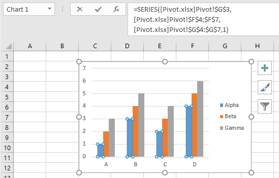
Interesting things happen when you copy a pivot chart to a different workbook. The first thing you may notice is that the field buttons have disappeared, because the pivot chart has been converted to a regular chart. The second thing you’ll notice, if you check out the SERIES formula, is that the links to worksheet ranges have been changed into literal arrays of strings and numbers, as if we used our F9 (Ctrl+=) trick to evaluate the formula.
There’s the answer to our first question, how to unlink a pivot chart from its pivot table. Simply copy the pivot chart to a different workbook. Once the links are broken, you can copy it anywhere, even into the original workbook, and it will remain disconnected from the pivot table.
How do I copy a pivot chart and link it to another pivot table?
In the screenshot below, I’ve copied my unlinked chart and pasted it into the original workbook, in a different worksheet with a different Table of data and a different Pivot Table. As noted above, it’s still disconnected.
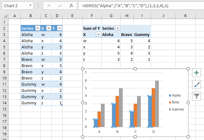
Here is the Select Source Data dialog for our unlinked chart. The Chart Data Range box at the top is empty, because the chart’s data is hard-coded into the chart’s SERIES formulas. You can click in the box and select a data range from the worksheet.
If you select a cell or range that overlaps with a pivot table and click OK, the chart will become a pivot chart and use the data from the selected pivot table. In the screenshot below the chart now has field buttons, so we know it has been converted into a pivot chart. The SERIES formula shows links to the data in the pivot table.
There’s the answer to our second question, how to copy a pivot chart but link it to a new pivot table. Copy the pivot chart to a different workbook to disconnect it from the first pivot table, then copy the chart to the sheet with the second pivot table, then use the Select Data dialog and select the new pivot table in the Chart Data Range box.
How do I convert a pivot chart into a regular chart and preserve its links to the pivot table?
If we avoid the Chart Data Range box, we can still use the Select Data Source dialog to reconstruct links to the pivot table data. This is essentially the technique in Making Regular Charts from Pivot Tables, but we’re using the pivot chart which may have had custom formats applied.
Under Horizontal (Category) Axis Labels, click Edit, and the Axis Labels mini-dialog will appear, showing the literal array of labels.
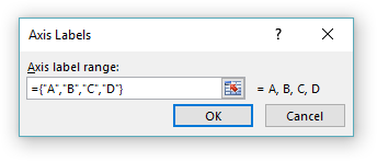
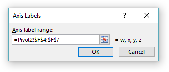
You can clear the box and select the axis label range from the worksheet using your mouse. Then click OK.
Now under Legend Entries (Series), select the first series from list, and click Edit. The Edit Series mini-dialog appears with the series name as a string, and the series values as a literal array of numbers.
You can clear each box and select the cell containing the series name and the column of cells containing the series values. Click OK, then repeat for the rest of the series in the chart.
The Select Data Source dialog now looks like this, with the Chart Data Range box displaying the range containing all of the pivot table data. Don’t click in this box, and don’t click Switch Row/Column, or your chart will become a pivot chart.
Click OK, and notice how the chart now plots the pivot table data. The data is highlighted in the worksheet, and the chart has no field buttons, because it remains a regular chart.
Selecting a single series shows the data is plotted by column, but again, the series highlights verify that the chart is not a pivot chart.
And this is the answer to our last question, how to convert our pivot chart to a regular chart but maintain links to the pivot table’s data. Actually, I’ve linked it here to a new pivot table, but I could link it to the original pivot table in the same way. Strictly speaking, this approach didn’t actually maintain the links, as we had to reconstruct them. There is no way to maintain the links while converting the pivot chart into a regular chart.
This Pivot Charts in Excel tutorial is Suitable for users of Excel 2010/2013/2016/2019 and Microsoft 365.
Objective
Create an interactive Pivot Chart in Excel from a raw dataset and customize it to suit your needs.
What is a Pivot Chart?
Whenever I hear the word ‘Pivot’ I immediately think about that scene in ‘Friends’. Ross, Rachel and Chandler struggling to lift a couch up a very narrow stairway. Fortunately, Pivot in the context of Excel is a much simpler affair and not quite as shouty. Unless you accidentally delete your Pivot Chart then all bets are off.
Pivot Charts are used in conjunction with PivotTables. A PivotTable helps you summarize your raw data and extract meaning from a large dataset. However, sometimes it’s still hard to see the big picture. A Pivot Chart in Excel can instantly help you visualize large datasets, make better decisions and tell the story of your data. Every element of a Pivot Chart can be modified and customized and with useful tools like Slicers, it makes viewing your data against different criteria simple and easy for everyone.
In short, Pivot Charts are awesome and definitely something you need to have in your Excel toolkit!
There is a common misconception that in order to create a Pivot Chart, you must first create a PivotTable. This isn’t necessarily the case. You absolutely can create a PivotTable and then create a Pivot Chart but you don’t have to.
However, it is very important that prior to creating a Pivot Chart (or a PivotTable for that matter), that you ‘clean’ your data. This is especially important if you are using a dataset that you didn’t create, i.e. imported from a database, another Excel file etc. Cleaning data is the process of removing errors, blank rows, duplicates and also checking for consistency in your data. If you do not do this, any results you see in your Pivot Chart could be inaccurate.
To learn the different techniques for cleaning data in Excel, check out the following blogs:
Microsoft – Top ten ways to clean your data
Trump Excel – 10 Super Neat Ways to Clean Data in Excel Spreadsheets
Simon Sez IT – Data Cleaning in Excel in 1 Hour
In this example, we are starting out with a large dataset (21,574 rows), that has already been cleaned and formatted as a table. The data is Sales data for two different stores in the UK. The table has been named ‘SalesData’.
Method
1. Creating a Pivot Chart Open the Excel workbook that contains the data you want to analyze and ensure your mouse is clicked on a cell contained within your data.
2. Click Insert > Pivot Chart

The ‘Create Pivot Chart’ dialog box will open. You need to specify the cell range that contains the data to be used in the Pivot Chart in the ‘Table/Range’ field. If you have not named your data range, you can simply select the cell range manually. In my example, I named the data range ‘SalesData’.
Next, specify where you want to create the Pivot Chart. I always recommend separating the raw data from the Pivot Chart and putting it on a ‘New Worksheet’.

3. Click OK
A new worksheet tab will be created. On the left is a blank PivotTable, in the middle a blank Pivot Chart an on the right are the Pivot Chart fields.
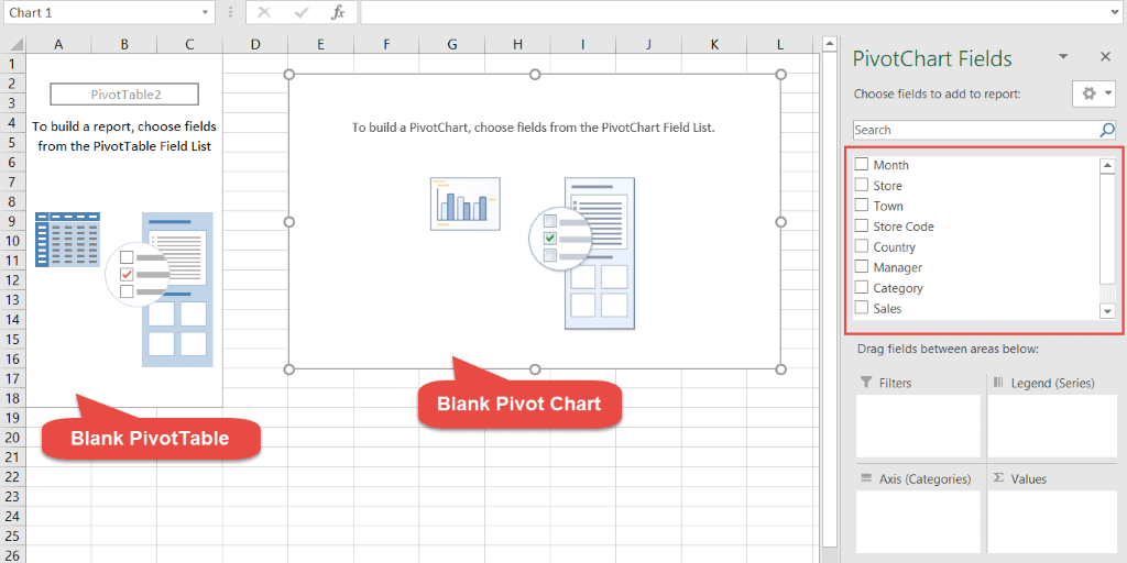
The Pivot Chart fields correspond to the column headings in the raw data worksheet.
To build a Pivot Chart, drag any of the fields and drop into one of the four areas at the bottom. Which field you drag and drop into which area will determine how your data is displayed in the Pivot Chart.

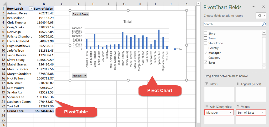
For example, I would like to see a summary of the total number of sales for all store managers.
- Drag the ‘Sales’ field to the ‘Values’ area
- Drag the ‘Manager’ field to the ‘Axis(Categories)’ area
Now, I want to see a summary of the data, broken down by store.
- Drag the ‘Store’ field to the ‘Legend (Series)’ area.

Next, I want to see a summary of the sales by category.
- Untick the ‘Store’ and the ‘Manager’ field in the Pivot Chart fields list to remove them.
- Drag the ‘Category’ field to the ‘Axis Categories’ area.

This is a basic Pivot Chart. Fields can added or removed depending on how you want the Pivot Chart to display the data.
Formatting Pivot Charts
There are many utilities available in Excel to format Pivot Charts. Click on the Pivot Chart to see the ‘PivotChart Tools’ contextual ribbon.
The Analyze tab
The Analyze tab contains tools to help you interpret your Pivot Chart. Give your chart a name to make it easy to identify. Add Slicers and Timelines to filter the Pivot Chart. Change your data source, or refresh the current data source if it’s been updated. Move the Pivot Chart or create formulas using calculated fields.

The Design tab
The Design tab contains tools to help you format and label your Pivot Chart. Add chart elements such as a title, a legend or axis labels. Modify the layout and change the color of the chart. Select a different chart style or change the chart type or switch the row and column data.

The Format tab
The format tab contains tools to format every element of your Pivot Chart. Change the fill color, the outline color or add effects.

In this example, a legend has been added to show the two stores represented in the Pivot Chart. Horizontal and Vertical Axis titles have been added. The chart style has been changed and the chart area has been formatted.

Adding Interactive Elements
Slicers and Timelines enable you to filter the Pivot Chart and target the information of interest to you.
Add a Slicer
- Click on the Pivot Chart
- From the PivotTable Tools ribbon, select the Analyze tab
- Click Insert Slicer
- Select the field or fields you want to use to filter the Pivot Chart
- Click OK

Add a Timeline
Timelines are a Slicer specifically for data formatted as a date. Using a Timeline Slicer, you can display your Pivot Chart data for a specific date range.
- Click on the Pivot Chart
- From the PivotTable Tools ribbon, select the Analyze tab
- Click Inset Timeline
- Select the date field you want to use to filter the Pivot Chart
- Click OK

To clear filter selections for Slicers and Timelines, click the ‘Clear Filter’ icon
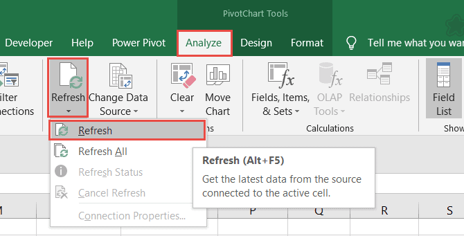
Updating a Pivot Chart
It’s more than likely that your raw data will change at some point. New data will be added so its important to know how to keep your Pivot Chart updated.
- Add the new rows or columns to the raw data table
- Click on the Pivot Chart
- From the PivotTable Tools ribbon, select the Analyze tab
- Click Refresh or Refresh All
Video Tutorial
To see Pivot Charts in action, please watch the following video tutorial.
For more Free Excel tutorials from Simon Sez IT. Take a look at our Excel Resource Center.
To learn Excel with Simon Sez IT. Take a look at the Excel courses we have available.
Deborah Ashby

Deborah Ashby is a TAP Accredited IT Trainer, specializing in the design, delivery, and facilitation of Microsoft courses both online and in the classroom.She has over 11 years of IT Training Experience and 24 years in the IT Industry. To date, she’s trained over 10,000 people in the UK and overseas at companies such as HMRC, the Metropolitan Police, Parliament, SKY, Microsoft, Kew Gardens, Norton Rose Fulbright LLP.She’s a qualified MOS Master for 2010, 2013, and 2016 editions of Microsoft Office and is COLF and TAP Accredited and a member of The British Learning Institute.