
The IF function allows you to make a logical comparison between a value and what you expect by testing for a condition and returning a result if True or False.
-
=IF(Something is True, then do something, otherwise do something else)
So an IF statement can have two results. The first result is if your comparison is True, the second if your comparison is False.
IF statements are incredibly robust, and form the basis of many spreadsheet models, but they are also the root cause of many spreadsheet issues. Ideally, an IF statement should apply to minimal conditions, such as Male/Female, Yes/No/Maybe, to name a few, but sometimes you might need to evaluate more complex scenarios that require nesting* more than 3 IF functions together.
* “Nesting” refers to the practice of joining multiple functions together in one formula.
Use the IF function, one of the logical functions, to return one value if a condition is true and another value if it’s false.
Syntax
IF(logical_test, value_if_true, [value_if_false])
For example:
-
=IF(A2>B2,»Over Budget»,»OK»)
-
=IF(A2=B2,B4-A4,»»)
|
Argument name |
Description |
|
logical_test (required) |
The condition you want to test. |
|
value_if_true (required) |
The value that you want returned if the result of logical_test is TRUE. |
|
value_if_false (optional) |
The value that you want returned if the result of logical_test is FALSE. |
Remarks
While Excel will allow you to nest up to 64 different IF functions, it’s not at all advisable to do so. Why?
-
Multiple IF statements require a great deal of thought to build correctly and make sure that their logic can calculate correctly through each condition all the way to the end. If you don’t nest your formula 100% accurately, then it might work 75% of the time, but return unexpected results 25% of the time. Unfortunately, the odds of you catching the 25% are slim.
-
Multiple IF statements can become incredibly difficult to maintain, especially when you come back some time later and try to figure out what you, or worse someone else, was trying to do.
If you find yourself with an IF statement that just seems to keep growing with no end in sight, it’s time to put down the mouse and rethink your strategy.
Let’s look at how to properly create a complex nested IF statement using multiple IFs, and when to recognize that it’s time to use another tool in your Excel arsenal.
Examples
Following is an example of a relatively standard nested IF statement to convert student test scores to their letter grade equivalent.

-
=IF(D2>89,»A»,IF(D2>79,»B»,IF(D2>69,»C»,IF(D2>59,»D»,»F»))))
This complex nested IF statement follows a straightforward logic:
-
If the Test Score (in cell D2) is greater than 89, then the student gets an A
-
If the Test Score is greater than 79, then the student gets a B
-
If the Test Score is greater than 69, then the student gets a C
-
If the Test Score is greater than 59, then the student gets a D
-
Otherwise the student gets an F
This particular example is relatively safe because it’s not likely that the correlation between test scores and letter grades will change, so it won’t require much maintenance. But here’s a thought – what if you need to segment the grades between A+, A and A- (and so on)? Now your four condition IF statement needs to be rewritten to have 12 conditions! Here’s what your formula would look like now:
-
=IF(B2>97,»A+»,IF(B2>93,»A»,IF(B2>89,»A-«,IF(B2>87,»B+»,IF(B2>83,»B»,IF(B2>79,»B-«, IF(B2>77,»C+»,IF(B2>73,»C»,IF(B2>69,»C-«,IF(B2>57,»D+»,IF(B2>53,»D»,IF(B2>49,»D-«,»F»))))))))))))
It’s still functionally accurate and will work as expected, but it takes a long time to write and longer to test to make sure it does what you want. Another glaring issue is that you’ve had to enter the scores and equivalent letter grades by hand. What are the odds that you’ll accidentally have a typo? Now imagine trying to do this 64 times with more complex conditions! Sure, it’s possible, but do you really want to subject yourself to this kind of effort and probable errors that will be really hard to spot?
Tip: Every function in Excel requires an opening and closing parenthesis (). Excel will try to help you figure out what goes where by coloring different parts of your formula when you’re editing it. For instance, if you were to edit the above formula, as you move the cursor past each of the ending parentheses “)”, its corresponding opening parenthesis will turn the same color. This can be especially useful in complex nested formulas when you’re trying to figure out if you have enough matching parentheses.
Additional examples
Following is a very common example of calculating Sales Commission based on levels of Revenue achievement.

-
=IF(C9>15000,20%,IF(C9>12500,17.5%,IF(C9>10000,15%,IF(C9>7500,12.5%,IF(C9>5000,10%,0)))))
This formula says IF(C9 is Greater Than 15,000 then return 20%, IF(C9 is Greater Than 12,500 then return 17.5%, and so on…
While it’s remarkably similar to the earlier Grades example, this formula is a great example of how difficult it can be to maintain large IF statements – what would you need to do if your organization decided to add new compensation levels and possibly even change the existing dollar or percentage values? You’d have a lot of work on your hands!
Tip: You can insert line breaks in the formula bar to make long formulas easier to read. Just press ALT+ENTER before the text you want to wrap to a new line.
Here is an example of the commission scenario with the logic out of order:

Can you see what’s wrong? Compare the order of the Revenue comparisons to the previous example. Which way is this one going? That’s right, it’s going from bottom up ($5,000 to $15,000), not the other way around. But why should that be such a big deal? It’s a big deal because the formula can’t pass the first evaluation for any value over $5,000. Let’s say you’ve got $12,500 in revenue – the IF statement will return 10% because it is greater than $5,000, and it will stop there. This can be incredibly problematic because in a lot of situations these types of errors go unnoticed until they’ve had a negative impact. So knowing that there are some serious pitfalls with complex nested IF statements, what can you do? In most cases, you can use the VLOOKUP function instead of building a complex formula with the IF function. Using VLOOKUP, you first need to create a reference table:

-
=VLOOKUP(C2,C5:D17,2,TRUE)
This formula says to look for the value in C2 in the range C5:C17. If the value is found, then return the corresponding value from the same row in column D.

-
=VLOOKUP(B9,B2:C6,2,TRUE)
Similarly, this formula looks for the value in cell B9 in the range B2:B22. If the value is found, then return the corresponding value from the same row in column C.
Note: Both of these VLOOKUPs use the TRUE argument at the end of the formulas, meaning we want them to look for an approxiate match. In other words, it will match the exact values in the lookup table, as well as any values that fall between them. In this case the lookup tables need to be sorted in Ascending order, from smallest to largest.
VLOOKUP is covered in much more detail here, but this is sure a lot simpler than a 12-level, complex nested IF statement! There are other less obvious benefits as well:
-
VLOOKUP reference tables are right out in the open and easy to see.
-
Table values can be easily updated and you never have to touch the formula if your conditions change.
-
If you don’t want people to see or interfere with your reference table, just put it on another worksheet.
Did you know?
There is now an IFS function that can replace multiple, nested IF statements with a single function. So instead of our initial grades example, which has 4 nested IF functions:
-
=IF(D2>89,»A»,IF(D2>79,»B»,IF(D2>69,»C»,IF(D2>59,»D»,»F»))))
It can be made much simpler with a single IFS function:
-
=IFS(D2>89,»A»,D2>79,»B»,D2>69,»C»,D2>59,»D»,TRUE,»F»)
The IFS function is great because you don’t need to worry about all of those IF statements and parentheses.
Need more help?
You can always ask an expert in the Excel Tech Community or get support in the Answers community.
Related Topics
Video: Advanced IF functions
IFS function (Microsoft 365, Excel 2016 and later)
The COUNTIF function will count values based on a single criteria
The COUNTIFS function will count values based on multiple criteria
The SUMIF function will sum values based on a single criteria
The SUMIFS function will sum values based on multiple criteria
AND function
OR function
VLOOKUP function
Overview of formulas in Excel
How to avoid broken formulas
Detect errors in formulas
Logical functions
Excel functions (alphabetical)
Excel functions (by category)
This Excel tutorial explains how to nest the Excel IF function with syntax and examples.
Description
The IF function is a built-in function in Excel that is categorized as a Logical Function. It can be used as a worksheet function (WS) in Excel. As a worksheet function, the IF function can be entered as part of a formula in a cell of a worksheet.
It is possible to nest multiple IF functions within one Excel formula. You can nest up to 7 IF functions to create a complex IF THEN ELSE statement.
TIP: If you have Excel 2016, try the new IFS function instead of nesting multiple IF functions.
Syntax
The syntax for the nesting the IF function is:
IF( condition1, value_if_true1, IF( condition2, value_if_true2, value_if_false2 ))
This would be equivalent to the following IF THEN ELSE statement:
IF condition1 THEN
   value_if_true1
ELSEIF condition2 THEN
   value_if_true2
ELSE
   value_if_false2
END IF
Parameters or Arguments
- condition
- The value that you want to test.
- value_if_true
- The value that is returned if condition evaluates to TRUE.
- value_if_false
- The value that is return if condition evaluates to FALSE.
Example (as Worksheet Function)
Let’s look at an example to see how you would use a nested IF and explore how to use the nested IF function as a worksheet function in Microsoft Excel:
Based on the Excel spreadsheet above, the following Nested IF examples would return:
=IF(A1="10x12",120,IF(A1="8x8",64,IF(A1="6x6",36)))
Result: 120

=IF(A2="10x12",120,IF(A2="8x8",64,IF(A2="6x6",36)))
Result: 64

=IF(A3="10x12",120,IF(A3="8x8",64,IF(A3="6x6",36)))
Result: 36
TIP: When nesting multiple IF functions, DO NOT start the second IF function with = sign.
Incorrect formula:
=IF(A1=2,»Hello»,=IF(A1=3,»Goodbye»,0))
Correct formula
=IF(A1=2,»Hello»,IF(A1=3,»Goodbye»,0))
Frequently Asked Questions
Question: In Microsoft Excel, I need to write a formula that works this way:
If (cell A1) is less than 20, then multiply by 1,
If it is greater than or equal to 20 but less than 50, then multiply by 2
If its is greater than or equal to 50 and less than 100, then multiply by 3
And if it is great or equal to than 100, then multiply by 4
Answer: You can write a nested IF statement to handle this. For example:
=IF(A1<20, A1*1, IF(A1<50, A1*2, IF(A1<100, A1*3, A1*4)))
Question:In Excel, I need a formula in cell C5 that does the following:
IF A1+B1 <= 4, return $20
IF A1+B1 > 4 but <= 9, return $35
IF A1+B1 > 9 but <= 14, return $50
IF A1+B1 > 15, return $75
Answer:In cell C5, you can write a nested IF statement that uses the AND function as follows:
=IF((A1+B1)<=4,20,IF(AND((A1+B1)>4,(A1+B1)<=9),35,IF(AND((A1+B1)>9,(A1+B1)<=14),50,75)))
Question: In Microsoft Excel, I need a formula for the following:
IF cell A1= PRADIP then value will be 100
IF cell A1= PRAVIN then value will be 200
IF cell A1= PARTHA then value will be 300
IF cell A1= PAVAN then value will be 400
Answer: You can write an IF statement as follows:
=IF(A1="PRADIP",100,IF(A1="PRAVIN",200,IF(A1="PARTHA",300,IF(A1="PAVAN",400,""))))
Question: In Microsoft Excel, I want to calculate following using an «if» formula:
if A1<100,000 then A1*.1% but minimum 25
and if A1>1,000,000 then A1*.01% but maximum 5000
Answer: You can write a nested IF statement that uses the MAX function and the MIN function as follows:
=IF(A1<100000,MAX(25,A1*0.1%),IF(A1>1000000,MIN(5000,A1*0.01%),""))
Question:I have Excel 2000. If cell A2 is greater than or equal to 0 then add to C1. If cell B2 is greater than or equal to 0 then subtract from C1. If both A2 and B2 are blank then equals C1. Can you help me with the IF function on this one?
Answer: You can write a nested IF statement that uses the AND function and the ISBLANK function as follows:
=IF(AND(ISBLANK(A2)=FALSE,A2>=0),C1+A2, IF(AND(ISBLANK(B2)=FALSE,B2>=0),C1-B2, IF(AND(ISBLANK(A2)=TRUE, ISBLANK(B2)=TRUE),C1,"")))
Question:How would I write this equation in Excel? If D12<=0 then D12*L12, If D12 is > 0 but <=600 then D12*F12, If D12 is >600 then ((600*F12)+((D12-600)*E12))
Answer: You can write a nested IF statement as follows:
=IF(D12<=0,D12*L12,IF(D12>600,((600*F12)+((D12-600)*E12)),D12*F12))
Question:I have read your piece on nested IFs in Excel, but I still cannot work out what is wrong with my formula please could you help? Here is what I have:
=IF(63<=A2<80,1,IF(80<=A2<95,2,IF(A2=>95,3,0)))
Answer: The simplest way to write your nested IF statement based on the logic you describe above is:
=IF(A2>=95,3,IF(A2>=80,2,IF(A2>=63,1,0)))
This formula will do the following:
If A2 >= 95, the formula will return 3 (first IF function)
If A2 < 95 and A2 >= 80, the formula will return 2 (second IF function)
If A2 < 80 and A2 >= 63, the formula will return 1 (third IF function)
If A2 < 63, the formula will return 0
Question:I’m very new to the Excel world, and I’m trying to figure out how to set up the proper formula for an If/then cell.
What I’m trying for is:
If B2’s value is 1 to 5, then multiply E2 by .77
If B2’s value is 6 to 10, then multiply E2 by .735
If B2’s value is 11 to 19, then multiply E2 by .7
If B2’s value is 20 to 29, then multiply E2 by .675
If B2’s value is 30 to 39, then multiply E2 by .65
I’ve tried a few different things thinking I was on the right track based on the IF, and AND function tutorials here, but I can’t seem to get it right.
Answer:To write your IF formula, you need to nest multiple IF functions together in combination with the AND function.
The following formula should work for what you are trying to do:
=IF(AND(B2>=1, B2<=5), E2*0.77, IF(AND(B2>=6, B2<=10), E2*0.735, IF(AND(B2>=11, B2<=19), E2*0.7, IF(AND(B2>=20, B2<=29), E2*0.675, IF(AND(B2>=30, B2<=39), E2*0.65,"")))))
As one final component of your formula, you need to decide what to do when none of the conditions are met. In this example, we have returned «» when the value in B2 does not meet any of the IF conditions above.
Question:I have a nesting OR function problem:
My nonworking formula is:
=IF(C9=1,K9/J7,IF(C9=2,K9/J7,IF(C9=3,K9/L7,IF(C9=4,0,K9/N7))))
In Cell C9, I can have an input of 1, 2, 3, 4 or 0. The problem is on how to write the «or» condition when a «4 or 0» exists in Column C. If the «4 or 0» conditions exists in Column C I want Column K divided by Column N and the answer to be placed in Column M and associated row
Answer:You should be able to use the OR function within your IF function to test for C9=4 OR C9=0 as follows:
=IF(C9=1,K9/J7,IF(C9=2,K9/J7,IF(C9=3,K9/L7,IF(OR(C9=4,C9=0),K9/N7))))
This formula will return K9/N7 if cell C9 is either 4 or 0.
Question:In Excel, I am trying to create a formula that will show the following:
If column B = Ross and column C = 8 then in cell AB of that row I want it to show 2013, If column B = Block and column C = 9 then in cell AB of that row I want it to show 2012.
Answer:You can create your Excel formula using nested IF functions with the AND function.
=IF(AND(B1="Ross",C1=8),2013,IF(AND(B1="Block",C1=9),2012,""))
This formula will return 2013 as a numeric value if B1 is «Ross» and C1 is 8, or 2012 as a numeric value if B1 is «Block» and C1 is 9. Otherwise, it will return blank, as denoted by «».
Question:In Excel, I really have a problem looking for the right formula to express the following:
If B1=0, C1 is equal to A1/2
If B1=1, C1 is equal to A1/2 times 20%
If D1=1, C1 is equal to A1/2-5
I’ve been trying to look for any same expressions in your site. Please help me fix this.
Answer:In cell C1, you can use the following Excel formula with 3 nested IF functions:
=IF(B1=0,A1/2, IF(B1=1,(A1/2)*0.2, IF(D1=1,(A1/2)-5,"")))
Please note that if none of the conditions are met, the Excel formula will return «» as the result.
Question:In Excel, what have I done wrong with this formula?
=IF(OR(ISBLANK(C9),ISBLANK(B9)),"",IF(ISBLANK(C9),D9-TODAY(), "Reactivated"))
I want to make an event that if B9 and C9 is empty, the value would be empty. If only C9 is empty, then the output would be the remaining days left between the two dates, and if the two cells are not empty, the output should be the string ‘Reactivated’.
The problem with this code is that IF(ISBLANK(C9),D9-TODAY() is not working.
Answer:First of all, you might want to replace your OR function with the AND function, so that your Excel IF formula looks like this:
=IF(AND(ISBLANK(C9),ISBLANK(B9)),"",IF(ISBLANK(C9),D9-TODAY(),"Reactivated"))
Next, make sure that you don’t have any abnormal formatting in the cell that contains the results. To be safe, right click on the cell that contains the formula and choose Format Cells from the popup menu. When the Format Cells window appears, select the Number tab. Choose General as the format and click on the OK button.
Question:I’m looking to return an answer from a number ‘n’ that needs to satisfy a certain range criteria. New stamp duty calculators for UK property set bands for percentage stamp duty as follows:
0-125000 =0%
125001-250000 =2%
250001-975000 =5%
975001-1500000 =10%
>1500000 =12%
I realise it’s probably an ‘IF(AND)’ function but I appear to require too many arguments. Can you help?
Answer:You can create this formula using nested IF functions. We will assume that your number ‘n’ resides in cell B1. You can create your formula as follows:
=IF(B1>1500000,B1*0.12, IF(B1>=975001,B1*0.1, IF(B1>=250001,B1*0.05, IF(B1>=125001,B1*0.02,0))))
Since your IF conditions will cover all numbers in the range of 0 to >1500000, it is easiest to work backwards starting with the >1500000 condition. Excel will evaluate each condition and stop when a condition is TRUE. This is why we can simplify the formulas within the nested IF functions, instead of testing ranges using two comparisons such as AND(B1>=125001, B1<=250000).
Question:Let’s expand the last question further and assume that we need to calculate percentages based on tiers (not just on the value as whole):
0-125000 =0%
125001-250000 =2%
250001-975000 =5%
975001-1500000 =10%
>1500000 =12%
Say I enter 1,000,000 in B1. The first 125,000 attracts 0%, the next 125,000 to 250,000 attracts 2%, and so on.
Answer:This adds a level of complexity to our formula since we have to calculate each range of the number using a different percentage.
We can create this solution with the following formula:
=IF(B1<=125000,0, IF(B1<=250000,(B1-125000)*0.02, IF(B1<=975000,(125000*0.02)+((B1-250000)*0.05), IF(B1<=1500000,(125000*0.02)+(725000*0.05)+((B1-975000)*0.1), (125000*0.02)+(725000*0.05)+(525000*0.1)+((B1-1500000)*0.12)))))
If the value was below 125,000, the formula would return 0.
If the value is between 125,001 and 250,000, it would calculate 0% on the first 125,000 and 2% on the remainder.
If the value is between 250,001 and 250,001, it would calculate 0% on the first 125,000, 2% on the next 125,000 and 5% on the remainder.
And so on….
In Excel, the Nested IF function means we can use another logical or conditional function with the IF function to test more than one condition. For example, suppose there are two conditions to be tested. In that case, we can use the logical AND or OR function depending upon the situation, or we can use the other conditional functions, even more, IFs inside a single IF.
For example, suppose we have a dataset consisting of the age and names of employees. We need to check if any employees are less than the required eligibility to work, i.e., 20 years. We can use the Nested IF function in Excel in such a scenario. Using this function may display “TRUE” if it met with the first condition, i.e., age is more or equal to 20 years. Conversely, it may indicate “FAIL” if it does not satisfy the first condition. If the logical test is “FALSE,” we can execute the second IF. It will perform until the formula finds the “TRUE” test result. If none of the results is “TRUE,” it will execute the final “FALSE” result.
Table of contents
- Nested IF Function in Excel
- Examples
- Example #1
- Example #2
- Example #3
- Things to Remember
- Recommended Articles
- Examples
Examples
The following examples are used to calculate the Nested IF function in Excel:
You can download this Nested IF Function Excel Template here – Nested IF Function Excel Template
Example #1
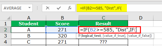
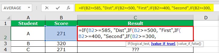
Now take a look at the popular nested IF example. We need to arrive at standards based on the student’s score. Consider the below data for an example.
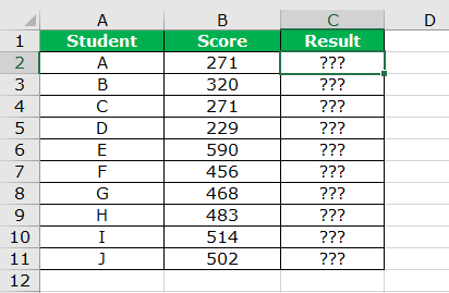
To arrive at the results, we need to test the below conditions. These conditions are nothing but our logical tests.
- If the score is >=585 result should be “Dist”
- If the score is >=500 result should be “First”
- If the score is >=400 result should be “Second”
- If the score is >=350 result should be “Pass”
- If all the above conditions are “FALSE,” the result should be “FAIL.”
Now, we have a total of 5 conditions to test. Unfortunately, the logical tests are more than one logical test at the moment. So we need to use Nested IFs to try multiple criteria.
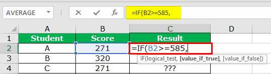
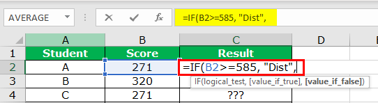
- We must open the IF condition and pass the first test, i.e., whether the score is >=585.

- If the above logical test is “TRUE,” we need the result as “Dist.” So, we must enter the result in double-quotes.

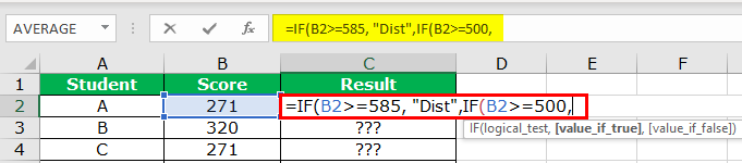
- The next argument is if the value or test is “FALSE.” If the test is “FALSE,” we have four more conditions to test, so we must open one more IF condition in Excel in the next argument.

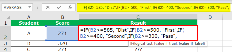
- Now, let us test the second condition here. The second condition is to test whether the score is >= 500. So, we must pass the argument as >=500.

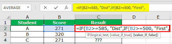
- If this test is true the result should be “First”. So, enter the result in double-quotes.

- We have already entered two excel IF conditions, if these two tests are FALSE then we need to test the third condition, so open one more IF now and pass the next condition i.e. test whether the score is 400 or not.

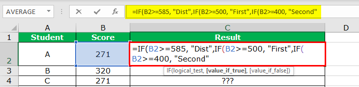
- If this test is “TRUE,” the result should be “Second.”

- Now the total number of IF conditions is 3. So, if all these IF conditions test is “FALSE,” we need one more condition to test, i.e., whether the score is >=300.

- If this condition is “TRUE,” the result is “Pass.”

- Now we came to the last argument. We have entered four IFs, so if all these conditions tests are “FALSE,” then the final result is “FAIL,” so enter “FAIL” as a result.

Like this, we can test multiple conditions by nesting many IF conditions inside the one IF condition.
The logic here is the first IF result will come if the logical test is “TRUE.” If the logical test is “FALSE,” then the second IF can be executed. Until the formula finds the “TRUE” test result, it will execute it. If none of the results is “TRUE,” it will execute the final “FALSE” result.


Example #2
Now take a look at the real-time corporate example of calculating sales commissionSales commission is a monetary reward awarded by companies to the sales reps who have managed to achieve their sales target. It is an incentive geared towards producing more sales and rewarding the performers while simultaneously recognizing their efforts. A sales commission agreement is signed to agree on the terms and conditions set for eligibility to earn a commission.read more. Consider the below data for the example.
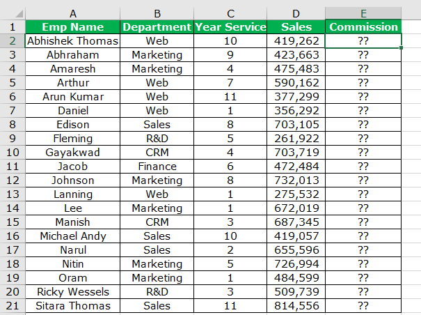
To arrive at the commission %, we need to test the below conditions.
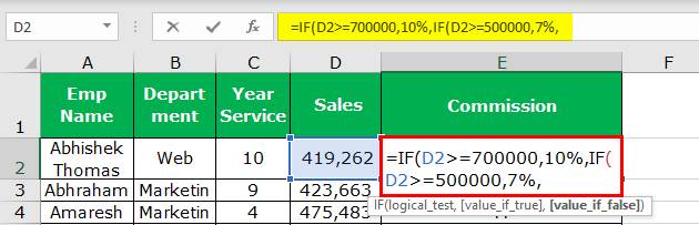
- If the sales value is >=7 lakhs, commission % is 10%.
- If the sales value is >=5 lakhs, commission % is 7%.
- If the sales value is >=4 lakhs, commission % is 5%.
- If the sales value is < 4 lakhs, the commission is 0%.
It is similar to the previous example. However, instead of arriving at results, we need to reach percentages. Let us apply the nested IF function in Excel.
- Step 1: We must first apply IF and test the first condition.
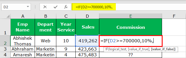
- Step 2: Then, we must use the second IF condition if the first test is “FALSE.”
- Step 3: If the above IF conditions are “FALSE,” test the third condition.
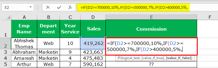
- Step 4: If all the above conditions are “FALSE, ” the result is 0%.
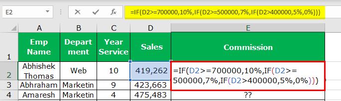
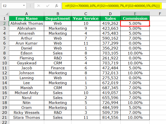
- Step 5: After that, we must copy the formula to the remaining cells. Consequently, it will provide us with the results.
Example #3
Take how to use other logical functions: AND with IF condition to test multiple conditions.
Take the same data from the above example. But we have slightly changed the data. We have removed the “Sales” column.
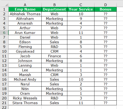
Here, we need to calculate a bonus for these employees based on the below conditions:
- If the employee’s department is “Marketing” and “Years of Service” is >5 years then the bonus is 50,000.
- If the employee’s department is “Sales” and “ Years of Service” is >5 years then the bonus is 45,000.
- If the service is > 5 years for all the other employees, the bonus is 25,000.
- If the year of service is <5 years, the bonus is zero.
It looks a bit completed.
To arrive at a single result, we need to test two conditions. When we need to test two conditions and if both the conditions should be “TRUE,” the AND logical condition can be used.
The Excel AND function will return the “TRUE” result if all the supplied conditions are “TRUE.” If one condition is “FALSE,” the result will be only “FALSE.”
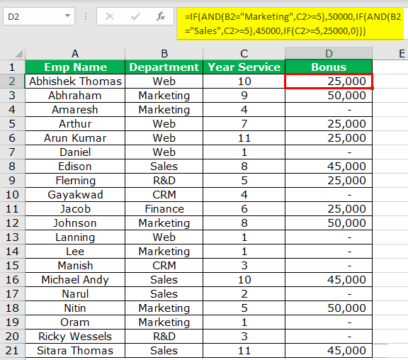
- Step 1: We must open the IF condition first.

- Step 2: Since we need to test two conditions to arrive at the result, let’s open AND function inside the IF condition.

- Step 3: Here, we need to test the conditions. The first condition is whether the department is “Marketing” or not, and the second condition is a “Years of Service” is >=5 years.

- Step 4: If the supplied conditions are “TRUE,” the bonus amount is 50000.

- Step 5: We must apply tests for the remaining conditions like this. We have already used the formula to arrive at the results.
Things to Remember
- The Excel AND function will return the “TRUE” result if all the supplied conditions are “TRUE.” If any of the conditions is “FALSE,” it will return “FALSE.”
- To arrive at the final result, we must apply one more rather. Then, we can pass the result in the “FALSE” argument only.
Recommended Articles
This article has been a guide to Nested IF Function in Excel. We discuss using the Nested IF function in Excel, practical examples, and a downloadable Excel template. You may learn more about Excel from the following articles: –
- Examples of Excel SUMIF Text
- Examples of Excel SUMIF Not Blank
- COUNTIF Function in Excel VBA
- SUMIF with Multiple Criteria in Excel
The IF function is one of the most heavily used functions in Excel. IF is a simple function, and people love IF because it gives them the power to make Excel respond as information is entered in a spreadsheet. With IF, you can bring your spreadsheet to life.
But one IF often leads to another, and once you combine more than a couple IFs, your formulas can start to look like little Frankensteins 
Are nested IFs evil? Are they sometimes necessary? What are the alternatives?
Read on to learn the answers to these questions and more…
1. Basic IF
Before we talk about nested IF, let’s quickly review the basic IF structure:
=IF(test,[true],[false])
The IF function runs a test and performs different actions depending on whether the result is true or false.
Note the square brackets…these mean the arguments are optional. However, you must supply either a value for true, or a value for false.
To illustrate, here we use IF to check scores and calculate «Pass» for scores of at least 65:

Cell D3 in the example contains this formula:
=IF(C3>=65,"Pass")
Which can be read like this: if the score in C3 is at least 65, return «Pass».
Note however that if the score is less than 65, IF returns FALSE, since we didn’t supply a value if false. To display «Fail» for non-passing scores, we can add «Fail» as the false argument like so:
=IF(C3>=65,"Pass","Fail")

Video: How to build logical formulas.
2. What nesting means
Nesting simply means to combine formulas, one inside the other, so that one formula handles the result of another. For example, here’s a formula where the TODAY function is nested inside the MONTH function:
=MONTH(TODAY())
The TODAY function returns the current date inside of the MONTH function. The MONTH function takes that date and returns the current month. Even moderately complex formulas use nesting frequently, so you’ll see nesting everywhere in more complex formulas.
3. A simple nested IF
A nested IF is just two more IF statements in a formula, where one IF statement appears inside the other.
To illustrate, below I’ve extended the original pass/fail formula above to handle «incomplete» results by adding an IF function, and nesting one IF inside the other:

=IF(C3="","Incomplete",IF(C3>=65,"Pass","Fail"))
The outer IF runs first and tests to see if C3 is blank. If so, outer IF returns «Incomplete», and the inner IF never runs.
If the score is not blank, the outer IF returns FALSE, and the original IF function is run.
4. A nested IF for scales
You’ll often see nested IFs set up to handle «scales»…for example, to assign grades, shipping costs, tax rates, or other values that vary on a scale with a numerical input. As long as there aren’t too many levels in the scale, nested IFs work fine here, but you must keep the formula organized, or it becomes difficult to read.
The trick is to decide a direction (high to low, or low to high), then structure the conditions accordingly. For example, to assign grades in a «low to high» order, we can represent the solution needed in the following table. Note there is no condition for «A», because once we’ve run through all the other conditions, we know the score must be greater than 95, and therefore an «A».
| Score | Grade | Condition |
| 0-63 | F | <64 |
| 64-72 | D | <73 |
| 73-84 | C | <85 |
| 85-94 | B | <95 |
| 95-100 | A |
With the conditions clearly understood, we can enter the first IF statement:
=IF(C5<64,"F")
This takes care of «F». Now, to handle «D», we need to add another condition:
=IF(C5<64,"F",IF(C5<73,"D"))
Note that I simply dropped another IF into the first IF for the «false» result. To extend the formula to handle «C», we repeat the process:
=IF(C5<64,"F",IF(C5<73,"D",IF(C5<85,"C")))
We continue on this way until we reach the last grade. Then, instead of adding another IF, just add the final grade for false.
=IF(C5<64,"F",IF(C5<73,"D",IF(C5<85,"C",IF(C5<95,"B","A"))))
Here is the final nested IF formula in action:

Video: How to make a nested IF to assign grades
5. Nested IFs have a logical flow
Many formulas are solved from the inside out, because «inner» functions or expressions must be solved first for the rest of the formula to continue.
Nested IFs have a their own logical flow, since the «outer» IFs act like a gateway to «inner» IFs. This means that results from outer IFs determine whether inner IFs even run. The diagram below visualized the logical flow of the grade formula above.

6. Use Evaluate to watch the logical flow
On Windows, you can use the Evaluate feature to watch Excel solve your formulas, step-by-step. This is a great way to «see» the logical flow of more complex formulas, and to troubleshoot when things aren’t working as you expect. The screen below shows the Evaluate window open and ready to go. Each time you click the Evaluate button, the «next step» in the formula is solved. You can find Evaluate on the Formulas tab of the ribbon (Alt M, V).

Unfortunately, the Mac version of Excel doesn’t contain the Evaluate feature, but you can still use the F9 trick below.
7. Use F9 to spot check results
When you select an expression in the formula bar and press the F9 key, Excel solves just the part selected. This is a powerful way to confirm what a formula is really doing . In the screen below, I am using the screen tip windows to select different parts of the formula, then clicking F9 to see that part solved:

Use Control + Z (Command + Z) on a Mac to undo F9. You can also press Esc to exit the formula editor without any changes.
Video: How to debug a formula with F9
8. Know your limits
Excel has limits on how deeply you can nest IF functions. Up to Excel 2007, Excel allowed up to 7 levels of nested IFs. In Excel 2007+, Excel allows up to 64 levels.
However, just because you can nest a lot of IFs, it doesn’t mean you should. Every additional level you add makes the formula more difficult to understand and troubleshoot. If you find yourself working with a nested IF more than a few levels deep, you should probably take a different approach — see the below for alternatives.
9. Match parentheses like a pro
One of the challenges with nested IFs is matching or «balancing» parentheses. When parentheses aren’t matched correctly, your formula is broken. Luckily, E xcel provides a couple tools to help you make sure parentheses are «balanced» while editing formulas.
First, once you have more than one set of parentheses, the parentheses are color-coded so that opening parentheses match closing parentheses. These colors are pretty darn hard to see, but they are there if you look closely:

Second (and better) when you close a parentheses, Excel will briefly bold the matching pair. You can also click into the formula and use the arrow key to move through parentheses, and Excel will briefly bold both parentheses when there is a matching pair. If there is no match, you’ll see no bolding.
Unfortunately, the bolding is a Windows-only feature. If you’re using Excel on a Mac to edit complex formulas, it sometimes makes sense to copy and paste the formula into a good text editor (Text Wrangler is free and excellent) to get better parentheses matching tools. Text Wrangler will flash when parentheses are matched, and you can use Command + B to select all text contained by parentheses. You can paste the formula back into Excel after you’ve straightened things out.
10. Use the screen tip window to navigate and select
When it comes to navigating and editing nested IFs, the function screen tip is your best friend. With it, you can navigate and precisely select all arguments in a nested IF:

You can see me use the screen tip window a lot in this video: How to build a nested IF.
11. Take care with text and numbers
Just as a quick reminder, when working with the IF function, take care that you a properly matching numbers and text. I often see formulas IF like this:
=IF(A1="100","Pass","Fail")
Is the test score in A1 really text and not a number? No? Then don’t use quotes around the number. Otherwise, the logical test will return FALSE even when the value is a passing score, because «100» is not the same as 100. If the test score is numeric, use this:
=IF(A1=100,"Pass","Fail")
12. Add line breaks make nested IFs easy to read
When you’re working with a formula that contains many levels of nested IFs, it can be tricky to keep things straight. Because Excel doesn’t care about «white space» in formulas (i.e. extra spaces or line breaks), you can greatly improve the readability of nested ifs by adding line breaks.
For example, the screen below shows a nested IF that calculates a commission rate based on a sales number. Here you can see the typical nested IF structure, which is hard to decipher:

However, if I add line breaks before each «value if false», the logic of the formula jumps out clearly. Plus, the formula is easier to edit:

You can add line breaks on Windows with Alt + Enter, on a Mac, use Control + Option + Return.
Video: How to make a nested IF easier to read.
13. Limit IFs with AND and OR
Nested IFs are powerful, but they become complicated quickly as you add more levels. One way to avoid more levels is to use IF in combination with the AND and OR functions. These functions return a simple TRUE/FALSE result that works perfectly inside IF, so you can use them to extend the logic of a single IF.
For example, in the problem below, we want to put an «x» in column D to mark rows where the color is «red» and the size is «small».

We could write the formula with two nested IFs like this:
=IF(B6="red",IF(C6="small","x",""),"")
However, by replacing the test with the AND function, we can simplify the formula:
=IF(AND(B6="red",C6="small"),"x","")
In the same way, we can easily extend this formula with the OR function to check for red OR blue AND small:
=IF(AND(OR(B4="red",B4="blue"),C4="small"),"x","")
All of this could be done with nested IFs, but the formula would rapidly become more complex.
Video: IF this OR that
14. Replace Nested IFs with VLOOKUP
When a nested IF is simply assigning values based on a single input, it can be easily replaced with the VLOOKUP function. For example, this nested IF assigns numbers to five different colors:
=IF(E3="red",100,IF(E3="blue",200,IF(E3="green",300,IF(E3="orange",400,500))))
We can easily replace it with this (much simpler) VLOOKUP:
=VLOOKUP(E3,B3:C7,2,0)

As a bonus, VLOOKUP keeps values on the worksheet (where they can be easily changed) instead of embedding them in the formula.
Although the formula above uses exact matching, you can easily use VLOOKUP for grades as well.
See also: 23 things to know about VLOOKUP
Video: How to use VLOOKUP
Video: Why VLOOKUP is better than nested IFs
15. Choose CHOOSE
The CHOOSE function can provide an elegant solution when you need to map simple, consecutive numbers (1,2,3, etc.) to arbitrary values.
In the example below, CHOOSE is used to create custom weekday abbreviations:

Sure, you could use a long and complicated nested IF to do the same thing, but please don’t
16. Use IFS instead of nested IFs
If you’re using Excel 2016 via Office 365, there’s a new function you can use instead of nested IFs: the IFS function. The IFS function provides a special structure for evaluating multiple conditions without nesting:

The formula used above looks like this:
=IFS(D5<60,"F",D5<70,"D",D5<80,"C",D5<90,"B",D5>=90,"A")
Note we have just a single pair of parentheses!
What happens when you open a spreadsheet that uses the IFS function in an older version of Excel? In Excel 2013 and 2010 (and I believe Excel 2007, but can’t test) you’ll see «_xlfn.» appended to the IFS in the cell. The previously calculated value will still be there, but if something causes the formula to recalculate, you’ll see a #NAME error. Microsoft has more information here.
17. Max out
Sometimes, you can use MAX or MIN in a very clever way that avoids an IF statement. For example, suppose you have a calculation that needs to result in a positive number, or zero. In other words, if the calculation returns a negative number, you just want to show zero.
The MAX function gives you a clever way to do this without an IF anywhere in sight:
=MAX(calculation,0)
This technique returns the result of the calculation if positive, and zero otherwise.
I love this construction because its just so simple. See this article for a full write-up.
18. Trap errors with IFERROR
A classic use of IF is to trap errors and supply another result when an error is thrown, like this:
=IF(ISERROR(formula),error_result,formula)
This is ugly and redundant, since same formula goes in twice, and Excel has to calculate the same result twice when there is no error.
In Excel 2007, the IFERROR function was introduced, which lets you trap errors much more elegantly:
=IFERROR(formula,error_result)
Now when the formula throws an error, IFERROR simply returns the value you provide.
19. Use boolean logic
You can also sometimes avoid nested IFs by using what’s called «boolean logic». The word boolean refers to TRUE/FALSE values. Although Excel displays the words TRUE and FALSE in cells, internally, Excel treats TRUE as 1, and FALSE as zero. You can use this fact to write clever, and very fast formulas. For example, in the VLOOKUP example above, we have a nested IF formula that looks like this:
=IF(E3="red",100,IF(E3="blue",200,IF(E3="green",300,IF(E3="orange",400,500))))
Using boolean logic, you can rewrite the formula like this:
=(E3="red")*100+(E3="blue")*200+(E3="green")*300+(E3="orange")*400+(E3="purple")*500
Each expression performs a test, and then multiples the outcome of the test by the «value if true». Since tests return either TRUE or FALSE (1 or 0), the FALSE results effectively cancel themselves out the formula.
For numeric results, boolean logic is simple and extremely fast, since there is no branching. On the downside, boolean logic can be be confusing to people who aren’t used to seeing it. Still, it’s a great technique to know about.
Video: How to use boolean logic in Excel formulas
When do you need a nested IF?
With all these options for avoiding nested IFs, you might wonder when it makes sense to use a nested IF?
I think nested IFs make sense when you need to evaluate several different inputs to make a decision.
For example, suppose you want to calculate an invoice status of «Paid», «Open», «Overdue», etc. This requires that you look at the invoice age and outstanding balance:

In this case, a nested IF is a perfectly fine solution.
Your thoughts?
What about you? Are you an IF-ster? Do you avoid nested IFs? Are nested IFs evil? Share your thoughts below.
Things will not always be the way we want them to be. The unexpected can happen. For example, let’s say you have to divide numbers. Trying to divide any number by zero (0) gives an error. Logical functions come in handy such cases. In this tutorial, we are going to cover the following topics.
In this tutorial, we are going to cover the following topics.
- What is a Logical Function?
- IF function example
- Excel Logic functions explained
- Nested IF functions
What is a Logical Function?
It is a feature that allows us to introduce decision-making when executing formulas and functions. Functions are used to;
- Check if a condition is true or false
- Combine multiple conditions together
What is a condition and why does it matter?
A condition is an expression that either evaluates to true or false. The expression could be a function that determines if the value entered in a cell is of numeric or text data type, if a value is greater than, equal to or less than a specified value, etc.
IF Function example
We will work with the home supplies budget from this tutorial. We will use the IF function to determine if an item is expensive or not. We will assume that items with a value greater than 6,000 are expensive. Those that are less than 6,000 are less expensive. The following image shows us the dataset that we will work with.
 and conditions in Excel")
- Put the cursor focus in cell F4
- Enter the following formula that uses the IF function
=IF(E4<6000,”Yes”,”No”)
HERE,
- “=IF(…)” calls the IF functions
- “E4<6000” is the condition that the IF function evaluates. It checks the value of cell address E4 (subtotal) is less than 6,000
- “Yes” this is the value that the function will display if the value of E4 is less than 6,000
-
“No” this is the value that the function will display if the value of E4 is greater than 6,000
When you are done press the enter key
You will get the following results
 and conditions in Excel")
Excel Logic functions explained
The following table shows all of the logical functions in Excel
| S/N | FUNCTION | CATEGORY | DESCRIPTION | USAGE |
|---|---|---|---|---|
| 01 | AND | Logical | Checks multiple conditions and returns true if they all the conditions evaluate to true. | =AND(1 > 0,ISNUMBER(1)) The above function returns TRUE because both Condition is True. |
| 02 | FALSE | Logical | Returns the logical value FALSE. It is used to compare the results of a condition or function that either returns true or false | FALSE() |
| 03 | IF | Logical |
Verifies whether a condition is met or not. If the condition is met, it returns true. If the condition is not met, it returns false. =IF(logical_test,[value_if_true],[value_if_false]) |
=IF(ISNUMBER(22),”Yes”, “No”) 22 is Number so that it return Yes. |
| 04 | IFERROR | Logical | Returns the expression value if no error occurs. If an error occurs, it returns the error value | =IFERROR(5/0,”Divide by zero error”) |
| 05 | IFNA | Logical | Returns value if #N/A error does not occur. If #N/A error occurs, it returns NA value. #N/A error means a value if not available to a formula or function. |
=IFNA(D6*E6,0) N.B the above formula returns zero if both or either D6 or E6 is/are empty |
| 06 | NOT | Logical | Returns true if the condition is false and returns false if condition is true |
=NOT(ISTEXT(0)) N.B. the above function returns true. This is because ISTEXT(0) returns false and NOT function converts false to TRUE |
| 07 | OR | Logical | Used when evaluating multiple conditions. Returns true if any or all of the conditions are true. Returns false if all of the conditions are false |
=OR(D8=”admin”,E8=”cashier”) N.B. the above function returns true if either or both D8 and E8 admin or cashier |
| 08 | TRUE | Logical | Returns the logical value TRUE. It is used to compare the results of a condition or function that either returns true or false | TRUE() |
A nested IF function is an IF function within another IF function. Nested if statements come in handy when we have to work with more than two conditions. Let’s say we want to develop a simple program that checks the day of the week. If the day is Saturday we want to display “party well”, if it’s Sunday we want to display “time to rest”, and if it’s any day from Monday to Friday we want to display, remember to complete your to do list.
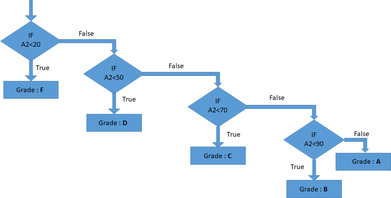
A nested if function can help us to implement the above example. The following flowchart shows how the nested IF function will be implemented.
 and conditions in Excel")
The formula for the above flowchart is as follows
=IF(B1=”Sunday”,”time to rest”,IF(B1=”Saturday”,”party well”,”to do list”))
HERE,
- “=IF(….)” is the main if function
- “=IF(…,IF(….))” the second IF function is the nested one. It provides further evaluation if the main IF function returned false.
Practical example
 and conditions in Excel")
Create a new workbook and enter the data as shown below
 and conditions in Excel")
- Enter the following formula
=IF(B1=”Sunday”,”time to rest”,IF(B1=”Saturday”,”party well”,”to do list”))
- Enter Saturday in cell address B1
- You will get the following results
 and conditions in Excel")
Download the Excel file used in Tutorial
Summary
Logical functions are used to introduce decision-making when evaluating formulas and functions in Excel.
In our last post, we talked about the IF Statement, which is one of the most important functions in Excel. The limitation of the IF statement is that it has only two outcomes. But if you are dealing with multiple conditions then Excel Nested If’s can come in very handy.
Nested if’s are the formulas that are formed by multiple if statements one inside another. This nesting makes it possible for a single formula to take multiple decisions. In Excel 2003 nesting was only possible up to 7 levels but Excel 2007 has increased this number to 64.
Syntax of Excel Nested IF formula:
The syntax of the nested IF statement is as follows:
=IF(Condition_1,Value_if_True_1,IF(Condition_2,Value_if_True_2,Value_if_False_2))
Here, ‘Condition_1’ refers to the condition used in the first IF.‘Value_if_True_1’ will be the result if the first IF statement is True.‘Condition_2’ is the condition used in the second IF. The second IF will only come into picture when the First IF statement results a False value.‘Value_if_True_2’ will be the result if the second IF statement is True.‘Value_if_False_2’ will be the result if the second IF statement is False.
This is equivalent to:
IF Condition1 = true THEN value_if_true1 'If Condition1 is true
ELSE IF Condition2 = true THEN value_if_true2 'If Condition2 is true
ELSE value_if_false2 'If both conditions are false
END IF 'End of IF Statement
Example of Nested IF’s in Excel:
Now, let’s understand Nested If’s with an example.
Example 1:
In the below image an Employee table of a company is shown. The company decides to give a bonus to its employees but their bonus criteria is quite strange. As you can see in the below image they are giving 20% bonus to the North Region Employees, 30% to the South Region Employees, 40% to the East Region Employees and 50% to the West Region Employees.

In this case, we can use Excel Nested IF formula to find the bonus for each employee. The formula can be:
=IF(B2="North","20%",IF(B2="South","30%",IF(B2="East","40%",IF(B2="West","50%", "Region is Invalid"))))
The formula is quite simple, it just checks if ‘B2’ (the cell that contains region details for the first employee) is equal to “North”, then the value should be 20%, if not then check if B2 is equal to “South”, if yes then the value should be 30%, if not move on to next IF statement and so on.
Similarly, for the second employee the formula would be:
=IF(B3="North","20%",IF(B3="South","30%",IF(B3="East","40%",IF(B3="West","50%", "Region is Invalid"))))
In this case, I have handled another important thing i.e. If the Region does not match with any one of the IF conditions then the output should be “Region is Invalid”.
Example 2:
In the second example, we have a table of students and their scores. Now based on their scores we have to give a grade to the students.

Students with scores below 40 are considered as “Fail”, scores between 41 and 60 are considered “Grade C”, scores between 61 and 75 are considered “Grade B” and scores between 76 and 100 are considered as “Grade A”
In this scenario, we can use a nested If formula as:
=IF(B2<=40,"Fail",IF(AND(B2>=41,B2<=60),"Grade C",IF(AND(B2>=61,B2<=75),"Grade B",IF(AND(B2>=76,B2<=100),"Grade A"))))
This formula just checks if B2 (cell containing the score of the first student) is less than or equal to 40, if true then the value should be “Fail” if not then check the next IF condition and so on.
You can see that here in the inner-most IF statement I haven’t used the ‘Value_if_False’, it is perfectly alright to omit this parameter in such a case. In-case all the IF conditions in this formula will result in a False value then the formula will simply return a ‘FALSE’ keyword.
So, this was all about Nested IF Instruction. Feel free to drop your comments related to the topic.
Excel Nested IF Formula (Table of Contents)
- Nested IF Formula in Excel
- How to Use Nested IF Formula in Excel?
Nested IF Formula in Excel
IF Function is one of the most commonly & frequently used logical function in Excel.
Usually, IF function runs a logical test & checks whether a condition or criteria is met or not, and returns one value in a result, it may be either, if true and another value if false, these are the two possible outcomes with if function.
Sometimes you need to work with situations or conditions where there are more than two possible outcomes; in this scenario, the Nested IF Formula helps you out.
Nesting means a combination of formulas, one inside the other, where each formula controls or handles the result of others.
![]()
Nested IF Formula is categorized under Advanced IF functions which allow you to check more than one condition.
From excel 2007 version onwards, 64 IF statements or functions can be used in one formula (In Nested IF Formula)
Nested IF Formula: It’s an If function within an if function to test multiple conditions.
Syntax of Nested IF Formula:
=IF(condition, value_if_true1, IF(second condition, value_if_true2, value_if_false2 ))
The Nested IF Formula syntax or formula has the below-mentioned arguments:
- Condition: It is the value that you want to test.
- value_if_true: The value appears or returns if the logical condition evaluates to TRUE.
- value_if_false: The value appears or returns if the logical condition evaluates to FALSE.
Various arithmetic operators that can be used in the Nested IF Formula:
> Greater Than
= Equal to
< Less Than
>= Greater than or equal to
<= Less than or equal to
<> Less than or greater than
These above-mentioned operators are used in the Criteria or Condition argument of Nested IF Formula’s statement; it is purely based on a logic that you apply in the criteria argument.
How to Use NESTED IF Formula in Excel?
Let’s check out how this formula Formula works in Excel
You can download this Nested IF Formula Excel Template here – Nested IF Formula Excel Template
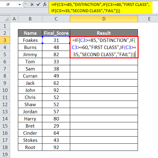
Example #1
Let us analyze the Nested IF Formula with Multiple Criteria.
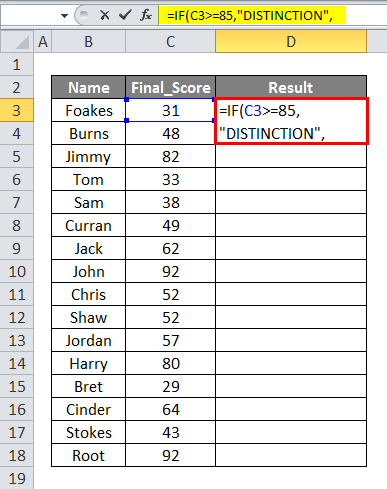
In the below-mentioned example, the table contains a list of the student in column B (B2 to B18) & the score of each student (C2 to C18).
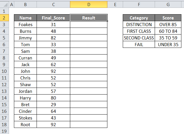
Here, I want to categorize their scores with the below-mentioned conditions:
DISTINCTION: Over 85.
FIRST CLASS: Between 60 and 84, inclusive.
SECOND CLASS: Between 35 and 59, inclusive.
FAIL: Under 35.
With the above conditions, I need to categorize students’ results based on their score, Here Nested IF Formula. I need to build that formula with multiple IF statements.
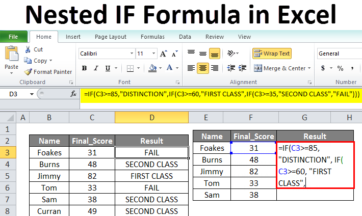
Let’s start entering the first IF statement:
=IF(C3>85,”DISTINCTION”,
This takes care of the “DISTINCTION” category students now if I want to handle the second category. “FIRST CLASS”, I need to add another conditional statement:
=IF(C3>=85,”DISTINCTION”, IF(C3>=60, “FIRST CLASS”,
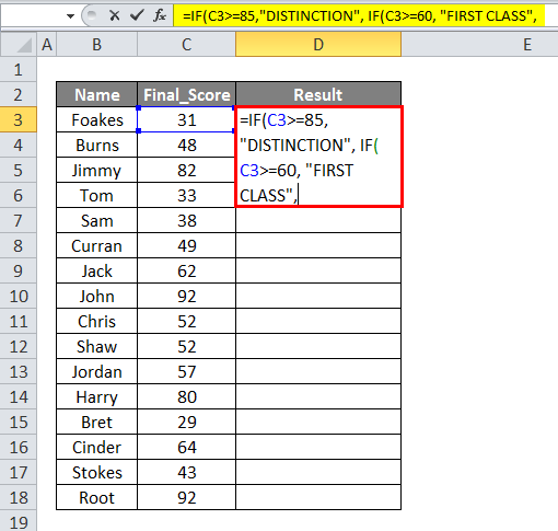
Note: In the above-mentioned syntax, I simply added another IF statement into the first IF statement. Similarly, I extend the formula to handle the next category, “SECOND CLASS”, where I repeat the above-mentioned step once again.
=IF(C3>=85,”DISTINCTION”, IF(C3>=60, “FIRST CLASS”, IF(C3>=35, “SECOND CLASS”,
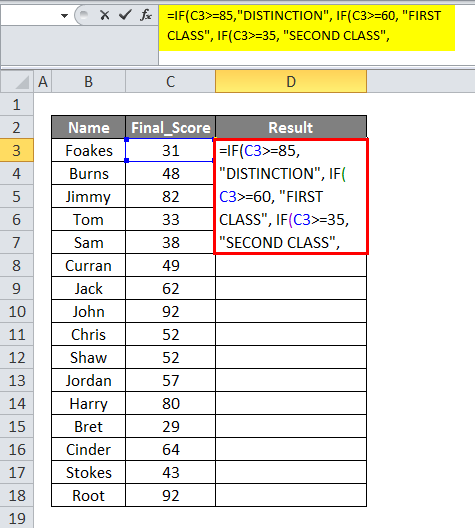
I continue with similar steps until I reach the last category. Now, I have left with the last category, “FAIL”, if the last category or criteria appears, instead of adding another IF, just I need to add the “FAIL” for a false argument (value_if_false argument).
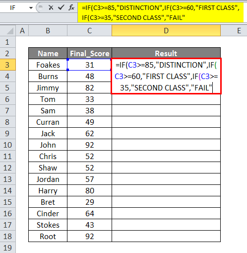
After entering the last category, you need to close it with three closed brackets.
In the last criteria, value_if_false argument, if the score is less than 35, IF function returns FALSE, as we don’t supply a value if false.
=IF(C3>=85,”DISTINCTION”,IF(C3>=60,”FIRST CLASS”,IF(C3>=35,”SECOND CLASS”,”FAIL”)))
Now, The Nested IF Formula is ready; copy this formula in the cell “D3” and click on enter to get the result. Simultaneously this formula is applied to the whole range by selecting a cell from “D3” to “D18” and click on CTRL + D to get the result.
How Excel Nested IF Logical Test Works?
=IF(C3>=85,”DISTINCTION”,IF(C3>=60,”FIRST CLASS”,IF(C3>=35,”SECOND CLASS”,”FAIL”)))
Now let’s split or break-up the above formula and check out.
=IF(C3>=85,”DISTINCTION”,
IF(C3>=60,”FIRST CLASS”,
IF(C3>=35,”SECOND CLASS”,”FAIL”)))
Or
IF(check if C3>=85, if true – return “DISTINCTION”, or else
IF(check if C3>=60, if true – return “FIRST CLASS”, or else
IF(check if C3>=35, if true – return “SECOND CLASS”, if false –
return “FAIL”)))
Here, the Nested IF formula actually directs the excel to evaluate the logical test for the first IF function; in the result, if the condition or criteria is met, then it returns the supplied value (“DISTINCTION”) in the value_if_true argument. Otherwise or else, If the condition or criteria of the first If a function is not met, then go ahead and carry out or test the second If statement and follow the similar step until the last criteria.
Conclusion
In the below-mentioned screenshot, you can observe, usually, parenthesis pairs are shaded in various or different colors so that the opening parenthesis matches the closing one at the end.
![]()
- Text values should always be enclosed in double-quotes “DISTINCTION.”
Note: Never present the numbers or numeric values in the double quotes, e.g. 85, 60 & 35
![]()
- You can add line break or spaces in the formula bar to understand this Formula in a better & easier way.
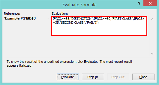
- Evaluate Formula feature is located on the Formula tab under the Formula Auditing group or subsection. This feature helps out to solve your complex formula. Nested IF Formula step by step.
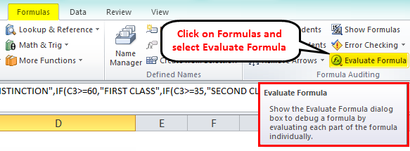
When you click on the evaluate button frequently, it will show you all the evaluation process steps (From beginning to end, how the formula works step by step process).
Things to Remember
- When using the Nested IF Formula, we should not start the second criteria in the IF function with the = sign.
- Apart from arithmetic operators, you can also use addition, subtraction, multiplication & division symbols, e.g. =IF(C1<10, C1*4,
- The order of IF statements in the Nested IF Formula is very important to evaluate the logical test. If the IF function’s first condition evaluates TRUE, then subsequent conditions or IF statements don’t work. The formula stops at first result TRUE.
- Parenthesis Match: It is an important Criteria in the Nested IF formula; if the parentheses do not match, then the Nested IF formula won’t work.
Recommended Articles
This has been a guide to Nested IF Formula in Excel. Here we discuss How to use the Nested IF Formula in Excel along with practical examples and a downloadable excel template. You can also go through our other suggested articles-
- COUNTIF Formula in Excel
- COUNTIF Excel Function
- Excel IF Function
- Excel IF AND Function
In this tutorial, we will learn about the IF function in Excel. Along with IF, the AND and OR functions are important formulas too. A nested IF simply means multiple IF functions in a single syntax.
Introducing IF Function in Excel
Let’s get started with this easy guide to using the IF function and all its related functions in Microsoft Excel, step-by-step with supporting images and examples.
1. IF Function
To learn to use the IF function, we will take an example of a mark list of students below.

Our goal is to find out which student has passed or failed and what are their grades. Of course, it would be a tedious task to find out pass or fail results and grades for each student in this list.
To ease our task, we have IF functions for that matter. The IF function will automatically identify if a student has passed or failed based on the criteria you provide to it.
It will automatically mark a student as “Pass” if he/she has scored above the minimum pass mark and mark a student as “Fail” if he/she has scored below the minimum pass mark.
The IF function automatically assigns the appropriate grades to students based on their marks if you command it.
Here is a glimpse of how the IF function helps you out with assigning grades and marking “Pass” or “Fail”.

Steps to use IF function in Excel
We have allotted certain grades and marked them as Pass or Fail to students based on the percentages they have secured in their exams, with the help of the IF function.
1. Using the IF function in Excel to identify passed/failed students
Let’s learn how we can use the IF formula to achieve this. We will use the same example. We take the minimum passing percentage as 34%.

- Find out the percentage of total marks of every student.
- Create a new column named “Pass/Fail”.
- In the blank cell below the title, type the IF formula as follows next.
- Type =IF( and select the first student’s percentage and type >=34.
- Put a comma and move to the next argument named [value_if_true]. This means you’re being asked to put a value to be displayed if the above condition is true. Remember these arguments are case sensitive.
- Once you have put a comma, type “Pass”.
- Put a comma and move to the next argument named [value_if_false] to display a value when the above condition is false. This field is optional in most cases but we need a false value because it is a mark list.
- Close the bracket and hit ENTER.

You can see that the formula is displaying “Pass” for the first student because she has secured above 34%.
- Double-click or drag the cell from the right corner below to autofill the formula to all the students below.

Recommended read: How to Autofill in Excel?
2. Nested IF Function
Now, let us start assigning grades to all students.
We are going to be using multiple IF functions in a single syntax this time to provide multiple criteria to the IF function. This is called Nested IF in Excel.
However, there is no specific function named “Nested IF” in Excel, it is simply that this behavior has been given a name i.e., Nested IF.
Before we proceed further, we need to first make a table that displays a grading class for each grade. Here is an example below.

- Create a new column named “Grade”.
- Type the IF function in a blank cell below the title as follows.
- Type =IF( and now type AE118>=85,”A”,IF(AE118>=70,”B”,IF(AE118>=55,”C”,IF(AE118>=34,”D”,IF(AE118<=33,”Fail”.

- Note that AE118 is our cell address for the first student’s percentage. It will be different in your case. Refer to the image above to make sense of the formula.
- The formula simply states- if percentage marks are above and equal to 85 then give “A”, if percentage marks are above and equal to 70 then give “B”, and so on and so forth. For the last condition, we have applied the condition- if the marks are less than or equal to 33 then give “Fail”.
- For the last IF statement, you can either put the result as “Fail” or “E” as you like.
- Now, note that we will close the formula with 5 brackets for this example as we have used a total of 5 IF formulas.

- Hit ENTER to complete the formula.

You can now see that the formula has been applied to the first entry and the result is B because the student has secured 72.5% which is less than 75%. This means the nested Ifs are working correctly.
- Now drag the cell from the lower right corner to autofill the formula to the rest of the entries.

You can see that we now have grades and pass/fail markings for every student on the list successfully.
3. IF with AND in Excel
Let us learn the IF formula with the AND function in a single syntax with a minor example.

When you have two or more distinct conditions to be used together, you can use the IF function with AND in Excel.
While nested IFs will also work, using AND function will save your time as it is shorter to type. So, let’s get started.
Our goal is to identify currencies with revenues greater than 20,000 and less than 50,000 and mark them as “Good”.
- Type =IF(AND( because we are using the IF with AND function.
- Select the first cell under Revenue, and type >20000.
- Put a comma and select the first cell under Revenue again and type <50000.
- Now, close the bracket to complete the AND function. We’re still working on the IF function so do not put two brackets.
- We come back to the IF function as soon as we close the AND function. Now put the values to be displayed if the condition is true or false.
- Put a comma to move to the argument [value_if_true] and type “Good”.
- You can provide a result in the [value_if_false] argument, but it is completely optional. If nothing is provided then the cells will display FALSE if the condition is false. But if you want the cells to remain blank simply put “” (two double quotation marks) in this argument.
- Close the bracket to complete the IF function as well.

This is how the syntax should look like before pressing ENTER.
- Hit ENTER to view results and drag the cell down to autofill the formula to the rest of the cells.

There are only two such cells for which the condition is true and the result is being displayed as “Good” for them and the rest of the cells are blank. This means the formula is working correctly.
4. IF with OR in Excel
Using the OR function with the IF function will give results for either of the conditions that are true.
- Type =IF(OR(.
- Select the first cell under Revenue and type >=20000.
- Put a comma and select the first cell under Revenue again and type <=50000.
- Now, close the bracket to complete the OR function. We’re still working on the IF function so do not put two brackets.
- Coming back to the IF function, we now put the values to be displayed if the condition is true or false.
- Put a comma to move to the argument [value_if_true] and type “Flag”.
- Put a comma to move to the argument [value_if_false] and type “”.

This is how the syntax should look like before pressing ENTER.
- Close the bracket to complete the OR function and hit ENTER.
- Drag the cell below to get the results for the rest.

The formula is true for all entries and so it is displaying “Flag” for all of them. This is because all the values are either lower than 50,000 or greater than 20,000.
Conclusion
This was all about IF functions and other related functions to the IF function that are AND and OR functions.
Reference: ExcelJet
In this article, we will learn How to use nested IF formulas in Excel.
What are nested formulas in Excel ?
Nest means a pile of things built of multiple single things. When you start doing excel you will not evaluate the result using one function at a time. You use multiple functions in one formula. This is done to save space and time and is usual practice. Let’s learn nested formula syntax and illustrate an example to understand better.
nested IF formula Function in Excel
IF function is used for logic_test and returns value on the basis of the result of the logic_test.
Formula Syntax:
=IF(first_condition ,value_if_first_true, IF(second_condition, value_if_second_true, third_condition, value_if_third_true, value_if_none_is_true)
Nested IF is an iteration of IF function. It runs multiple logic_test in one formula. IFS function is built in function use instead for nested IF function in version above Excel 2016..
Example :
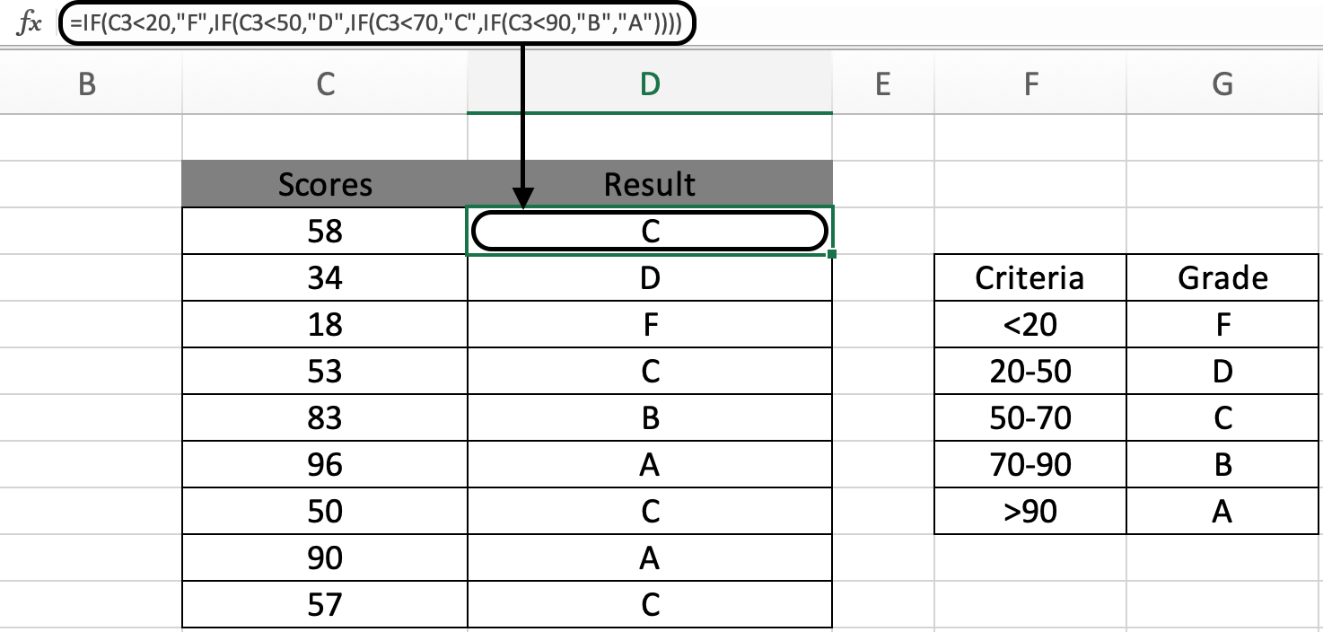
All of these might be confusing to understand. Let’s understand how to use the function using an example. Here we gave a list of student scored marks on a test. As a teacher you need to update the grade column evaluating the scores criteria.
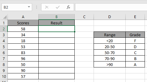
We will use the below process. Let’s understand.
Use the formula:
=IF(C3 < 20,»F»,IF(C3 < 50,»D»,IF(C3 < 70,»C»,IF(C3 < 90,»B»,»A»))))
C3<20 : test1
“F”: return F if test1 satisfies.
C3<50: test2
“D”: return D if test2 satisfies.
C3<90: test3
”B”: return B if test3 satisfies.
C3>90: test4
“A”: return A if test3 satisfies.

Applying the formula in other cells using CTRL + D.
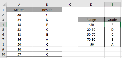
As you can see it’s easy to get the Grades having multiple conditions.
IF — AND Function in Excel
Here We have a list of Scores and We need to know under which criteria it lies.
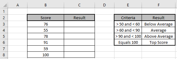
Here multiple criterias are needed to satisfy. Use the formula to match the given criteria table
Formula:
=IF(AND(B3 > 50, B3 < 60), «Below Average»,IF(AND(B3 > 60, B3 < 90),»Average»,IF(AND(B3 > 90,B3< 100),»Above Average»,»Top Score»)))
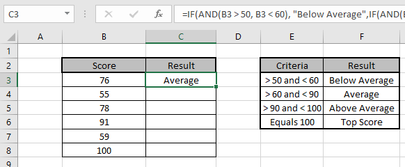
Copy the formula in other cells, select the cells taking the first cell where the formula is already applied, use shortcut key Ctrl + D
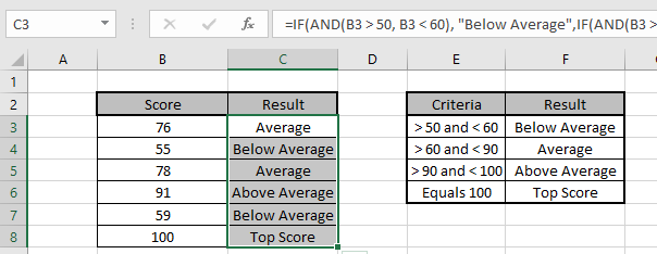
We got the Results corresponding to the Scores.
You can use IF and AND function to meet multiple conditions in a single formula.
Here are all the observational notes using the nested IF formula in Excel
Notes :
- Use the IFS function in the latest version of excel (after Excel 2017).
- Logic Operators like equals to ( = ), less than equal to ( <= ), greater than ( > ) or not equals to ( <> ) can be performed within a function applied with number only.
- Mathematical operators like SUM ( + ), Subtract ( — ), product ( * ), division ( / ), percent ( % ), power ( ^ ) can be performed over numbers using the example.
Hope this article about How to use nested IF formulas in Excel is explanatory. Find more articles on calculating values and related Excel formulas here. If you liked our blogs, share it with your friends on Facebook. And also you can follow us on Twitter and Facebook. We would love to hear from you, do let us know how we can improve, complement or innovate our work and make it better for you. Write to us at info@exceltip.com.
Related Articles :
IF with AND function : Implementation of logic IF function with AND function to extract results having criteria in Excel.
IF with OR function : Implementation of logic IF function with OR function to extract results having criteria in excel data.
How to use the IFS function : nested IF function operates on data having multiple criteria. The use of repeated IF function is nested IF excel formula.
SUMIFS using AND-OR logic : Get the sum of numbers having multiple criteria applied using logic AND-OR excel function.
Minimum value using IF function : Get the minimum value using the excel IF function and MIN function on array data.
How to use wildcards in excel : Count cells matching phrases using the wildcards in excel
Popular Articles :
How to use the IF Function in Excel : The IF statement in Excel checks the condition and returns a specific value if the condition is TRUE or returns another specific value if FALSE.
How to use the VLOOKUP Function in Excel : This is one of the most used and popular functions of excel that is used to lookup value from different ranges and sheets.
How to use the SUMIF Function in Excel : This is another dashboard essential function. This helps you sum up values on specific conditions.
How to use the COUNTIF Function in Excel : Count values with conditions using this amazing function. You don’t need to filter your data to count specific values. Countif function is essential to prepare your dashboard.