
What’s in the name?
If you are working with Excel spreadsheets, it could mean a lot of time saving and efficiency.
In this tutorial, you’ll learn how to create Named Ranges in Excel and how to use it to save time.
Named Ranges in Excel – An Introduction
If someone has to call me or refer to me, they will use my name (instead of saying a male is staying in so and so place with so and so height and weight).
Right?
Similarly, in Excel, you can give a name to a cell or a range of cells.
Now, instead of using the cell reference (such as A1 or A1:A10), you can simply use the name that you assigned to it.
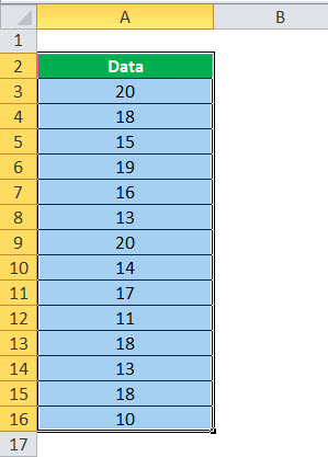
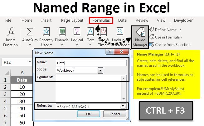
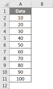
For example, suppose you have a data set as shown below:
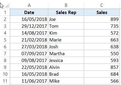
In this data set, if you have to refer to the range that has the Date, you will have to use A2:A11 in formulas. Similarly, for Sales Rep and Sales, you will have to use B2:B11 and C2:C11.
While it’s alright when you only have a couple of data points, but in case you huge complex data sets, using cell references to refer to data could be time-consuming.
Excel Named Ranges makes it easy to refer to data sets in Excel.
You can create a named range in Excel for each data category, and then use that name instead of the cell references. For example, dates can be named ‘Date’, Sales Rep data can be named ‘SalesRep’ and sales data can be named ‘Sales’.

You can also create a name for a single cell. For example, if you have the sales commission percentage in a cell, you can name that cell as ‘Commission’.
Benefits of Creating Named Ranges in Excel
Here are the benefits of using named ranges in Excel.
Use Names instead of Cell References
When you create Named Ranges in Excel, you can use these names instead of the cell references.
For example, you can use =SUM(SALES) instead of =SUM(C2:C11) for the above data set.
Have a look at ṭhe formulas listed below. Instead of using cell references, I have used the Named Ranges.
- Number of sales with value more than 500: =COUNTIF(Sales,”>500″)
- Sum of all the sales done by Tom: =SUMIF(SalesRep,”Tom”,Sales)
- Commission earned by Joe (sales by Joe multiplied by commission percentage):
=SUMIF(SalesRep,”Joe”,Sales)*Commission
You would agree that these formulas are easy to create and easy to understand (especially when you share it with someone else or revisit it yourself.
No Need to Go Back to the Dataset to Select Cells
Another significant benefit of using Named Ranges in Excel is that you don’t need to go back and select the cell ranges.
You can just type a couple of alphabets of that named range and Excel will show the matching named ranges (as shown below):

Named Ranges Make Formulas Dynamic
By using Named Ranges in Excel, you can make Excel formulas dynamic.
For example, in the case of sales commission, instead of using the value 2.5%, you can use the Named Range.
Now, if your company later decides to increase the commission to 3%, you can simply update the Named Range, and all the calculation would automatically update to reflect the new commission.
How to Create Named Ranges in Excel
Here are three ways to create Named Ranges in Excel:
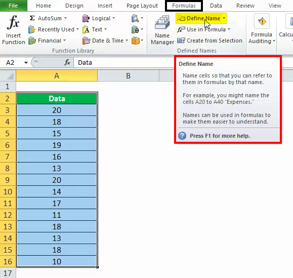
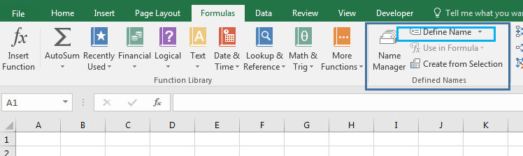
Method #1 – Using Define Name
Here are the steps to create Named Ranges in Excel using Define Name:
This will create a Named Range SALESREP.
Method #2: Using the Name Box
- Select the range for which you want to create a name (do not select headers).
- Go to the Name Box on the left of Formula bar and Type the name of the with which you want to create the Named Range.

- Note that the Name created here will be available for the entire Workbook. If you wish to restrict it to a worksheet, use Method 1.
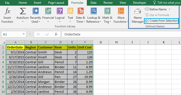
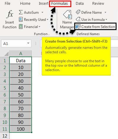
Method #3: Using Create From Selection Option
This is the recommended way when you have data in tabular form, and you want to create named range for each column/row.
For example, in the dataset below, if you want to quickly create three named ranges (Date, Sales_Rep, and Sales), then you can use the method shown below.
Here are the steps to quickly create named ranges from a dataset:
This will create three Named Ranges – Date, Sales_Rep, and Sales.
Note that it automatically picks up names from the headers. If there are any space between words, it inserts an underscore (as you can’t have spaces in named ranges).
Naming Convention for Named Ranges in Excel
There are certain naming rules you need to know while creating Named Ranges in Excel:
- The first character of a Named Range should be a letter and underscore character(_), or a backslash(). If it’s anything else, it will show an error. The remaining characters can be letters, numbers, special characters, period, or underscore.
- You can not use names that also represent cell references in Excel. For example, you can’t use AB1 as it is also a cell reference.
- You can’t use spaces while creating named ranges. For example, you can’t have Sales Rep as a named range. If you want to combine two words and create a Named Range, use an underscore, period or uppercase characters to create it. For example, you can have Sales_Rep, SalesRep, or SalesRep.
- While creating named ranges, Excel treats uppercase and lowercase the same way. For example, if you create a named range SALES, then you will not be able to create another named range such as ‘sales’ or ‘Sales’.
- A Named Range can be up to 255 characters long.
Too Many Named Ranges in Excel? Don’t Worry
Sometimes in large data sets and complex models, you may end up creating a lot of Named Ranges in Excel.
What if you don’t remember the name of the Named Range you created?
Don’t worry – here are some useful tips.
Getting the Names of All the Named Ranges
Here are the steps to get a list of all the named ranges you created:
This will give you a list of all the Named Ranges in that workbook. To use a named range (in formulas or a cell), double click on it.

Displaying the Matching Named Ranges
- If you have some idea about the Name, type a few initial characters, and Excel will show a drop down of the matching names.


How to Edit Named Ranges in Excel
If you have already created a Named Range, you can edit it using the following steps:
Useful Named Range Shortcuts (the Power of F3)
Here are some useful keyboard shortcuts that will come handy when you are working with Named Ranges in Excel:
- To get a list of all the Named Ranges and pasting it in Formula: F3
- To create new name using Name Manager Dialogue Box: Control + F3
- To create Named Ranges from Selection: Control + Shift + F3
Creating Dynamic Named Ranges in Excel
So far in this tutorial, we have created static Named Ranges.
This means that these Named Ranges would always refer to the same dataset.
For example, if A1:A10 has been named as ‘Sales’, it would always refer to A1:A10.
If you add more sales data, then you would have to manually go and update the reference in the named range.
In the world of ever-expanding data sets, this may end up taking up a lot of your time. Every time you get new data, you may have to update the Named Ranges in Excel.
To tackle this issue, we can create Dynamic Named Ranges in Excel that would automatically account for additional data and include it in the existing Named Range.
For example, For example, if I add two additional sales data points, a dynamic named range would automatically refer to A1:A12.
This kind of Dynamic Named Range can be created by using Excel INDEX function. Instead of specifying the cell references while creating the Named Range, we specify the formula. The formula automatically updated when the data is added or deleted.
Let’s see how to create Dynamic Named Ranges in Excel.
Suppose we have the sales data in cell A2:A11.

Here are the steps to create Dynamic Named Ranges in Excel:
-
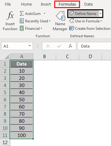
- Go to the Formula tab and click on Define Name.

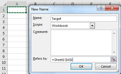
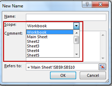
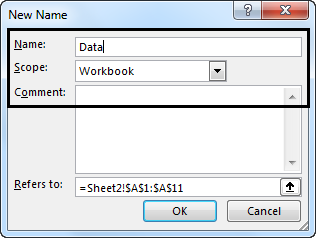
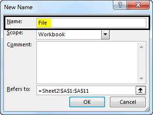
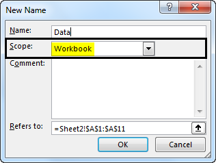
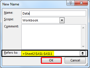
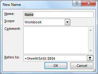
- In the New Name dialogue box type the following:
- Name: Sales
- Scope: Workbook
- Refers to: =$A$2:INDEX($A$2:$A$100,COUNTIF($A$2:$A$100,”<>”&””))

- Click OK.
- Go to the Formula tab and click on Define Name.


Done!
You now have a dynamic named range with the name ‘Sales’. This would automatically update whenever you add data to it or remove data from it.
How does Dynamic Named Ranges Work?
To explain how this work, you need to know a bit more about Excel INDEX function.
Most people use INDEX to return a value from a list based on the row and column number.
But the INDEX function also has another side to it.
It can be used to return a cell reference when it is used as a part of a cell reference.
For example, here is the formula that we have used to create a dynamic named range:
=$A$2:INDEX($A$2:$A$100,COUNTIF($A$2:$A$100,"<>"&""))
INDEX($A$2:$A$100,COUNTIF($A$2:$A$100,”<>”&””) –> This part of the formula is expected to return a value (which would be the 10th value from the list, considering there are ten items).
However, when used in front of a reference (=$A$2:INDEX($A$2:$A$100,COUNTIF($A$2:$A$100,”<>”&””))) it returns the reference to the cell instead of the value.
Hence, here it returns =$A$2:$A$11
If we add two additional values to the sales column, it would then return =$A$2:$A$13
When you add new data to the list, Excel COUNTIF function returns the number of non-blank cells in the data. This number is used by the INDEX function to fetch the cell reference of the last item in the list.
Note:
- This would only work if there are no blank cells in the data.
- In the example taken above, I have assigned a large number of cells (A2:A100) for the Named Range formula. You can adjust this based on your data set.
You can also use OFFSET function to create a Dynamic Named Ranges in Excel, however, since OFFSET function is volatile, it may lead a slow Excel workbook. INDEX, on the other hand, is semi-volatile, which makes it a better choice to create Dynamic Named Ranges in Excel.
You may also like the following Excel resources:
- Free Excel Templates.
- Free Online Excel Training (7-Part Online Video Course).
- Useful Excel Macro Code Examples.
- 10 Advanced Excel VLOOKUP Examples.
- Creating a Drop Down List in Excel.
- Creating a Named Range in Google Sheets.
- How to Reference Another Sheet or Workbook in Excel
- How to Delete Named Range in Excel?
What to Know
- Highlight the desired range of cells and type a name in the Name Box above column A in the worksheet.
- Alternatively, highlight the desired range, select the Formulas tab on the ribbon, then select Define Name.
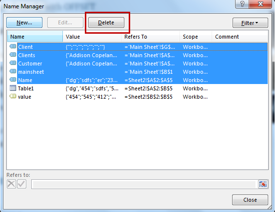
- To manage range names, go to the Formulas tab, select Name Manager, choose a name, then select Delete or Edit.
This article explains how to define and edit names for ranges in Excel for Microsoft 365, Excel 2019, 2016, 2013, and 2010.
Defining and Managing Names with the Name Box
One way, and possibly the easiest way, of defining names is using the Name Box, located above column A in the worksheet. You can use this method to create unique names that are recognized by every sheet in a workbook.
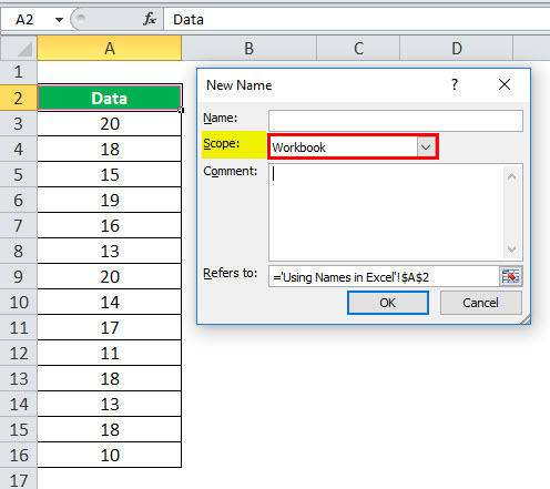
To create a name using the Name Box as shown in the image above:
-
Highlight the desired range of cells in the worksheet.
-
Type the desired name for that range in the Name Box, such as Jan_Sales.
-
Press the Enter key on the keyboard. The name is displayed in the Name Box.
The name is also displayed in the Name box whenever the same range of cells is highlighted in the worksheet. It is also displayed in the Name Manager.
Naming Rules and Restrictions
Syntax rules to remember when creating or editing names for ranges are as follows:
- A name can’t contain spaces.
- The first character of a name must be either a letter, underscore, or backslash.
- The remaining characters can only be letters, numbers, periods, or underscore characters.
- The maximum name length is 255 characters.
- Uppercase and lowercase letters are indistinguishable to Excel, so Jan_Sales and jan_sales are seen as the same name by Excel.
- Cell reference cannot be used as names such as A25 or R1C4.
What Is a Named Range?
A named range, range name, or defined name all refer to the same object in Excel; it’s a descriptive name — such as Jan_Sales or June_Precip — that is attached to a specific cell or range of cells in a worksheet or workbook. Named ranges make it easier to use and identify data when creating charts, and in formulas such as:
Additionally, since a named range does not change when a formula is copied to other cells, it provides an alternative to using absolute cell references in formulas. There are three methods for defining a name in Excel: using the name box, the new name dialog box, or the name manager.
Defining and Managing Names with the Name Manager
A second method for defining names is to use the New Name dialog box. This dialog box is opened using the Define Name option located in the middle of the Formulas tab of the ribbon. The New Name dialog box makes it easy to define names with a worksheet level scope.
To create a name using New Name dialog box:
-
Highlight the desired range of cells in the worksheet.
-
Select the Formulas tab of the ribbon.
-
Select the Define Name option to open the New Name dialog box.
-
Enter the Name, Scope, and Range in the dialog box.
-
Once completed, select OK to return to the worksheet. The name displays in the Name Box whenever the defined range is selected.
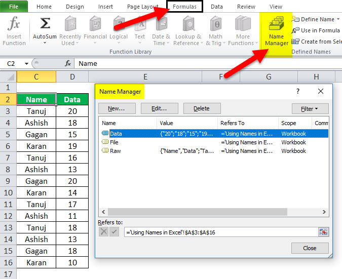
The Name Manager can be used to both define and manage existing names; it is located next to the Define Name option on the Formulas tab of the ribbon.
When defining a name in the Name Manager it opens the New Name dialog box outlined above. The complete list of steps are as follows:
-
Select the Formulas tab of the ribbon.
-
Select the Name Manager icon in the middle of the ribbon to open the Name Manager.
-
In the Name Manager, select the New button to open the New Name dialog box.
-
Enter a Name, Scope, and Range. Select OK to return to the worksheet. The name displays in the Name Box whenever the defined range is selected.
Deleting or Editing Names
With the Name Manager open:
-
In the window containing the list of names, select the name to be deleted or edited.
-
To delete the name, select the Delete button above the list window.
-
To edit the name, select the Edit button to open the Edit Name dialog box.
In the Edit Name dialog box, you can edit the chosen name, add comments about the name, or change the existing range reference.
The scope of an existing name cannot be changed using the edit options. To change the scope, delete the name and redefine it with the correct scope.
Filtering Names
The Filter button in the Name Manager makes it easy to:
- Find names with errors – such as an invalid range.
- Determine the scope of a name – whether worksheet level or workbook.
- Sort and filter listed names – defined (range) names or table names.
The filtered list is displayed in the list window in the Name Manager.
Defined Names and Scope in Excel
All names have a scope which refers to the locations where a specific name is recognized by Excel. A name’s scope can be for either individual worksheets (local scope) or for an entire workbook (global scope). A name must be unique within its scope, but the same name can be used in different scopes.
The default scope for new names is the global workbook level. Once defined, the scope of a name cannot easily be changed. To change the scope of a name, delete the name in the Name Manager and redefine it with the correct scope.
Local Worksheet Level Scope
A name with a worksheet level scope is valid only for the worksheet for which it was defined. If the name Total_Sales has a scope of sheet 1 of a workbook, Excel will not recognize the name on sheet 2, sheet 3, or any other sheet in the workbook. This makes it possible to define the same name for use on multiple worksheets – as long as the scope for each name is restricted to its particular worksheet.
Using the same name for different sheets might be done to ensure continuity between worksheets and ensure that formulas that use the name Total_Sales always refer to the same range of cells in multiple worksheets within a single workbook.
To distinguish between identical names with different scopes in formulas, precede the name with the worksheet name, such as:
Or
Names created using the Name Box always have a global workbook level scope unless both sheet name and the range name are entered into the name box when the name is defined.
Examples:
- Name: Jan_Sales, Scope — global workbook level
- Name: Sheet1!Jan_Sales, Scope — local worksheet level
Global Workbook Level Scope
A name defined with a workbook level scope is recognized for all worksheets in that workbook. A workbook level name can, therefore, only be used once within a workbook, unlike the sheet level names discussed above.
A workbook level scope name is not, however, recognized by any other workbook, so global level names can be repeated in different Excel files. For example, if the Jan_Sales name has a global scope, the same name could be used in different workbooks titled 2012_Revenue, 2013_Revenue, and 2014_Revenue.
Scope Conflicts and Scope Precedence
It is possible to use the same name at both the local sheet level and workbook level because the scope for the two would be different. Such a situation, however, would create a conflict whenever the name was used.
To resolve such conflicts, in Excel, names defined for the local worksheet level take precedence over the global workbook level. In such a situation, a sheet-level name of 2014_Revenue would be used instead of a workbook level name of 2014_Revenue.
To override the rule of precedence, use the workbook level name in conjunction with a specific sheet-level name such as:
The one exception to overriding precedence is a local worksheet level name that has a scope of sheet 1 of a workbook. Scopes linked to sheet 1 of any workbook cannot be overridden by global level names.
Thanks for letting us know!
Get the Latest Tech News Delivered Every Day
Subscribe
What is Name Range in Excel?
The name range in Excel is the range that has been given a name for future reference. To make a range as a named range, select the range of data and then insert a table. Then, we put a name to the range from the Name Box on the left-hand side of the window. After this, we can refer to the range by its name in any formula.
The name range in Excel makes it much cooler to keep track of things, especially when using formulas. You can assign a name to a range. No problem with any change in that range; you need to update the range from the Name Manager in ExcelThe name manager in Excel is used to create, edit, and delete named ranges. For example, we sometimes use names instead of giving cell references. By using the name manager, we can create a new reference, edit it, or delete it.read more. You do not need to update every formula manually. Similarly, you can create a name for a formula. Then, if you want to use that formula in another formula or another location, refer to it by name.
- The name ranges are significant because you can put any names in your formulas without considering cell references/addresses. Furthermore, you can assign the range with any name.
- Create a named range for any data or a named constant and use these names in your formulas in place of data references. In this way, you can make your formulas easier to comprehend better. A named range is just a human-understandable name for a range of cells in Excel.
- Using the name range in Excel, you can simplify and comprehend your formulas better. For example, you can assign a name for a range in an excel sheet for a function, a constant, or table data. Once you start using the names in your Excel sheet, you can easily understand these names.
Table of contents
- What is Name Range in Excel?
- Define Names For a Selected Range
- Excel names the cells based on the labels in the range you designated.
- Update named ranges in the Name Manager (Control + F3)
- How to Use Name Range in Excel?
- Example #1 Create a name by using the Define Name option
- Example #2 Make a named range by using Excel Name Manager
- Name Range using VBA.
- Things to Remember
- Recommended Articles
- Define Names For a Selected Range
Define Names For a Selected Range
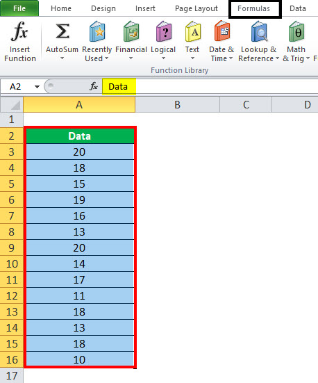
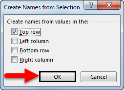
- Select the data range you want to assign a name, then select formulas and create from the selection.
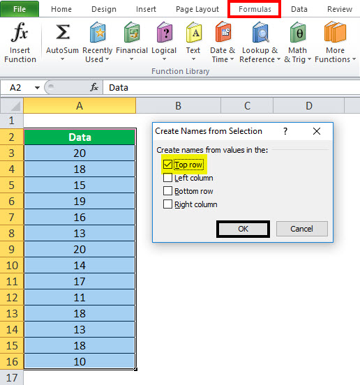
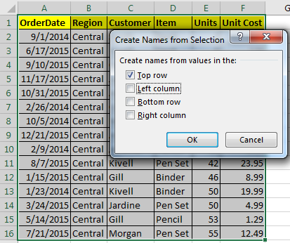
- Click on the “Create Names from Selection,” then select the “Top row,” “Left column,” “Bottom row,” or “Right column” checkbox and select “OK.”
Excel names the cells based on the labels in the range you designated.
- Use names in formulas, then select a cell and enter a formula.
- Place the cursor where you want to use the name range formula.
- Type the first letter of the name, and select the name from the list that appears.
- Or, select “Formulas,” then use in formula and select the name you want to use.
- Press the “Enter” key.
Update named ranges in the Name Manager (Control + F3)
You can update the name from the Name Manager. Press “Ctrl” and “F3” to update the name. Select the name you want to change, then change the reference range directly.
How to Use Name Range in Excel?
Let us understand the working of conditional formatting by simple Excel examples.
You can download this Using Names in Excel Template here – Using Names in Excel Template
Example #1 Create a name by using the Define Name option
Below are the steps to create a name by using the “Define Name” option:
- First, select the cell(s).

- On the “Formulas” tab, click the “Define Name” in the “Defined Names” group.

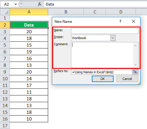
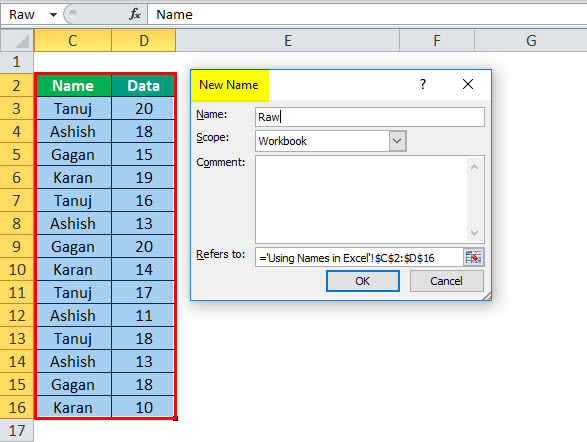
- In the “New Name” dialog box, specify three things:

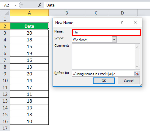
- First, in the “Name” box, type the range name.

- In the “Scope” drop-down, set the name scope (Workbook by default).

- In the “Refers to” box, check the reference and correct it if needed. Finally, click “OK” to save the changes and close the dialog box.


Example #2 Make a named range by using Excel Name Manager
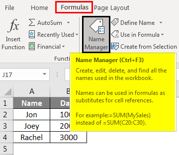
- Go to the “Formulas” tab, then the “Defined Names” group, and click the “Name Manager” or press “Ctrl + F3” (the preferred way).
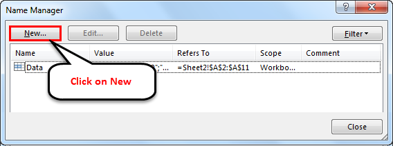
- In the top left-hand corner of the “Name Manager” dialog window, click the “New… button:”
Name Range using VBA.
We can apply the naming in VBA; here is the example as follows:
Sub sbNameRange()
‘Adding a Name
Names.Add Name:=”myData”, RefersTo:=”=Sheet1!$A$1:$A$10″
‘OR
‘You can use Name property of a Range.
Sheet1.Range(“$A$1:$A$10”).Name = “myData”
End Sub
Things to Remember
We must follow the below instruction while using the name range.
- The names can start with a letter, backslash (), or an underscore (_).
- The name should be under 255 characters long.
- The names must be continuous and cannot contain spaces and most punctuation characters.
- There must be no conflict with cell references in names using in excelCell reference in excel is referring the other cells to a cell to use its values or properties. For instance, if we have data in cell A2 and want to use that in cell A1, use =A2 in cell A1, and this will copy the A2 value in A1.read more.
- We can use single letters as names, but the letters “r” and “c” are reserved in Excel.
- The names are not case-sensitive – “Tanuj”, “TANUJ”, and “TaNuJ” are all the same in Excel.
Recommended Articles
This article is a guide to the Name Range in Excel. We discuss using names in Excel, practical examples, and downloadable Excel templates here. You also may look at these useful functions in Excel: –
- VBA RangeRange is a property in VBA that helps specify a particular cell, a range of cells, a row, a column, or a three-dimensional range. In the context of the Excel worksheet, the VBA range object includes a single cell or multiple cells spread across various rows and columns.read more
- Data Tables ExcelA data table in excel is a type of what-if analysis tool that allows you to compare variables and see how they impact the result and overall data. It can be found under the data tab in the what-if analysis section.read more
- Data Validation using ExcelThe data validation in excel helps control the kind of input entered by a user in the worksheet.read more
- Paste SpecialPaste special in Excel allows you to paste partial aspects of the data copied. There are several ways to paste special in Excel, including right-clicking on the target cell and selecting paste special, or using a shortcut such as CTRL+ALT+V or ALT+E+S.read more
While working on Excel, you must have heard about named ranges in excel. Maybe from a friend, colleague or some online tutorial. Even I have mentioned it many times in my articles. In this article, we will learn about the Named Ranges in Excel and will explore every aspect of it.
What are Named Range in Excel?
Well, named ranges are nothing but some excel ranges that a tagged with some meaningful name. For example, if you have a cell say B1, contains the everyday target, you can name that cell as specifically “Target”. Now you can use “Target” to refer at A1 instead of writing B1.
In a nutshell, Named range is just naming of ranges.
How to name a range in Excel?
Define name manually:
To define a name to a range, you can use shortcut CTRL+F3. Or you can follow these steps.
-
- Go to Formula Tab
- Locate the Defined Names section and click Define Names. It will open Name Manger.
-
- Click on New.
- Type the Name.
- Select the Scope (workbook or sheet)
- Write a comment if you want.
- In Refers to box write the reference or select a range using the mouse.
- Hit OK. It is done.
Now you can refer to it by just typing its name.
There are some rules to follow while creating names. They are
- Names should not start from digits or special characters other than underscore (_) and backslash().
- Names can’t have spaces and any special characters except _ and .
- The range should not be named as cell references. For example, A1, B1 or AZ100 etc. names are invalid.
- You can’t name a range as “r” and “c” because they are reserved for row and columns references.
- Two named ranges can’t have the same name in a workbook.
- The same range can have multiple names.
Define name Automatically
Well, most of the time you will be working with a structured data table. They will have column and rows with column headings and row headings. And most of the time these names are meaningful to the data, and you’d like to name your range as these column headings. Excel provides a tool to name ranges using titles automatically. Follow these steps.
-
- The ranges that you want to name as their headings
- Press CTRL+SHIFT+F3, or Locate Defined Names section in Formula Tab, and click Create from Selection.
-
- The below option box will appear. I selected Top Row only since I want to name these range as the heading and don’t want to name rows.
- Click OK.
Now each column is named as their heading. Whenever you typewill type a formula, these name will be listed in option to be used.
Naming Range Using Excel Tables
When we organise a data as a table in excel using CTRL + T, the column headings are automatically assigned as the name of the respective column. You should explore Excel Tables and their benefits.
How to See All Named Ranges?
Well, there will be times when you would like to see all available named ranges in the workbook. To see all name ranges Press CTRL+F3. Or you can go to Formula Tab > Name Manager. It will list all named ranges that are available on the workbook. You can Edit available named ranges, delete them, add new names.
One Range Multiple Names
Excel allows users to name the same range with different names. For example range A2:A10 can be named ‘Customers’ and ‘Clients’ both at the same time. Both names will refer to the same range A2:A10.
But you can’t have the same names for two different ranges. It eliminates the chance of ambiguity.
Get List of Named Ranges on Sheet
So if you want to have a list of named ranges and the ranges they are covering you can use this shortcut for pasting them on a place in a sheet.
-
- Select a cell where you want to get the list of named ranges.
- Press F3. This will open a Paste Name dialogue box.
- Click on paste list button.

- The list will be pasted on the selected cell and onwards.

If you double click on the named ranges name in the paste name box, they will get written as formulas in the cell. Try it.
Update Named Ranges Manually
Well, when you insert a cell inside a named range, it updates automatically and expands it. But if you add data at the end of the table, you’ll need to update the named field. To update Named Ranges, follow these steps.
- Press CTRL+F3, to open the name manager.
- Click on the named range that you want to edit. Click on Edit.
- In Refers to column type the range to which you want to expand and hit OK.
And It’s done. This is manual updating of named ranges. However, we can make it dynamic by using some formulas.
Update Named Ranges Dynamically
It is wise to make your named ranges dynamic so that you don’t have to edit them whenever your data overflows the predefined range.
I have covered it in a separate article called Dynamic Named ranges. You can learn and understand the benefits of it in detail here.
Deleting Named Ranges
When you delete some part of named range, it auto-adjusts its range. But when you delete whole name range the vanishes from the name list. Any formula, dependent on those ranges will show #REF error, or they will give incorrect output (counting functions).
For any reason, if you want to delete named ranges, follow these steps.
- Press CTRL+F3. Name manager will open.
- Select Named Ranges that you want to delete.
- Click on Delete button or hit Delete button on the keyboard.
Caution: Before you delete the named ranges, make sure that no formulas are dependent on these names. If there is any, convert them to ranges first. Otherwise you’ll see #REF error.
Deleting Names with Errors
Excel provides a tool to remove names that have errors only. You don’t need to identify each of them by yourself. To delete names with errors, follow these steps:
-
- Open Name Manager (CTRL+F3).
- Click on Filter drop-down on the right- upper corner.
- Select “Name with Errors”

- Select All and hit the delete button.
And they are gone. All the names with errors will be deleted from record immediately.
Named Ranges With Formulas
Best use of named ranges is experienced with formulas. The formulas get more flexible and readable with Named Ranges. Let’s see how.
Easy To Write Formulas
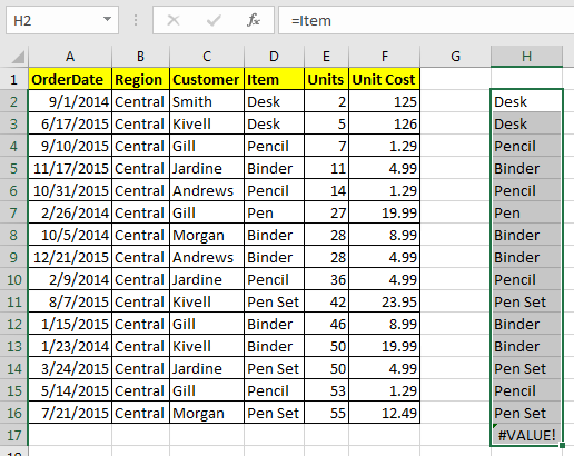
Now let’s say you have named a range as “Items”. Now the Items list you want to count “Pencils”. With name, it is easy to write this COUNTIF formula. Just write
=COUNTIF(Item, «Pencil»)
As soon as you write the opening parenthesis of formula, the list of available named ranges will appear. Without a name you would write a gi COUNTIF function of Excel with ranges, for which you may have to look at the range first then select the range or type it in the formula.
Excel Serves the Available Name Ranges.
The names of ranges are shown as suggestions when you type any letter after = sign. Same as excel shows the list of formulas. For example, if you type =u, each method and named range will be displayed starting with u, so that you can use them easily.

Make Constants using Named Ranges
So far, we learned about naming ranges, but you can actually name values too. For example, if your client name is Sunder Pichai than you can make a name “Client” and it refers to write “Sundar Pichai”. Now, whenever you write =Client in any cell, it will show Sundar Pichai.

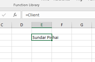
Not only text, but you can also assign a number as constant to work with. For example, you define a target. Or the value of something that will not change.
Absolute and Relative Referencing with Named Ranges
The referencing with Named ranges in is very flexible. For example, if you write the name of a named range in relative cell, it will behave like a corresponding reference. See below image.
But when you use it with formulas, it will behave as absolute. Well, most of the time you’ll be using them with formulas, so you can say that they are by default Absolute, but actually they are flexible.
But we can make them relative too.
How to make Relative Named Ranges in Excel?
Let’s say if I want to name a range “Before” which will refer to cell left to wherever it is written. How do I do that? Follow these steps:
- Press CTRL+F3
- Click on New
- Type “Befor” in ‘Name’ Section.
- In ‘Refers to:’ section write address of cell in left. For example if you are in cell B1 then write “=A2” in ‘Refers to:’ section. Make sure that it does not have $ sign.

Now wherever you will write “Befor” in formula, it will refer to cell left to it.

Here, I used before in COLUMN function. The formula returns the column number of the left cell where it is written. To my suprise, A1 shows the column number of last column. Which means the sheet is circulare. I thought it will show an #REF error.
Give Name to Often Used Formulas?
Now this one is amazing. Many times you use same formula again and again in a worksheet. For example you may want to check if a name is in your customer list or not. And this need may occur many times. For this you’ll write same complex formula every time.
=IF(COUNTIF(Customer,I3),»In List»,»Not in List»)
How about, if you just type ‘=IsInCustomer’ in a cell and it will show you if the value in left cell is in customer list or not?
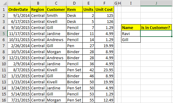
For example, I have prepared a table here. Now i just want to type “=IsInCustomer” in J5 and i would like to see if the value in I5 is in Customer list or Not. To do so follow these steps.
-
- Press CTRL+F3
- Click on New
- In Name write, ‘IsInCustomer”
- In ‘Refers To’ write your formula. =IF(COUNTIF(Customer,I5),»In List»,»Not in List»)

- Hit OK button.
Now wherever you type ‘IsInCustomer’, It will check the value in left cell in Customer list.

This stop you from repeating your self again and again.
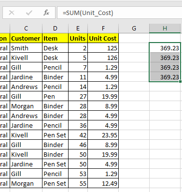
Apply Named Ranges to Formulas
So many times, we define names to our ranges after we have already written formulas based on ranges. For example I have Total Price as Cells =E2*F2. How can we change it to Units*Unit_Cost.
-
- Select the formulas.
- Go to formula tab. Click on Define Name drop down.
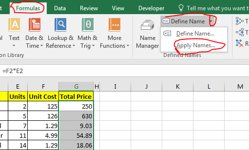
- Click on Apply Names.
- List of all named ranges will appear. Choose the right names and hit ok.
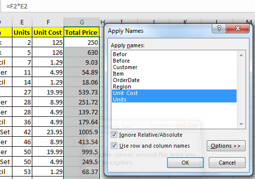
And the names are now applied. You can see it in formula bar.

Easy to Read Formulas with Named Ranges
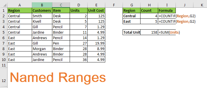
As you’ve seen that named ranges make it easy to read the formulas. If I write =COUNTIF(“A2:A100”,B2), no one will understand what I am trying to count, until they see the data or someone explains it to them.
But if I write =COUNTIF(region,’east’), most users will immediately get it that we are counting occurrence of ‘east’ in region named range.
Portable Formulas
Named ranges make it very easy to copy and paste formulas without worrying about changing references. And you can take one formula from one workbook to another and it will work fine until and unless destination workbook have same names.
Fore example if you have a Formula =COUNTIF(region,east) in Distribution Table and you have another workbook say customers that also has a named range “Region”. Now if you copy this formula directly anywhere on that workbook it will show you correct information. The structure of data will not matter. It doesn’t matter where the hell is that column in your workbook. This will work correctly.

In the above image I have used exact same formula in two different file to count number or east occuring in region list. Now they are in different columns but since both of then are named as region it will work perfectly.
Navigate Easily in Workbook
It gets easier to navigating in workbook with named ranges. You just need to type name of the named in name box. Excel will take you to the range, doesn’t matter where are you in the workbook. Given that named range is of Workbook scope.
For example, if you are on sheet10 and you want want to got customer list, and you don’t know on which sheet it is. Just go to name box and type ‘customer’. You’ll be directed to the named range in fraction of a second.
It will reduce the effort of remembering the ranges.
Navigate Using Hyperlinks with Named Range
When your sheet is large and you often go from one point to another, you like to use hyperlinks in to navigate easily. Well Named Ranges can work perfectly with Hyperlinks. To add hyperlinks using named ranges follow these steps.
-
- Choose a cell where you want hyperlink
- Press CTRL+K or go to Insert Tab> HyperLink to open Insert Hyperlink dialogue box.

-
- Click on Place in this Document.
- Scroll Down to see available Named Ranges under Defined Names

- Select the Named Range to insert a hyperlink to that range.
And its done. You have your hyperlink to your chosen named range. Using this you can create an index of named ranges that you can see and click to navigate to them directly. This will make your workbook really user friendly.
Named Range and Data Validation
Named ranges and Data Validation is kind of made for each other. Named ranges make data validation highly customisable. It gets a lot easier to add a validation from a list using named range. Let us see how..
-
- Go to Data tab
- Click on Data Validation
- Select List in ‘Allow:’ section
- In ‘Source:’ section, type “=Customer” (write whichever named range you have)

- Hit OK
Now this cell will have names of customers who are part of Customer named range. Easy, isn’t it.
Dependent or Cascading Data Validation with Named Ranges
Now what if you want a cascading or dependent data validation. For example, if you you want a drop down list that has categories, Fruits and Vegetables. Now if you choose fruits than another drop down should show only fruits option and if you choose Vegetable then only vegetables.
This can be easily achieved by using Named ranges. Learn how.
- Dependent Drop down using Named Range
- Other Ways for Cascading Data Validation
No Data Validation With Names of Tabled Data
Although Excel Tables provide structured names but they can not be used with data validation and Conditional Formatting. I don’t know why excel doesn’t allow it.
But it doesn’t mean that it can’t be done. You can name ranges within a table and then use them for validation. Excel does not have any problem with it.
Scope of Named Ranges
So far we talked about named ranges that had Workbook scope. What? We we didn’t discussed it? Ok, so lets quickly understand what Scope of named ranges are.
What is Scope of a Name Range?
Well scope defines where a name range can be recognised. Any name can not be recognised out its scope. For example a name in workbook1 can not be recognised in different workbook. Excel provides two options for scope of named ranges Worksheet and Workbook.
How to define a Scope of Named Range?
When you create a new name range, you can see a ‘Scope:’ section. Click on the drop down and choose the scope for your name range. You can’t change scope once you have created a named range. So better do it before. By default, it is workbook.
Workbook Scope
This is the default scope for a named range. A name defined with scope of workbook can be used in whole workbook in which it is defined (not other workbooks).
All above examples had workbook scope.
Worksheet Scope
A name that is define with a worksheet scope can only be used on define worksheet. For example if I define ‘Total’ for a total cell with scope of sheet1. Then total will be recognised on sheet1 only. Other sheets will not recognise.
I Want a Excel Scope
Excel does not have Global or say Excel Scope. Actually, I would like to define some names that can be recognised in all workbooks on my system. If anyone knows how can we do this, let me know.
Editing Scope After Creating Names
You can’t. Excel does not allow you to edit scope of a named range once you have create. Since all named ranges on a sheet are by default Workbook Scoped, and you may want to change their scope to a sheet.
To do so, just make a copy of that sheet and excel will make each name on that sheet local to avoid ambiguity. You can now delete the original sheet if you like.
Cut Paste Name Range
When you cut and paste a named range from one destination to another, the reference changes to new location. For example if you have a named range “Customer” in A2:A10 and cut and paste it to B2:B10, then customer name will refer to new location B2:B10.
Related Article:
Dynamic Named Ranges in Excel
17 Amazing Features of Excel Tables
Popular Articles:
50 Excel Shortcuts to Increase Your Productivity
How to use the VLOOKUP Function in Excel
How to use the COUNTIF function in Excel
How to use the SUMIF Function in Excel
Names are one convenient identity. Imagine how we’d be addressed if we didn’t have names? Excel tries to make our lives easier by providing us with a similar convenience.
Excel’s Names feature can be surprisingly powerful for organizing data in Excel. Named Ranges let you name a group of cells and then refer to them as a unit as if they were a single cell.
Using named ranges can make formulas easier to read and understand and provides simple navigation via the Name Box. Named ranges are easy to create and can be used for a variety of purposes.
This tutorial will teach you how to use Names feature in Excel.

What are Named Ranges
In Excel, a cell or a range of cells can be named to make their usage easier. It would be simpler to use a named range directly in a formula or select said range.
You can name:
- a Range of cells,
- a Formula,
- a Constant or
- a Table
Benefits of Creating Named Ranges in Excel
- The prime advantage of named ranges is the ease they provide. You don’t have to keep glancing at certain cells or tables to pick up values or cell references and can use a named range instead.
- Using a named range will save typos that may otherwise occur while typing values or formulas since entering named ranges is a clickable option.
- They are of great help to use in formulas as the named range appears upon typing the first letter of the name.
- Named ranges make formulas movable and they can be used from sheet to sheet and workbook to workbook.
- A dynamic named range can automatically account for expanding and contracting data (when values are added or deleted from a dataset) without having to change the formula or recalculate.
- A named range can be used for data validation (creating drop-down menus) without much hassle.
- Hyperlinks can quickly be created from existing named ranges.
- Named ranges make navigation and directing very easy. You can click on a named range in the Name Box and arrive at the named range.
- For all the above benefits that named ranges deliver, they are very simple and quick to create.
Rules for naming Named Ranges
There are several pointers not to trespass while creating named ranges:
- A name should have less than 255 characters.
- A name should not have space and punctuation characters (exceptions mentioned as follows).
- A name’s first character has to be a letter, an underscore ( _ ), or a backslash ( ).
- A name may contain a question mark but never as a first character.
- A name is not case-sensitive. (sale, Sale, and SALE are treated as one name).
- A name must not resemble a cell reference (e.g., A1, A$1).
- A name may be a single letter name but must not be r, R, c, or C as «R» and «C» signify row and column selection shortcuts.
How to Create Named Ranges in Excel
There are two methods to create named ranges in excel. We will see both these methods in this section.
Let’s say we have the data as shown below and we want to create two named ranges – one for the History marks and the second one for the Geography marks.

We will create these two named ranges using two different methods to help you get a hang of both methods.
Method 1 – Creating Named Ranges from the Name Box
The how-to here is pretty simple. Select the range, enter the desired name in the «name box» and press Enter. Done! Really! We can show you how easy this is with a visual.
Here’s how it’s done:
- For naming the History marks range, we will select the History marks i.e., range C3:C7.

- Click on the name box.
- Enter the desired name («History» in this case).

- Press the Enter key.
Method 2 – Creating Named Ranges from the ‘Define Name’ Option
Names can also be created from the «Define Name» button, in the formulas tab. To use this method follow the below steps:
- Select the range which you want to name, in our case it will be D3:D7.
- Navigate to the «Formulas Tab» and click the «Define Name» button.

- Now, in the «New Name» window enter the desired name for the named range.

- After entering the desired name click the «OK» button and it is done.
How to Edit Named Ranges in Excel
Suppose you accidentally missed a cell in the range or want to change the name of your named range. This means the named range needs to be edited.
Named ranges can be managed through the «Name Manager» which can be found under the «Formulas» tab > Name Manager or can be accessed through the keyboard shortcut Ctrl + F3.

This is what you will see when you open the Name Manager:

Here, you can see the named ranges in your sheet and their details. Double click the named range you wish to edit or select the named range and click the «Edit…» button.

Clicking on the «Edit…» button will open the «Edit Name» window where you can edit the name or the cell range of the named range. When done, click «OK» and then click the «Close» button on the Name Manager.
How to Delete Named Ranges
The Name Manager can also be used to delete named ranges. Click the named range you wish to remove, press the «Delete» button.

You will get a pop-up confirmation asking whether you want to delete the named range or not. Press «OK» and that will delete your chosen named range.

Note that the Name Manager also has a «Filter» button that can be used for filtering the names and only viewing the relevant names at a given time. It can be quite handy when you have a lot of names to deal with.
Recommended Reading: How to Lock and Protect Cells in Excel
How to Create Names from Cell Text
For batch information where the data is in the columnar or row format (i.e., in either columnar form with headings at the top and its relevant data below. Or in rows with headings on the left and its data on the right) there is a quicker way of naming ranges. We can use the «Create from Selection» feature in Excel to give the heading’s name to the range. Here is how:
So, we have the dataset containing marks scored by students in various subjects. The layout is in columnar form. We can use the «Create from Selection» feature in this case as –

- Select the range and the heading. We will select columns C, D, E, and F to name each range according to its heading.

- In the «Formulas» tab, click «Create from Selection» or use the keyboard shortcut Ctrl + Shift + F3. This is what you should see:

- According to the layout of your dataset, select the row or column where the headings need to be picked from. For our case, we will select the «Top row» option as headings. «Marks in History», «Marks in Geography», «Marks in Science», and «Marks in Math» are in the top row.
- After selecting the appropriate options click «OK».
Doing this has created multiple named ranges for our data. You can see from the drop-down in the Name Box that we have 4 named ranges created according to the headings of each column.

Note that the spaces in headings are replaced with underscores while creating the names.
Named Ranges with Hyperlinks
If you thought named ranges made you bounce around with ease through worksheets, wait for their synergy with hyperlinks. Named ranges make hyperlinking a smoother process as data required for hyperlinking would already be grouped and named. Let’s show you how this will work.
For the sake of this example let’s assume that we have another named range «Student» in Sheet2 as shown.

We will hyperlink the Student column from Sheet1 to direct us to the student range in Sheet2.
- Select the Student range in Sheet2 (i.e., B3:B7).

- Right-click the selected area and click on «Link». The «Insert Hyperlink» window is what you should see.

- We will select «Student» from «Defined Names» which we have already defined in Sheet2.
- Click «OK».

We have hyperlinked the Student Names to Sheet2 using the «Student» named range. Clicking on any of the marks should take us to the «Student» range on Sheet2. Let’s check.

Affirmative!
How to Create an Excel Name for a Constant
The Name Manager can also be used to create a name for a constant value. This constant value will not be a cell reference on the sheet but it can be used by its name in formulas.
For our example, we will use a named constant to calculate the percentage of the overall marks of each of 5 students. We start by accessing the Name Manager and applying for a new name.

The percentage will be calculated by dividing the sum of the attained marks by the total (each subject is marked out of 50. Which makes 50 x 4 = 200). We will set «200» as our named constant and give it the name «total».
Using «total», we can calculate the percentages without having to refer to «200».

Here, we have substituted «200» for «total» and calculated each student’s overall percentage.
How to Make a Named Formula
Taking the above example, what if we named the whole formula and get the same results? Sounds like a good bargain for smart input. Let’s see how to do that.
We first head to good old Name Manager and «New Name» again. We will name our formula «Percentage». The reference of this name is shown as
=SUM(Sheet2!$C3:$F3)/total

The range of the SUM in the formula is «C3:F3». The columns have been locked into absolute references by the $ sign. Notice that the rows have not been locked as absolute references so that the formula can be dragged to apply to all the rows.

Now just by using «Percentage», we can use the named formula to calculate the students’ percentages.
Named Ranges for Data Validation
Named ranges make the «Data Validation» feature in Excel a breeze. You can create a drop-down menu with values from a named range.
This comes with some advantages. You can simply refer to the named range in the Data Validation window instead of having to directly enter the cell ranges. It also gives a point of relevance to see the named range in sight. Let’s see how it’s done.
Let’s assume – we have a list of products and their prices and discounts. Our objective here is to calculate the discounted price for each product after entering its relevant discount. Instead of copy-pasting each discount, we want the option to select the discount from a drop-down menu for each cell in column D.

We will create a drop-down menu with the «Discount» named range (G3:G6).
- Select the cells for which you want to create the drop-downs (D3:D9 for our case).

- Under the «Data» tab, in the «Data Tools» section, select «Data Validation» dropdown and click the next «Data Validation» option.
- Inside the «Data Validation» window, under «Allow», choose «List» and enter the required named range under «Source». We will enter the reference of our «Discount» range here.

- Click «OK». This has very conveniently created drop-down menus for all cells D3:D9, taking values from the «Discount» named range.

- Now we can select the respective discounts and arrive at our «Price after discount».
See all Names Directly on the Worksheet
There is a small hack that allows you to see all the names directly on the worksheet. You can view all your named ranges (marked with the names) on the sheet if you zoom out to anything less than 40%. We’ll follow that religiously and zoom out at 39%.

The only thing amiss about this is that the named range text is like a watermark; it’s not opaque and will not work so well for small and narrow columns. This hack is suitable for data with a wide-set column or several more rows so the name of the range can be seen. Otherwise, it would be on the brink of being unnoticeable.
Scope of a Name
If you open the Name Manager and have a look at the named ranges, you will find that each named range has a scope (e.g., Sheet1, Sheet2, Workbook, etc.) against it.

Scope refers to the location, or level, within which the name is recognized. For instance, in the above image «range4» can only be used within Sheet1 whereas all the other names can be used across the entire workbook.
Based on this there can be 2 levels of scopes:
- Local worksheet scope
- Global workbook scope
Local Worksheet Scope
Locally scoped names can only be recognized and used on the sheet it is created upon. This implies that inside a single workbook we can have the same locally scoped names (each within a separate worksheet). For instance – you can have a yearly expense workbook with a worksheet for each month and then we can have a single locally scoped name within each worksheet.
Pro Tip: Named ranges made using the Name Box have global scope by default. However, you can tie the named range down to a sheet (in other words, make it locally scoped) simply by using the sheet’s name before the range’s name (with an exclamation mark).
Sheet1!Expenses
Global Workbook scope
Globally scoped names can be recognized and used across the whole workbook. Global names must always be unique within the workbook. For instance – we can create a global name to define the value of a constant like pi (as 3.14) and use it across the whole workbook.
Creating Dynamic Named Ranges in Excel
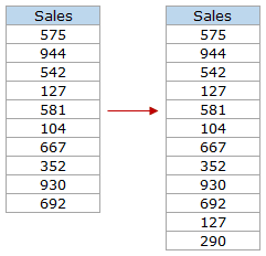
Up until now with all the examples above, we can say that if we were to expand on the data by adding more values, the formulas already applied wouldn’t account for the new values. This means that whenever values will be added to the dataset of the named range (e.g., B2:B15) which expands the dataset to B2:B20, the named range will still not account for the additional 5 values and remain a named range for B2:B15. This means the named range is static as opposed to a dynamic named range. The additional step that would need to be taken to fix this is to edit the named range and modify the range mentioned.
A dynamic named range on the contrary will itself adjust for changes in the range. To make our named range dynamic, we will add a function to the reference of the named range. If this sounds too complicated, let us show you how it’s done.
There are a couple of ways of creating a dynamic named range. One of them is using the OFFSET function. The drawback is however that OFFSET is a volatile function; with each and every change in a worksheet, OFFSET recalculates. This is not an issue for an uncomplicated worksheet with small datasets. But with complex and large worksheets, you will find that OFFSET slows things down. In such a case, the other way to create a dynamic named range is using the INDEX function.
So if you can use OFFSET for small datasets and INDEX for large ones, why not just master the INDEX function and use that? So this use of the INDEX function for dynamic named ranges is what we’ll be tapping into right now. Let’s see an example:

Taking simple sales data, we will add a dynamic named range that we will later use to calculate the total sales:
- Open the «Name Manager» > click the «New Name» option.
- Set the desired name (we are naming our named range «Sales»).

- In «Refers to», feed the following formula, and click «OK».
=$C$3:INDEX($C$3:$C$1048576,COUNTIF($C$3:$C$1048576,"<>"&" "))

We have used the SUM function to total the named range «Sales». It has given us a total of «3186» which is also confirmed from selecting the cells with the results displayed in the status bar below.
Now let’s add some values to this dataset to see if the formula applied complies with changes in the data.

We have added new sales data and the named range has updated itself because of the formula we have put in to build the range. So how does this formula work?
Let’s see the formula again:
=$C$3:INDEX($C$3:$C$1048576,COUNTIF($C$3:$C$1048576,"<>"&" "))
Since we’re using the INDEX function in the formula, let’s get familiar with it. The INDEX function returns a value or cell reference of a particular cell in a given range. The part we need to work with right now is the return of a cell reference.
The COUNTIF function counts the number of cells within a range that meets the given condition. The range given to COUNTIF is C3:C1048576. COUNTIF needs to look through the entire C column ahead of C3 (if you press Ctrl + down key, you will find the last row given in Excel which is row number 1048576. That is why we have used C1048576 in our formula. According to how big or small your data is, you can refer to any row ahead of your last value, suppose 100 rows ahead of your last value. In this way the formula will account for all changes made up to the last-mentioned row).
The condition given to COUNTIF is counting the number of cells from C3 to C1048576 that should not be equal to (defined by «<>») blank cells (defined by » «). Take note that this will work only if the data does not consist of blank cells as the blank cells are the ones to be ignored by the function.
According to this condition, the non-blank cells that COUNTIF was able to find from the given range were C3:C9. Passing this result to the INDEX function, INDEX then returns the value of the last item of the list (which would be C9’s value i.e., 404). The formula starts with the first cell that we need to include in our named range (i.e. C3, fed as an absolute reference by «$» signs). Using this reference before the INDEX function makes INDEX return the cell reference instead of the value which will then be C9.
The result of the whole formula has worked like this:

Note: Dynamic named ranges aren’t shown in the Name Box. Use the Name Manager to see all named ranges (static and dynamic).
Named Range Shortcuts
The more matters are sitting on your fingertips, the better. To wrap things up, here are some useful keyboard shortcuts with named ranges that should move you around the sheet even faster.
- F3 – Pops up a «Paste Name» dialogue box for pasting a named range from the full list of named ranges.
- Ctrl + F3 – Opens «Name Manager»
- Ctrl + alt + F3 – Pops up «New Name» dialog box for creating a new named range.
- Ctrl + shift + F3 – Pops up «Create Names from Selection» dialog box for creating named ranges from headings/titles.
- F5 – Pops up the «Go To» dialog box for navigating to the chosen named range from the full list of named ranges.
With that, we’ve discussed the ins and outs of the Named Ranges in Excel. They are simple, but extremely useful while working with larger datasets and multiple ranges. While you solidify your expertise with some practice, we’ll have another awesome tutorial ready for you ready!
Excel Named Range (Table of Contents)
- Named Range in Excel
- Define Names from a Selected Range
- How to Create a Named Range in Excel?
Introduction to Named Range in Excel
Named Range just makes the process of working with formulas exciting, especially to keep track of things. It is just very convenient to assign a name to a range. If there is any change in that range, it becomes infinitely easier to update the range through the Name Manager. It totally allows us to bypass the process of manually updating every formula. Also, in cases of nested formulas, where one formula has to be used in another formula or maybe just used in a different location, all that needs to be done is to refer to the formula by its name.
The importance of named ranges is that one can use any names in the formula without worrying about the cell addresses/references. Any name can be assigned to a range. Any named constant or any data can be given a named range, and these names can be used instead of the actual formula. In this way, it becomes easier to understand the formulas. So, what this does is that it gives a range of cells in Excel a human-understandable name. By making use of named ranges, one can make the usage of formulas straightforward in Excel. One can give a name to a range in a formula or function, a constant, or a table. After starting to use names in a sheet, one can easily comprehend these names.
Define Names from a Selected Range
Firstly, one has to select the range that you want to give a name. Thereafter navigate to Formulas and then select Create from Selection.
From the “Create Names from Selection” box, select either Bottom Row, Top Row, Left Column, or Right Column, and then click on OK.
The cells are named based on labels in the designated range:
- First, use names in formulas and then focus on a cell and then enter a formula.
- The cursor has to be placed at the location where we want to use the named range in a formula.
- The name can be selected from the list that opens up after typing the name’s first letter.
- Alternatively, navigate to Formulas and then Use in Formula, followed by selecting the name that you intend to use.
- Press Enter.
It is also possible to update the named ranges from the Name Manager. The shortcut to update the named ranges from the Name Manager is Ctrl+F3. We just need to select the name that we wish to change and then proceed to change the reference directly.
How to Create Named Ranges in Excel?
Let us understand the concept of the Named Range through some examples.
You can download this Named Range Excel Template here – Named Range Excel Template
Example #1
Create a Named Range by using the Define Name option
- First, focus on the cells by selecting the range of cells.
- Now, navigate to the Formulas tab. Next, go to the Defined Name group. Click to select Define Name.
- Now once the New Name dialog box opens, mention three things -Name, Scope, Comment.
- Now in the “Name:” category, provide a name for the range.
- Now in the “Scope:” category, from the dropdown, the name scope has to be set (by default, it is Workbook)
- Now move on to the ‘Refers to:’ section, verify the available reference, and modify it if required. After that, click on OK to save the changes you have made and close the dialog box.
Example #2
Create a Named Range by utilizing the Name Manager
- Navigate to the Formulas tab and then proceed towards Define Name Group and then click on Name Manager.
- Alternatively, you can also press Ctrl+F3, which is the shortcut for the same.

- Now, on the top, towards the Name Manager’s left corner, we have the ‘New’ button. Click on it.
Then the New Name dialog box will open.
Example #3
Create a Named Range using VBA
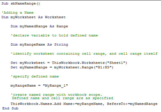
We can also create a Named Range in VBA.
So, this is what we did in the code snippet above:
- We created three variables – myWorksheet of Worksheet datatype, which will store the name of the Excel Worksheet, myNamedRange of Range datatype, which will hold the name of the range of cells that we wish to name, and myRangeName, of String datatype, which will hold the name of the Named Range.
- We defined our Worksheet (in the variable myWorksheet).
- We then went on to define the range of cells that we wanted to name (in the variable myNamedRange).
- After that, we defined the name of our Named Range in the variable myRangeName.
- After that, we proceed to create the Named Range and provide the reference to which it will point to.
This concludes the Named Range creation process through VBA.
Things to Remember
The following things must always be kept in mind while creating or dealing with Named Ranges in Excel.
- Named Ranges can have names that start with either a backslash (), letter, or underscore (_). Numbers or other special symbols are invalid as the starting character. If any other character other than letters, backslash or an underscore is given as the starting character, then Excel will throw an error.
- There is also a limitation on how long the name of a Named Range can be. The maximum length of a name can be 255 characters. Anything above 255 characters will cause Excel to throw an error.
- Every name has to be a continuous sequence of characters. There is no scope to have spaces, tabs, or any punctuation marks in the name. This is done so as to maintain uniformity and make the names easier.
- Another important instruction while working with Named Ranges is that a Named Range’s name must not have any conflict with cell references.
- As we saw, there is a limit on the maximum length for a name. Conversely, a name must also be of at least one character length at a minimum. Names are allowed to be of a single character length; however, there are few characters such as ‘r’ and ‘c’, which are reserved by Excel and can not be used as Names.
- As a bonus, Names aren’t case sensitive, which means that names such as “Jon”, “JON”, “jon” are all the same to Excel.
Recommended Articles
This has been a guide to Named Range in Excel. Here we discussed how to create a named range in excel along with practical examples and a downloadable excel template. You can also go through our other suggested articles to learn more –
- Excel Function for Range
- Range in Excel
- VBA Named Range
- VBA Range
We can use the name for the cell Ranges instead of the cell reference (such as A1 or A1:A10). We can create a named range for a range of cells and use then use that name directly in the Excel formulas. When we have huge data sets, Excel-named ranges make it easy to refer (by directly using a name to that data set).
Creating an Excel Named Range :
There can be 3 ways to create named ranges in Excel :
Method 1: Using Define Name
Use the following steps to create named range using Define Name :
- Select the range B1:B5.
- Click on the Formulas tab.
- Then click on Define Name.
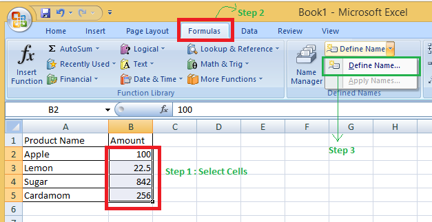
- Give a new Name(PriceTotal in our example) & click Ok. (You can see the range in the bottom refers to section, here absolute referencing is used, $ before the row number/ column letter locks the row/column).

- Now, the next thing is to see that how to use this named range in any of the Excel formulas. For example, if you want to get the sum of all numbers in the above name range then, can say simply write: =SUM(PriceTotal).

Here, B7 =SUM(PriceTotal) = 100 + 22.5 + 843 + 256 (all the numbers in the named range)= 1220.5
Note: The named Range created by this method is restricted to a worksheet.
Method 2: Use the Name Box
Use the following steps to create a named range using the name box :
- Choose the range for which you’d want to give it a name (not the headers).
- Type the name of the range with which you wish to construct the Named Range in the Name Box on the left of the Formula bar.

Note: The Name created this way is available in the entire excel current Workbook.
Method 3: From Selection Option
When you have tabular data and wish to construct named ranges for each column/row, this is the preferred method.
Example: We have 3 columns having headers: Product Name, Amount & Tax Percent.
Use the following steps to create a named range from the selection option :
- Select the complete data set (the 3 columns with the headers).
- Click on the Formulas tab.
- Click Create from Selection (or press Control + Shift + F3).

- After the click, Create Names from Selection’ dialogue box will be opened.

- Check the settings where you have the headers in the Create Names from Selection dialogue box. Because the heading is in the top row, we only select the top row. You can choose both if you have headers in the top row and left column. We only need to check the Left Column option, if the data is organized with the headers only in the left column.
Here we select only Top row because we have headers in the top row.
Result: The data set you selected in column A will be having a named Range: Product_Name (Spaces not allowed, so underscore automatically replaces space)
The data set you selected in column B will be having a named Range: Amount
The data set you selected in column C will be having a named Range: TAX_Percent (Spaces not allowed, so underscore automatically replaces space)
Benefits of Creating Named Ranges in Excel:
The following are benefits of creating & use Named Ranges in Excel :
Instead of using cell references every time, we can directly use Named Reference
Example 1: In the above example, to calculate the sum, we used B7 =SUM(PriceTotal) instead of B7 = SUM(B2:B5) for the above data range.
Example 2: If for the same-named Range, if we write, B9 = SUMIF(PriceTotal,”>50″), then the sum will be equal to the sum of all numbers > 50 in the named range.
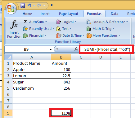
Here, sum is done for all the numbers > 50 in the named range “PriceTotal” = 100+842+256 = 1198.
- To Select Cells, you do not need to return to the data set to choose the cells. You can directly use the Named range, by typing the first few characters of the named range, excel shows a list of named ranges that matches the typed characters.
Example :

As you can see that after just typing Pr, a drop-down list for the available options(formula & named Range) is pooped up.
- The formulas become dynamic using named Ranges:
- Excel formulas become dynamic if we use Named Ranges. In the above example, if we add another cell of Tax Percent (2.5%)& you name it as “TAX” . Now to calculate Final Price (including tax), we can use the Named Range instead of using the value 2.5.
- Now, if later tax is increased to 3%, you just have to update the Named Range, and all the calculations would be done automatically & we will get the Final Price according to the latest tax percent.
- Finding a named cell is less time-consuming.
Using Create From Selection Option :
When generating Named Ranges in Excel, you should be aware of the following naming conventions:
- A letter and underscore character(_), or a backslash, shall be the initial character in a Named Range (). It will display an error if it is anything else is used. Letters, numbers, special characters, a period, or an underscore can make up the remaining characters.
- When establishing named ranges, you can’t use spaces. Tax Percent, for example, cannot be a named range. We can use an underscore, a period, or capital characters if we wish to make a Named Range out of two words, You may, for example, Tax_Percent, TaxPercent, etc.
- In Excel, you can’t use names that are also cell references. You can’t use C1 because it’s also a cell reference.
- You can only have a maximum of 255 characters in a named range.
- For Excel, uppercase and lowercase letters are the same when generating named ranges. For example, if you create a named range called ‘TAX’, you cannot create another named range called ‘Tax’ or ‘tax’.
Name Rows and Columns in Excel:
You may find yourself producing a lot of Named Ranges in Excel when working with large data sets and complex models. It is possible that you can’t recall the name of the Named Range you made. What to do then?
Solutions:
1. Getting the Names of All the Named Ranges
- Click on the formula tab.
- Choose – Use in Formula(In the Defined Named group).

- Choose Paste names & you will get a list of all the Named Ranges in the workbook.

2. Displaying the Matching Named Ranges
As discussed earlier, type a few initial characters, if you have some glimpse about the Name, and a drop-down list of matching ones will be shown.
Editing the Named Range in Excel :
To change/ edit the already created named range, follow these steps :
- Click the Formulas tab.
- Click the name manager(or Ctrl + F3).

- All of the Named Ranges in that workbook will be listed in the Name Manager dialogue box. Double-click the Named Range you’d like to change.

- Edit Name dialog box will pop up, make the modifications.
Example:
Here when we double-click Amount, the edit window for the same get open & we rename that named range from Amount to any other name.

- Click OK and close the name manager window.
Useful Named Range Shortcuts:
When dealing with Named Ranges in Excel, the following keyboard shortcuts can come in use frequently :
- F3: Will give a list of all the Named Ranges and pasting it in any Formula.
- Ctrl + + Shift + F3 : To pop up create Named Ranges from Selection window.
- Ctrl + F3 : To pop up the name manager window directly.
- F1: For Excel Help.