
Use LOOKUP, one of the lookup and reference functions, when you need to look in a single row or column and find a value from the same position in a second row or column.
For example, let’s say you know the part number for an auto part, but you don’t know the price. You can use the LOOKUP function to return the price in cell H2 when you enter the auto part number in cell H1.
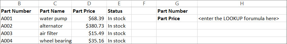
Use the LOOKUP function to search one row or one column. In the above example, we’re searching prices in column D.
Tips: Consider one of the newer lookup functions, depending on which version you are using.
-
Use VLOOKUP to search one row or column, or to search multiple rows and columns (like a table). It’s a much improved version of LOOKUP. Watch this video about how to use VLOOKUP.
-
If you are using Microsoft 365, use XLOOKUP — it’s not only faster, it also lets you search in any direction (up, down, left, right).
There are two ways to use LOOKUP: Vector form and Array form
-
Vector form: Use this form of LOOKUP to search one row or one column for a value. Use the vector form when you want to specify the range that contains the values that you want to match. For example, if you want to search for a value in column A, down to row 6.

-
Array form: We strongly recommend using VLOOKUP or HLOOKUP instead of the array form. Watch this video about using VLOOKUP. The array form is provided for compatibility with other spreadsheet programs, but it’s functionality is limited.
An array is a collection of values in rows and columns (like a table) that you want to search. For example, if you want to search columns A and B, down to row 6. LOOKUP will return the nearest match. To use the array form, your data must be sorted.
Vector form
The vector form of LOOKUP looks in a one-row or one-column range (known as a vector) for a value and returns a value from the same position in a second one-row or one-column range.
Syntax
LOOKUP(lookup_value, lookup_vector, [result_vector])
The LOOKUP function vector form syntax has the following arguments:
-
lookup_value Required. A value that LOOKUP searches for in the first vector. Lookup_value can be a number, text, a logical value, or a name or reference that refers to a value.
-
lookup_vector Required. A range that contains only one row or one column. The values in lookup_vector can be text, numbers, or logical values.
Important: The values in lookup_vector must be placed in ascending order: …, -2, -1, 0, 1, 2, …, A-Z, FALSE, TRUE; otherwise, LOOKUP might not return the correct value. Uppercase and lowercase text are equivalent.
-
result_vector Optional. A range that contains only one row or column. The result_vector argument must be the same size as lookup_vector. It has to be the same size.
Remarks
-
If the LOOKUP function can’t find the lookup_value, the function matches the largest value in lookup_vector that is less than or equal to lookup_value.
-
If lookup_value is smaller than the smallest value in lookup_vector, LOOKUP returns the #N/A error value.
Vector examples
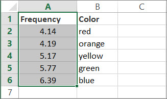
You can try out these examples in your own Excel worksheet to learn how the LOOKUP function works. In the first example, you’re going to end up with a spreadsheet that looks similar to this one:
-
Copy the data in following table, and paste it into a new Excel worksheet.
Copy this data into column A
Copy this data into column B
Frequency
4.14
Color
red
4.19
orange
5.17
yellow
5.77
green
6.39
blue
-
Next, copy the LOOKUP formulas from the following table into column D of your worksheet.
Copy this formula into the D column
Here’s what this formula does
Here’s the result you’ll see
Formula
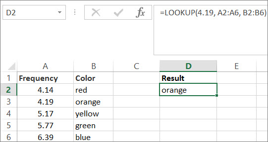
=LOOKUP(4.19, A2:A6, B2:B6)
Looks up 4.19 in column A, and returns the value from column B that is in the same row.
orange
=LOOKUP(5.75, A2:A6, B2:B6)
Looks up 5.75 in column A, matches the nearest smaller value (5.17), and returns the value from column B that is in the same row.
yellow
=LOOKUP(7.66, A2:A6, B2:B6)
Looks up 7.66 in column A, matches the nearest smaller value (6.39), and returns the value from column B that is in the same row.
blue
=LOOKUP(0, A2:A6, B2:B6)
Looks up 0 in column A, and returns an error because 0 is less than the smallest value (4.14) in column A.
#N/A
-
For these formulas to show results, you may need to select them in your Excel worksheet, press F2, and then press Enter. If you need to, adjust the column widths to see all the data.
Array form
The array form of LOOKUP looks in the first row or column of an array for the specified value and returns a value from the same position in the last row or column of the array. Use this form of LOOKUP when the values that you want to match are in the first row or column of the array.
Syntax
LOOKUP(lookup_value, array)
The LOOKUP function array form syntax has these arguments:
-
lookup_value Required. A value that LOOKUP searches for in an array. The lookup_value argument can be a number, text, a logical value, or a name or reference that refers to a value.
-
If LOOKUP can’t find the value of lookup_value, it uses the largest value in the array that is less than or equal to lookup_value.
-
If the value of lookup_value is smaller than the smallest value in the first row or column (depending on the array dimensions), LOOKUP returns the #N/A error value.
-
-
array Required. A range of cells that contains text, numbers, or logical values that you want to compare with lookup_value.
The array form of LOOKUP is very similar to the HLOOKUP and VLOOKUP functions. The difference is that HLOOKUP searches for the value of lookup_value in the first row, VLOOKUP searches in the first column, and LOOKUP searches according to the dimensions of array.
-
If array covers an area that is wider than it is tall (more columns than rows), LOOKUP searches for the value of lookup_value in the first row.
-
If an array is square or is taller than it is wide (more rows than columns), LOOKUP searches in the first column.
-
With the HLOOKUP and VLOOKUP functions, you can index down or across, but LOOKUP always selects the last value in the row or column.
Important: The values in array must be placed in ascending order: …, -2, -1, 0, 1, 2, …, A-Z, FALSE, TRUE; otherwise, LOOKUP might not return the correct value. Uppercase and lowercase text are equivalent.
-
This Excel tutorial explains how to use the Excel LOOKUP function with syntax and examples.
Description
The Microsoft Excel LOOKUP function returns a value from a range (one row or one column) or from an array.
The LOOKUP function is a built-in function in Excel that is categorized as a Lookup/Reference Function. It can be used as a worksheet function (WS) in Excel. As a worksheet function, the LOOKUP function can be entered as part of a formula in a cell of a worksheet.
There are 2 different syntaxes for the LOOKUP function:
LOOKUP Function (Syntax #1)
In Syntax #1, the LOOKUP function searches for value in the lookup_range and returns the value in the result_range that is in the same position.
The syntax for the LOOKUP function in Microsoft Excel is:
LOOKUP( value, lookup_range, [result_range] )
Parameters or Arguments
- value
- The value to search for in the lookup_range.
- lookup_range
- A single row or single column of data that is sorted in ascending order. The LOOKUP function searches for value in this range.
- result_range
- Optional. It is a single row or single column of data that is the same size as the lookup_range. The LOOKUP function searches for the value in the lookup_range and returns the value from the same position in the result_range. If this parameter is omitted, it will return the first column of data.
Returns
The LOOKUP function returns any datatype such as a string, numeric, date, etc.
If the LOOKUP function can not find an exact match, it chooses the largest value in the lookup_range that is less than or equal to the value.
If the value is smaller than all of the values in the lookup_range, then the LOOKUP function will return #N/A.
If the values in the LOOKUP_range are not sorted in ascending order, the LOOKUP function will return the incorrect value.
Example (as Worksheet Function)
Let’s look at some Excel LOOKUP function examples and explore how to use the LOOKUP function as a worksheet function in Microsoft Excel:
Based on the Excel spreadsheet above, the following LOOKUP examples would return:
=LOOKUP(10251, A1:A6, B1:B6)
Result: "Pears"

=LOOKUP(10251, A1:A6)
Result: 10251

=LOOKUP(10246, A1:A6, B1:B6)
Result: #N/A

=LOOKUP(10248, A1:A6, B1:B6)
Result: "Apples"
LOOKUP Function (Syntax #2)
In Syntax #2, the LOOKUP function searches for the value in the first row or column of the array and returns the corresponding value in the last row or column of the array.
The syntax for the LOOKUP function in Microsoft Excel is:
LOOKUP( value, array )
Parameters or Arguments
- value
- The value to search for in the array. The values must be in ascending order.
- array
- An array of values that contains both the values to search for and return.
Returns
The LOOKUP function returns any datatype such as a string, numeric, date, etc.
If the LOOKUP function can not find an exact match, it chooses the largest value in the lookup_range that is less than or equal to the value.
If the value is smaller than all of the values in the lookup_range, then the LOOKUP function will return #N/A.
If the values in the array are not sorted in ascending order, the LOOKUP function will return the incorrect value.
Example (as Worksheet Function)
Let’s look at some Excel LOOKUP function examples and explore how to use the LOOKUP function as a worksheet function in Microsoft Excel:
=LOOKUP("T", {"s","t","u","v";10,11,12,13})
Result: 11

=LOOKUP("Tech on the Net", {"s","t","u","v";10,11,12,13})
Result: 11

=LOOKUP("t", {"s","t","u","v";"a","b","c","d"})
Result: "b"

=LOOKUP("r", {"s","t","u","v";"a","b","c","d"})
Result: #N/A

=LOOKUP(2, {1,2,3,4;511,512,513,514})
Result: 512
Frequently Asked Questions
Question: In Microsoft Excel, I have a table of data in cells A2:D5. I’ve tried to create a simple LOOKUP to find CB2 in the data, but it always returns 0. What am I doing wrong?
Answer: Using the LOOKUP function can sometimes be a bit tricky so let’s look at an example. Below we have a spreadsheet with the data that you described.
In cell F1, we’ve placed the following formula:
=LOOKUP("CB2",A2:A5,D2:D5)
And yes, even though CB2 exists in the data, the LOOKUP function returns 0.
Now, let’s explain what is happening. At first, it looks like the function isn’t finding CB2 in the list, but in fact, it is finding something else. Let’s fill in the empty cells in D3:D5 to explain better.
If we place the values TEST1, TEST2, TEST3 in cells D3, D4, 5, respectively, we can see that the LOOKUP function is in fact returning the value TEST2. So we ask ourselves, when we are looking up CB2 in the data and CB2 exists in the data, why is it returning the value for CB19? Good question. The LOOKUP function assumes that the data in column A is sorted in ascending order.
If you look closer at column A, it is not in fact sorted in ascending order. If we quickly sorted column A, it would look like this:
Now the LOOKUP function correctly returns 3A when it is looking up CB2 in the data.
To avoid these sorting problems with your data, we recommend using VLOOKUP function in this case. Let’s show you how we would do this. If we changed our formula below (but left our data in column A in the original sort order):
The following VLOOKUP formula would return the correct value of 3A.
=VLOOKUP("CB2",$A$2:$D$5,4,FALSE)
The VLOOKUP function does not require us to have the data sorted in ascending order since we used FALSE as the last parameter — which means that it is looking for an exact match.
Question: I have the following LOOKUP formula:
=LOOKUP(C2,{"A","B","C","D","E","F","G","H","I","K","X","Z"}, {"1","2","3","4","5","6","7","8","9","10","12","1"})
I also need to add zero to the lookup vector and result vector. How do I do this?
Answer: Using numbers in Excel can be tricky, as you can enter them either as numeric or text values. Because of this, there are 2 possible solutions.
Numeric Solution
If you have entered your zero as a numeric value, then the following formula will work:
=LOOKUP(C2,{0,"A","B","C","D","E","F","G","H","I","K","X","Z"}, {0,"1","2","3","4","5","6","7","8","9","10","12","1"})
Text Solution
If you have entered your zero as a text value, then the following formula will work:
=LOOKUP(C2,{"0","A","B","C","D","E","F","G","H","I","K","X","Z"}, {"0","1","2","3","4","5","6","7","8","9","10","12","1"})
Question: For the following function in Microsoft Excel:
=LOOKUP(M14,Sheet2!A2:A2240,Sheet2!B2:B2240)
How do I get it to return a blank cell if the LOOKUP value (M14) is blank?
Answer: To check for a blank value in cell M14, you can use the IF function and ISBLANK function as follows:
=IF(ISBLANK(M14),"",LOOKUP(M14,Sheet2!A2:A2240,Sheet2!B2:B2240))
Now if the value in cell M14 is blank, the formula will return a blank. Otherwise it will perform the LOOKUP function as before.
The LOOKUP excel function searches a value in a range (single row or single column) and returns a corresponding match from the same position of another range (single row or single column). The corresponding match is a piece of information associated with the value being searched.
For example, the branch code (search value) can be used to retrieve the profits of different bank branches (corresponding match). Being a lookup and reference function, the LOOKUP has two varieties–vector and array.
The VLOOKUPThe VLOOKUP excel function searches for a particular value and returns a corresponding match based on a unique identifier. A unique identifier is uniquely associated with all the records of the database. For instance, employee ID, student roll number, customer contact number, seller email address, etc., are unique identifiers.
read more and HLOOKUPHlookup is a referencing worksheet function that finds and matches the value from a row rather than a column using a reference. Hlookup stands for horizontal lookup, in which we search for data in rows horizontally.read more are improved versions of the LOOKUP function.
The LOOKUP is different from the VLOOKUP function in the sense that the former looks for a match in a one-row or one-column range while the latter searches the entire data table.
Table of contents
- What is LOOKUP Excel Function?
- LOOKUP Excel Function–Syntax 1 (Vector Form)
- LOOKUP Excel Function–Syntax 2 (Array Form)
- The Explanation of the LOOKUP Function
- How to use the LOOKUP Function in Excel?
- Example #1–Vector Form
- Example #2–Vector Form
- Example #3–Vector Form
- Example #4–Array Form
- Applications
- Frequently Asked Questions
- LOOKUP Excel Video
- Recommended Articles
LOOKUP Excel Function–Syntax 1 (Vector Form)
In the present context, a one-row or one-column range is known as a vector. In this form, the function searches a particular value in one vector and returns a corresponding value at the same position from another vector.
The syntax of the vector form is shown in the following image:
The function accepts the following arguments in the vector form:
- Lookup_value: This is the value to be searched.
- Lookup_vector: This is the one-row or one-column range in which the value is to be searched. It should be sorted in alphabetical order or ascending order to obtain correct results.
- Result_vector: This is the one-row or one-column range from which the output is to be returned. The output returned is in the same position as the “lookup_value.”
The “lookup_value” and “lookup_vector” are mandatory arguments while “result_vector” is optional.
Note: The “lookup_vector” and the “result_vector” both are one-row or one-column range with the same size. If the latter is omitted, Excel returns a value from the former.
LOOKUP Excel Function–Syntax 2 (Array Form)
In this form, the function searches a specified value in the first row or column of the array and returns a corresponding value at the same position from the last row or column of the array.
The syntax of the array form is shown in the following image:

The function accepts the following mandatory arguments in the array form:
- Lookup_value: This is the value to be searched.
- Array: This is the array or range where the value is to be searched.
The first row or column of the array is similar to the “lookup_vector” (vector form). The last row or column of the array is similar to the “result_vector” (vector form).
The Explanation of the LOOKUP Function
The LOOKUP function works on a close match or an approximate match. The two forms of the function are explained in the current section.
The Vector Form
The LOOKUP function looks for the exact “lookup_value” in the “lookup_vector” and returns the output at the same position from the “result_vector.” The possibilities are stated as follows:
- If the function does not find an exact match, it looks up the largest value in the “lookup_vector,” which is less than or equal to the “lookup_value.”
- If the “lookup_value” is smaller than all the values of the “lookup_vector,” the function returns “#N/A error”.
- If the “lookup_value” is greater than all the values of the “lookup_vector,” the function matches with the last value of the array.
- If the “lookup_value” occurs multiple times in the “lookup_vector,” the function considers the last occurrence of the former.
The “lookup_value,” “lookup_vector,” and “result_vector” can be a number, text string, date, currency, and so on.
The Array Form
The LOOKUP function searches for a value according to the dimensions (size) of the array. The possibilities are stated as follows:
- If the number of rows is more than the columns (column size is greater than or equal to the row size), the function searches for the “lookup_value” in the first column.
- If the number of columns is more than the rows (row size is greater than the column size), the function searches for the “lookup_value” in the first row.
You are free to use this image on your website, templates, etc, Please provide us with an attribution linkArticle Link to be Hyperlinked
For eg:
Source: LOOKUP Excel Function (wallstreetmojo.com)
How to use the LOOKUP Function in Excel?
Let us understand the working of the LOOKUP function with the help of examples.
You can download this LOOKUP Function Excel Template here – LOOKUP Function Excel Template
Example #1–Vector Form
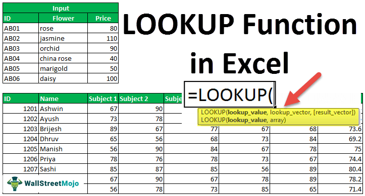
The succeeding table shows a list of flowers, the identifier (ID), and the current price. The output to be retrieved with the help of the LOOKUP function is stated as follows:
a. The price of the flower given its ID
b. The price of the flower given its name
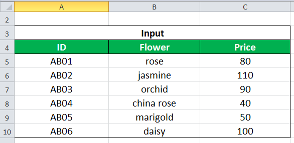
a. We use the following syntax for extracting the price of the flower with its ID.
“=LOOKUP(ID_to_search,A5:A10,C5:C10)”
Since the value to be searched can be supplied as a cell reference, enter E5 in the formula. This is shown in the succeeding image.
“=LOOKUP(E5,A5:A10,C5:C10)”
The formula returns 50.

b. We use the following formula for extracting the price of the flower with its name.
“=LOOKUP(“orchid”,B5:B10,C5:C10)”
The formula returns 90.
Example #2–Vector Form
The following table displays the transaction costs (in dollars) incurred on various dates beginning from January 2009. The output to be retrieved with the help of the LOOKUP function is stated as follows:
a. The cost of the last transaction of 2012
b. The cost of the last transaction of March

a. We use the following formula for extracting information on the last transaction of 2012.
“=LOOKUP(D4,YEAR(A4:A18),B4:B18)”
The “YEAR(A4:A18)” retrieves the year from the dates given in A4:A18. Since D4=2012, the formula returns $40000.

b. We use the following formula for extracting the cost of the last transaction of March.
“=LOOKUP(3,MONTH(A4:A18),B4:B18)”
The “MONTH(A4:A18)” extracts the month from the dates given in A4:A18. The formula returns $110000.
Example #3–Vector Form
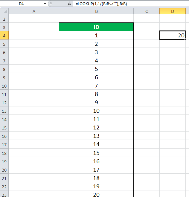
The following table shows a list of IDs in column B. We want to retrieve the last entry of the column with the help of the LOOKUP function. The situations for retrieval are stated as follows:
a. When IDs are listed from 1 to 10
b. When IDs are listed from 1 to 20

a. We use the following formula to extract the last entry of column B.
“=LOOKUP(1,1/(B:B<>””),B:B)”
In the formula, the “lookup_value” is 1, the “lookup_vector” is 1/(B:B<>””), and the “result_vector” is B:B.
The (B:B<>””) forms an array of “true” and “false” where the former means a value is present, while the latter means it is absent. This array is divided by 1 to form another array of “1” and “0” which corresponds to “true” and “false” respectively.
Since the “lookup_value” is 1, the LOOKUP function looks for 1 in the array of “1” and “0.” It matches the “lookup_value” with the last “1” and returns a corresponding match. In this case, the corresponding match is the actual “lookup_value” at the same position, which is 10.
The output of the formula is 10, as shown in the following image.

b. We use the same formula (explained in the preceding section) to extract the last entry of column B.
“=LOOKUP(1,1/(B:B<>””),B:B)”
The formula returns 20, as shown in the following image.
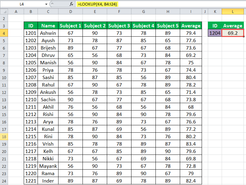
Example #4–Array Form
The following table (B3:I24) shows the roll numbers (ID), names of the students, marks in five subjects, and average marks. We want to retrieve the average marks with the help of the student ID.
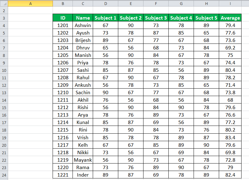
Since the ID to look for is in cell K4, the following formula is used.
“=LOOKUP(K4,B4:I24)”
The formula returns the corresponding average marks of the student Dhruv (ID 1204). The output is 69.2, as shown in the following image.
Applications
The function is used in the following situations:
- To extract the price of an item using its identifier
- To find the location of a book in the library
- To obtain the last transaction cost for a given month or year
- To check the latest price of a product
- To find the last row within a range of numerical or textual data
- To retrieve the last transaction date
Note: The LOOKUP function of Excel is not case-sensitive implying that it treats the uppercase and lowercase letters the same.
Frequently Asked Questions
Define the LOOKUP function of Excel.
The LOOKUP function looks for a value in a single row or column and returns a corresponding value having the same position from another row or column. The look up and the extraction data both should be a one-row or a one-column range.
The LOOKUP function of Excel has two forms which are explained as follows:
• Vector form–The “lookup_value” is searched in the “lookup_vector” and a corresponding match is returned from the “result_vector.” The syntax is stated as follows:
“LOOKUP(lookup_value,lookup_vector,[result_vector])”
The first two arguments are mandatory and the last one is optional.
• Array form–The “lookup_value” is searched in the first row or column of the “array” and a corresponding match is returned from the last row or column of the “array.” The syntax is stated as follows:
“LOOKUP(lookup_value,array)”
Both the arguments are mandatory.
When should the LOOKUP function of Excel be used?
The usage of the general LOOKUP function, the vector, and the array forms is mentioned as follows:
• The general function is used when there is a need to retrieve an associated piece of information from a one-row or a one-column range.
• The vector form is used when there is a need to specify the range from which a corresponding match is to be returned.
• The array form is used when the lookup or search value is in the first row or column and the corresponding match is in the last row or column.
Note: It is recommended to use the VLOOKUP and HLOOKUP as an alternative to the array form.
What is the difference between the LOOKUP, VLOOKUP, and HLOOKUP functions of Excel?
The differences between the three functions are stated as follows:
• The LOOKUP searches for a value in a one-row or one-column range. In contrast, the VLOOKUP and HLOOKUP search for a value in two or more columns or rows respectively.
• The array form of the LOOKUP searches the “lookup_value” according to the dimensions of the array. In comparison, the VLOOKUP and the HLOOKUP search for the “lookup_value” in the first column and the first row respectively.
• The LOOKUP looks for an approximate match while the VLOOKUP and HLOOKUP work for both approximate and exact matches.
• The LOOKUP has cross functionality implying that it is capable of performing both vertical and horizontal lookups. On the other hand, the VLOOKUP and HLOOKUP are limited to only vertical and horizontal lookups respectively.
LOOKUP Excel Video
Recommended Articles
This has been a tutorial to LOOKUP Excel function. Here we discuss how to use LOOKUP formula along with step by step practical examples. You can download the Excel template from the website. You may also go through these useful functions in Excel-
- Power BI VlookupVLOOKUP in Power BI helps the users fetch data from the other tables. Since it is not an inbuilt function, the user needs to replicate it using the DAX function like the LOOKUPVALUE DAX function.read more
- VBA LOOKUPLOOKUP is the function to fetch the data from the main table based on a single lookup value. VBA LOOKUP function doesn’t require a data structure like that. It doesn’t matter whether the result column is to the right or left. It can fetch the data comfortably.read more
- Excel VLOOKUP FormulaThe VLOOKUP excel function searches for a particular value and returns a corresponding match based on a unique identifier. A unique identifier is uniquely associated with all the records of the database. For instance, employee ID, student roll number, customer contact number, seller email address, etc., are unique identifiers.
read more - Degrees Function in ExcelDEGREES function in excel is used to convert the angles mentioned in radians which are determined based on the radius of a circle to degrees. It is one of the mathematical and trigonometric functions inbuilt into Excel to resolve the problem with radians.read more
- Excel TroubleshootingTroubleshooting in Excel helps when we tend to get some errors or unexpected results associated with the formula we use in Excel. read more
Returns a value from a one-row or one-column range
What is the LOOKUP Function?
The LOOKUP Function is categorized under Excel Lookup and Reference functions. The function performs a rough match lookup either in a one-row or one-column range and returns the corresponding value from another one-row or one-column range.
While doing financial analysis, if we wish to compare two rows or columns, we can use the LOOKUP function. It is designed to handle the simplest cases of vertical and horizontal lookup.
The more advanced versions of the LOOKUP function are HLOOKUP and VLOOKUP.
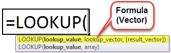
Formula (Vector)
There are two forms of Lookup: Vector and Array.
The vector form of the LOOKUP function will search one row or one column of data for a specified value and then get the data from the same position in another row or column.
The formula for the function is as follows:
=LOOKUP(lookup_value, lookup_vector, [result_vector])
It uses the following arguments:
- Lookup_value (required function) – This is the value that we will be searching. It can be a logical value of TRUE or FALSE, reference to a cell, number, or text.
- Lookup_vector (required function) – This is the one-dimensional data that we wish to search. Remember, we need to sort it in ascending order.
- Result_vector – An optional one-dimensional list of data from which we want to return a value. If supplied, the [result_vector] must be the same length as the lookup_vector. If the [result_vector] is omitted, the result is returned from the lookup_vector.
The array form of LOOKUP looks in the first row or column of an array for the specified value and returns a value from the same position in the last row or column of the array. We need to use this form of LOOKUP when the values that we want to match are in the first row or column of the array.
Formula (Array) LOOKUP Function
= LOOKUP(lookup_value, array)
The arguments are as follows:
- Lookup_value (required argument) – This is a value that we are searching for.
- Array (required argument) – A range of cells that contains text, numbers, or logical values that we want to compare with the lookup_value.
How to use the LOOKUP Function in Excel?
As a worksheet function, the LOOKUP Function can be entered as part of a formula in a cell of a worksheet. To understand the uses of this function, let us consider a few examples:
Example 1
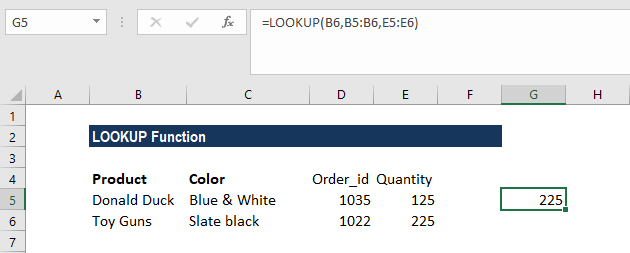
Assume we are given a list of products, color, order_id, and quantity. We want a dashboard where we put the product and then we instantly get the quantity.
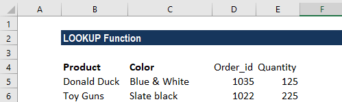
The formula to use will be:
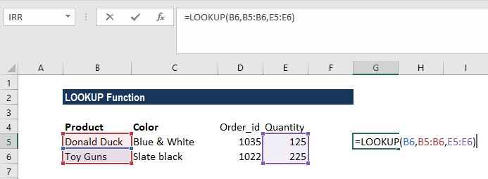
The result we get is:
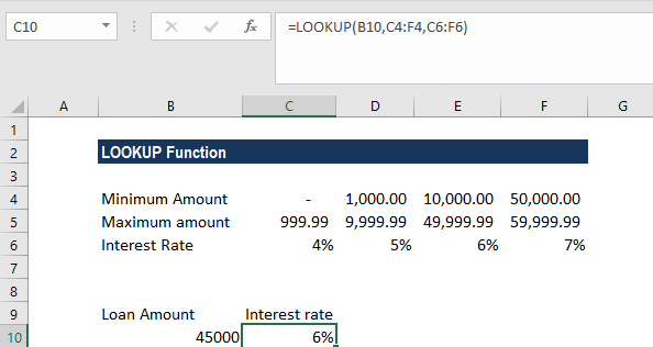
Example 2
Suppose we are in the business of giving loans and we offer different interest rates based on the amount borrowed. We are given the data below:
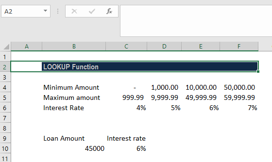
The formula to use will be:
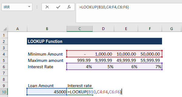
We will get the following result:
Things to remember about the LOOKUP Function:
- #N/A error – Occurs when the Lookup function fails to find the closest match to the supplied lookup_value. This can occur if either:
- The smallest value in the lookup_vector (or first column/row of the array) is greater than the lookup_value provided; or
- The lookup_vector (or first column/row of the array) is not in ascending order.
- #REF! error – Occurs if the formula is attempting to reference cells that are non-existent. This can be caused by either:
- Cells being deleted after the Lookup function has been entered.
- Relative references in the Lookup function that have become invalid when the functions have been copied to other cells.
Click here to download the sample Excel file
Additional resources
Thanks for reading CFI’s guide to important Excel functions! By taking the time to learn and master these functions, you’ll significantly speed up your financial analysis. To learn more, check out these additional CFI resources:
- Excel Functions for Finance
- Advanced Excel Formulas Course
- Advanced Excel Formulas You Must Know
- Excel Shortcuts for PC and Mac
- See all Excel resources
Use the LOOKUP function to look up a value in a one-column or one-row range, and retrieve a value from the same position in another one-column or one-row range. The lookup function has two forms, vector and array. The majority of this article describes the vector form, but the last example below illustrates the array form.
The LOOKUP function accepts three arguments: lookup_value, lookup_vector, and result_vector. The first argument, lookup_value, is the value to look for. The second argument, lookup_vector, is a one-row, or one-column range to search. LOOKUP assumes that lookup_vector is sorted in ascending order. The third argument, result_vector, is a one-row, or one-column range of results. Result_vector is optional. When result_vector is provided, LOOKUP locates a match in the lookup_vector, and returns the corresponding value from result_vector. If result_vector is not provided, LOOKUP returns the value of the match found in lookup_vector.
LOOKUP has default behaviors that make it useful when solving certain problems. For example, LOOKUP can be used to retrieve an approximate-matched value instead of a position and to find the last value in a row or column. LOOKUP assumes that values in lookup_vector are sorted in ascending order and always performs an approximate match. When LOOKUP can’t find a match, it will match the next smallest value.
Example #1 — basic usage
In the example shown above, the formula in cell F5 returns the value of the match found in column B. Note that result_vector is not provided:
=LOOKUP(F4,B5:B9) // returns match in level
The formula in cell F6 returns the corresponding Tier value from column C. Notice in this case, both lookup_vector and result_vector are provided:
=LOOKUP(F4,B5:B9,C5:C9) // returns corresponding tier
In both formulas, LOOKUP automatically performs an approximate match and it is therefore important that lookup_vector is sorted in ascending order.
Example #2 — last non-empty cell
LOOKUP can be used to get the value of the last filled (non-empty) cell in a column. In the screen below, the formula in F6 is:
=LOOKUP(2,1/(B:B<>""),B:B)

Note the use of a full column reference. This is not an intuitive formula, but it works well. The key to understanding this formula is to recognize that the lookup_value of 2 is deliberately larger than any values that will appear in the lookup_vector. Detailed explanation here.
Example #3 — latest price
Similar to the above example, the lookup function can be used to look up the latest price in data sorted in ascending order by date. In the screen below, the formula in G5 is:
=LOOKUP(2,1/(item=F5),price)
where item (B5:B12) and price (D5:D12) are named ranges.

When lookup_value is greater than all values in lookup_array, default behavior is to «fall back» to the previous value. This formula exploits this behavior by creating an array that contains only 1s and errors, then deliberately looking for the value 2, which will never be found. More details here.
Example #4 — array form
The LOOKUP function has an array form as well. In the array configuration, LOOKUP takes just two arguments: the lookup_value, and a single two-dimensional array:
LOOKUP(lookup_value, array) // array form
In the array form, LOOKUP evaluates the array and automatically changes behavior based on the array dimensions. If the array is wider than tall, LOOKUP looks for the lookup value in the first row of the array (like HLOOKUP). If the array is taller than wide (or square), LOOKUP looks for the lookup value in the first column (like VLOOKUP). In either case, LOOKUP returns a value at the same position from the last row or column in the array. The example below shows how the array form works. The formula in F5 is configured to use a vertical array and the formula in F6 is configured to use a horizontal array:
=LOOKUP(E5,B5:C9) // vertical array
=LOOKUP(E6,C11:G12) // horizontal array

The vertical and horizontal arrays contain the same values; only the orientation is different.
Note: Microsoft discourages the use of the array form and suggests VLOOKUP and HLOOKUP as better options.
Notes
- LOOKUP assumes that lookup_vector is sorted in ascending order.
- When lookup_value can’t be found, LOOKUP will match the next smallest value.
- When lookup_value is greater than all values in lookup_vector, LOOKUP matches the last value.
- When lookup_value is less than the first value in lookup_vector, LOOKUP returns #N/A.
- Result_vector must be the same size as lookup_vector.
- LOOKUP is not case-sensitive