What is a function in an excel spreadsheet - Word и Excel - помощь в работе с программами

Home / What is a Function in Excel

What is a Function in Excel

In Excel, a function is a predefined formula that performs a specific calculation by using values a user input as arguments. Every Excel function has a specific purpose, in simple words, it calculates a specific value. Each function has its arguments (the value one needs to input) to get the result value in the cell.

Components

Each function has two major components. In short, each function (except a few) is made up of two following things:

Function Name
Arguments

Let me show you an example. Let’s take a look at the below function which we have inserted in the cell A1.

Now if you look at the formula bar you can understand the structure of the function by splitting it into two parts i.e. name and arguments.

Function Arguments

As I have already mentioned that in a function you need to specify input values to get the desired result. An argument is that value which you need to specify. If you look at the syntax of a function you can see there in each function there is set arguments to specify.

Below are the types of arguments:

Required: A required argument is compulsory for a user to specify and without which a function can’t calculate its result.
Optional: If you skip specifying these arguments it will not stop a function to calculate its result value.
No Arguments: There are few functions (like NOW) where you don’t need to specify any argument.

How to INSERT a Function in Excel

The easiest way to insert a function in a cell in Excel is to type the name of the function you want to insert starting with equals to sign.

Let’s say you want to insert the SUM function:

First of all, you need to type = and the then type SUM.
After that, enter the opening parentheses.
Specify the arguments (refer to a cell or you can directly enter values into the function).
In the end, type closing parentheses and hit enter.

Major Types

Below are the major types:

Text Functions: If you deal with data where you have text, then below are some of the functions which you need to learn to work efficiently.
Date Functions: Dates are one of the major ingredients of data that you use every day, and helps you to analyze your data in a better way.
Time Functions: Just like dates, time is could also be there in data and you can use time functions to deal with data where you have time values.
Logical Functions: Logical functions can help you create some of the most helpful formula in your spreadsheet.
Maths Functions: Excel is all about calculations and analysis, and mathematical functions and you can use these functions to get better in calculations and analysis.
Statistical Functions: One of the best things about Excel is there are a bunch of statistical functions there that you can use to analyze data easily.
Lookup Functions: In Excel, there some specific functions which can help you to look up a value or specific information about a cell or a range of cells.
Information Function: These some specific functions which you can use to get information about the values you supplied.
Financial Functions: These functions can help you calculate some of the common but important financial calculations in an easy way.

About the Author

Puneet is using Excel since his college days. He helped thousands of people to understand the power of the spreadsheets and learn Microsoft Excel. You can ﬁnd him online, tweeting about Excel, on a running track, or sometimes hiking up a mountain.

Источник

Excel for Microsoft 365 Excel 2021 Excel 2019 Excel 2016 Excel 2013 Excel 2010 Excel 2007 More…Less

Functions are predefined formulas that perform calculations by using specific values, called arguments, in a particular order, or structure. Functions can be used to perform simple or complex calculations. You can find all of Excel’s functions on the Formulas tab on the Ribbon:

Excel function syntax

The following example of the ROUND function rounding off a number in cell A10 illustrates a function’s syntax.

1. Structure. The structure of a function begins with an equal sign (=), followed by the function name, an opening parenthesis, the arguments for the function separated by commas, and a closing parenthesis.

2. Function name. For a list of available functions, click a cell and press SHIFT+F3, which will launch the Insert Function dialog.

3. Arguments. Arguments can be numbers, text, logical values such as TRUE or FALSE, arrays, error values such as #N/A, or cell references. The argument you designate must produce a valid value for that argument. Arguments can also be constants, formulas, or other functions.

4. Argument tooltip. A tooltip with the syntax and arguments appears as you type the function. For example, type =ROUND( and the tooltip appears. Tooltips appear only for built-in functions.

Note: You don’t need to type functions in all caps, like =ROUND, as Excel will automatically capitalize the function name for you once you press enter. If you misspell a function name, like =SUME(A1:A10) instead of =SUM(A1:A10), then Excel will return a #NAME? error.
Entering Excel functions

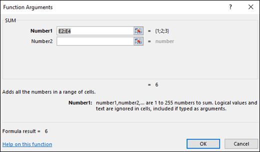
When you create a formula that contains a function, you can use the Insert Function dialog box to help you enter worksheet functions. Once you select a function from the Insert Function dialog Excel will launch a function wizard, which displays the name of the function, each of its arguments, a description of the function and each argument, the current result of the function, and the current result of the entire formula.

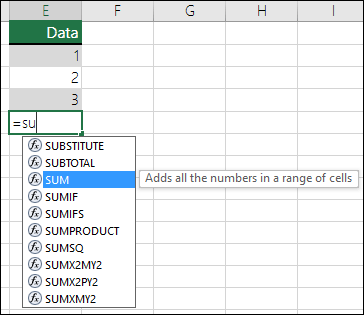
To make it easier to create and edit formulas and minimize typing and syntax errors, use Formula AutoComplete. After you type an = (equal sign) and beginning letters of a function, Excel displays a dynamic drop-down list of valid functions, arguments, and names that match those letters. You can then select one from the drop-down list and Excel will enter it for you.
Nesting Excel functions

In certain cases, you may need to use a function as one of the arguments of another function. For example, the following formula uses a nested AVERAGE function and compares the result with the value 50.

1. The AVERAGE and SUM functions are nested within the IF function.

Valid returns When a nested function is used as an argument, the nested function must return the same type of value that the argument uses. For example, if the argument returns a TRUE or FALSE value, the nested function must return a TRUE or FALSE value. If the function doesn’t, Excel displays a #VALUE! error value.

Nesting level limits A formula can contain up to seven levels of nested functions. When one function (we’ll call this Function B) is used as an argument in another function (we’ll call this Function A), Function B acts as a second-level function. For example, the AVERAGE function and the SUM function are both second-level functions if they are used as arguments of the IF function. A function nested within the nested AVERAGE function is then a third-level function, and so on.

Need more help?

Want more options?

Explore subscription benefits, browse training courses, learn how to secure your device, and more.

Communities help you ask and answer questions, give feedback, and hear from experts with rich knowledge.

Источник

Microsoft Excel’s table structure is a great way to keep organized. But the program is much more than just a series of rows and columns into which you can enter data.

Excel really becomes powerful once you start using functions, which are mathematical formulas that help you quickly and easily make calculations that would be difficult to do by hand.

Functions can do many things to speed up your calculations. For example, you could use functions to take the sum of a row or column of data; find the average of a series of numbers; output the current date; find the number of orders placed by a particular customer within a given period of time; look up the e-mail address of a customer based on his or her name; and much more. It’s all automatic — no manual entry required.

Let’s take a closer look at functions to see how they work.

The structure of a function

Think of a function like a recipe: you put together a series of ingredients, and the recipe spits out something totally new and different (and, in most cases, more useful, or delicious, than the thing that you put in). Like recipes, functions have three key pieces that you should keep track of:

First, there’s the function name. This is just like the recipe name that you would see at the top of one of the pages of your cookbook. It is a unique identifier that tells Excel what we are trying to cook up.
Next, there are arguments. Arguments are just like the ingredients of a recipe. They’re pieces that you put in that will eventually combine to make something bigger.
Finally, there’s the output. The output of a function is just like the output of a recipe — it’s the final product that is ready to be presented to the user (or, in the case of a recipe, eaten).

Writing a function in Excel

When we enter functions into Excel, we use a special character to tell the program that what we are entering is a function and not a normal block of text: the equals sign (=). Whenever Excel sees the = sign at the beginning of the input to a cell, it recognizes that we are about to feed it a function.

The basic structure of a function is as follows:

=FUNCTION_NAME(argument_1, argument_2, argument_3...)
Output: Output

After the = sign, we write the name of the function to tell Excel which recipe we want to use. Then, we use the open parentheses sign (() to tell the program that we’re about to give it a list of arguments.

We then list the arguments to the function, one by one, separated by commas, to tell Excel what ingredients we are using. Note that just like recipes, each function has its own specific number of arguments that it needs to receive. Some just take one argument; others take two or even more.

To finish writing a function, wrap up the list of arguments with the close parentheses sign ()) to tell Excel that you’re done writing the list of ingredients. Then press the Enter key to complete your entry. You’ll see that rather than displaying the text that you entered, Excel shows the output of your completed function.

A practical example

Let’s look at a practical example using the SUM function. This is one of Excel’s most-used recipes — it takes any number of arguments (all of which should be numerical), and spits out the sum of those arguments. The formula for SUM is as follows:

=SUM(number_1, number_2...)

To recap: the name of the function is SUM. The arguments are number_1, number_2, and as many additional numbers as you want to put in (this particular function takes an unlimited number of arguments, just like a recipe that gets better and better as you throw in more ingredients). When you’re done writing the function and press Enter, Excel will show you the output.

Try entering the following into a cell on a blank spreadsheet:

=SUM(3, 7)
Output: 10

Excel outputs 10, because the SUM of 3 and 7 is 10.

Here’s another example with even more arguments:

=SUM(1, 2, 3, 4, 5)
Output: 15

Here, Excel outputs 15, the SUM of 1, 2, 3, 4, and 5.

Infinite arguments and optional arguments

Throughout these pages, we’ll use a couple different types of notation to denote special cases within functions:

First, some functions, like SUM above, have a theoretically infinite number of arguments. For example, you can take the SUM of an infinite number of numerals. In cases like this, we use three dots (…) to denote an infinite number of additional arguments, like so:

=FUNCTION_NAME(argument_1, argument_2, argument_3...)

If a function has a finite number of arguments, you won’t see that … at the end, like this:

=FUNCTION_NAME(argument_1, argument_2)

Finally, some arguments to functions are optional, just like some ingredients of a recipe might be optional. If one or more arguments of a function are optional, we’ll follow them up with an (optional) designator like so:

=FUNCTION_NAME(argument_1, argument_2 (optional))

In most of our function tutorials, we’ll explain why something is optional and how you can use it.

That’s it! Now that you know what a function is, check out our tutorials on some of Excel’s logical functions to get rolling with Excel’s most powerful tool.

Explore the 5 must-learn ‘fundamentals’ of Excel

Getting started with Excel is easy. Sign up for our 5-day mini-course to receive easy-to-follow lessons on using basic spreadsheets.

The basics of rows, columns, and cells…
How to sort and filter data like a pro…
Plus, we’ll reveal why formulas and cell references are so important and how to use them…

Comments

Источник

Lesson 5: Functions

/en/excelformulas/relative-and-absolute-cell-references/content/

Introduction

A function is a predefined formula that performs calculations using specific values in a particular order. All spreadsheet programs include common functions that can be used for quickly finding the sum, average, count, maximum value, and minimum value for a range of cells. In order to use functions correctly, you’ll need to understand the different parts of a function and how to create arguments to calculate values and cell references.

Watch the video below to learn more about using functions in Excel.

The parts of a function

In order to work correctly, a function must be written a specific way, which is called the syntax. The basic syntax for a function is an equals sign (=), the function name (SUM, for example), and one or more arguments. Arguments contain the information you want to calculate. The function in the example below would add the values of the cell range A1:A20.

Working with arguments

Arguments can refer to both individual cells and cell ranges and must be enclosed within parentheses. You can include one argument or multiple arguments, depending on the syntax required for the function.

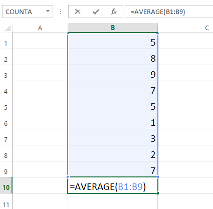
For example, the function =AVERAGE(B1:B9) would calculate the average of the values in the cell range B1:B9. This function contains only one argument.

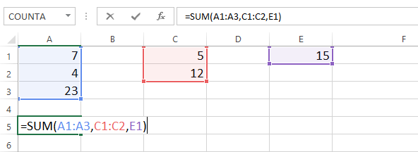
Multiple arguments must be separated by a comma. For example, the function =SUM(A1:A3, C1:C2, E2) will add the values of all cells in the three arguments.

Using functions

There are a variety of functions. Here are some of the most common functions you’ll use:

SUM: This function adds all the values of the cells in the argument.
AVERAGE: This function determines the average of the values included in the argument. It calculates the sum of the cells and then divides that value by the number of cells in the argument.
COUNT: This function counts the number of cells with numerical data in the argument. This function is useful for quickly counting items in a cell range.
MAX: This function determines the highest cell value included in the argument.
MIN: This function determines the lowest cell value included in the argument.

To use a function:

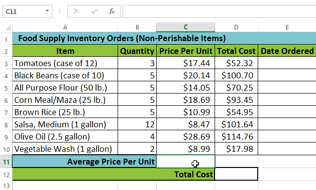
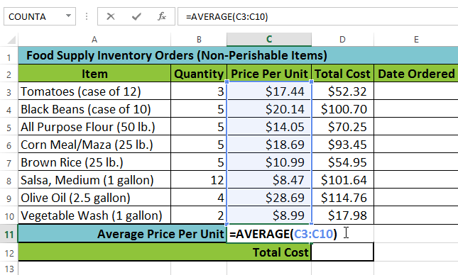
In our example below, we’ll use a basic function to calculate the average price per unit for a list of recently ordered items using the AVERAGE function.

Select the cell that will contain the function. In our example, we’ll select cell C11.
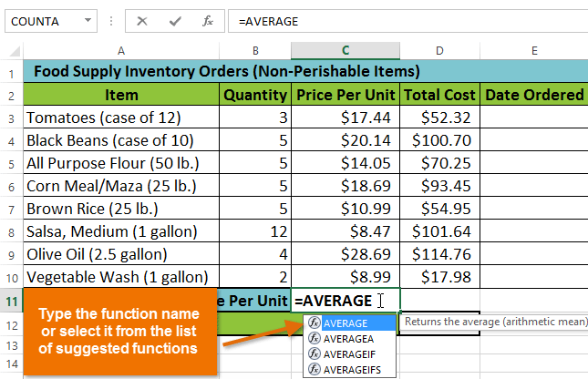
Type the equals sign (=) and enter the desired function name. In our example, we’ll type =AVERAGE.
Enter the cell range for the argument inside parentheses. In our example, we’ll type (C3:C10). This formula will add the values of cells C3:C10 and then divide that value by the total number of cells in the range to determine the average.
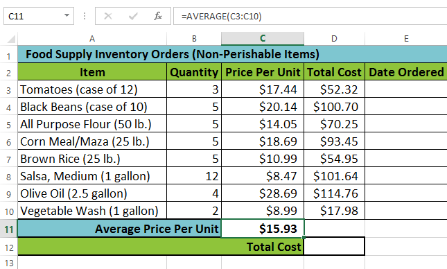
Press Enter on your keyboard. The function will be calculated, and the result will appear in the cell. In our example, the average price per unit of items ordered was $15.93.

Your spreadsheet will not always tell you if your function contains an error, so it’s up to you to check all of your functions. To learn how to do this, check out the Double-Check Your Formulas lesson.

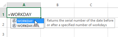
Working with unfamiliar functions

If you want to learn how a function works, you can start typing that function in a blank cell to see what it does.

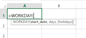
You can then type an open parenthesis to see what kind of arguments it needs.

Understanding nested functions

Whenever a formula contains a function, the function is generally calculated before any other operators, like multiplication and division. That’s because the formula treats the entire function as a single value—before it can use that value in the formula, it needs to run the function. For example, in the formula below, the SUM function will be calculated before division:

Let’s take a look at a more complicated example that uses multiple functions:

=WORKDAY(TODAY(),3)

Here, we have two different functions working together: the WORKDAY function and the TODAY function. These are known as nested functions, since one function is placed, or nested, within the arguments of another. As a rule, the nested function is always calculated first, just like parentheses are performed first in the order of operations. In this example, the TODAY function will be calculated first, since it’s nested within the WORKDAY function.

Other common functions

There are many other functions you can use to quickly calculate different things with your data. Learning how to use other functions will allow you to solve complex problems with your spreadsheets, and we’ll be talking more about them throughout this tutorial. You can also check out our articles below to learn about specific functions:

How to Use Excel’s VLOOKUP Function
How to Count Cells with COUNTA
Use SUMPRODUCT to Calculate Weighted Averages
CONCATENATE: Excel’s Duct Tape
Use the PROPER Function to Capitalize Names in Excel

/en/excelformulas/solving-reallife-problems-in-excel/content/

Источник

Formulas and functions are the building blocks of working with numeric data in Excel. This article introduces you to formulas and functions.

In this article, we will cover the following topics.

What is Formulas in Excel?
Mistakes to avoid when working with formulas in Excel
What is Function in Excel?
The importance of functions
Common functions
Numeric Functions
String functions
Date Time functions
V Lookup function

Tutorials Data

For this tutorial, we will work with the following datasets.

Home supplies budget

S/N	ITEM	QTY	PRICE
1	Mangoes	9	600
2	Oranges	3	1200
3	Tomatoes	1	2500
4	Cooking Oil	5	6500
5	Tonic Water	13	3900

House Building Project Schedule

S/N	ITEM	START DATE	END DATE
1	Survey land	04/02/2015	07/02/2015
2	Lay Foundation	10/02/2015	15/02/2015
3	Roofing	27/02/2015	03/03/2015
4	Painting	09/03/2015	21/03/2015

What is Formulas in Excel?

FORMULAS IN EXCEL is an expression that operates on values in a range of cell addresses and operators. For example, =A1+A2+A3, which finds the sum of the range of values from cell A1 to cell A3. An example of a formula made up of discrete values like =6*3.

=A2 * D2 / 2

HERE,

"=" tells Excel that this is a formula, and it should evaluate it.
"A2" * D2" makes reference to cell addresses A2 and D2 then multiplies the values found in these cell addresses.
"/" is the division arithmetic operator
"2" is a discrete value

Formulas practical exercise

We will work with the sample data for the home budget to calculate the subtotal.

Create a new workbook in Excel
Enter the data shown in the home supplies budget above.
Your worksheet should look as follows.

We will now write the formula that calculates the subtotal

Set the focus to cell E4

Enter the following formula.

=C4*D4

HERE,

"C4*D4" uses the arithmetic operator multiplication (*) to multiply the value of the cell address C4 and D4.

Press enter key

You will get the following result

The following animated image shows you how to auto select cell address and apply the same formula to other rows.

Mistakes to avoid when working with formulas in Excel

Remember the rules of Brackets of Division, Multiplication, Addition, & Subtraction (BODMAS). This means expressions are brackets are evaluated first. For arithmetic operators, the division is evaluated first followed by multiplication then addition and subtraction is the last one to be evaluated. Using this rule, we can rewrite the above formula as =(A2 * D2) / 2. This will ensure that A2 and D2 are first evaluated then divided by two.
Excel spreadsheet formulas usually work with numeric data; you can take advantage of data validation to specify the type of data that should be accepted by a cell i.e. numbers only.
To ensure that you are working with the correct cell addresses referenced in the formulas, you can press F2 on the keyboard. This will highlight the cell addresses used in the formula, and you can cross check to ensure they are the desired cell addresses.
When you are working with many rows, you can use serial numbers for all the rows and have a record count at the bottom of the sheet. You should compare the serial number count with the record total to ensure that your formulas included all the rows.

Check Out
Top 10 Excel Spreadsheet Formulas

What is Function in Excel?

FUNCTION IN EXCEL is a predefined formula that is used for specific values in a particular order. Function is used for quick tasks like finding the sum, count, average, maximum value, and minimum values for a range of cells. For example, cell A3 below contains the SUM function which calculates the sum of the range A1:A2.

SUM for summation of a range of numbers
AVERAGE for calculating the average of a given range of numbers
COUNT for counting the number of items in a given range

The importance of functions

Functions increase user productivity when working with excel. Let’s say you would like to get the grand total for the above home supplies budget. To make it simpler, you can use a formula to get the grand total. Using a formula, you would have to reference the cells E4 through to E8 one by one. You would have to use the following formula.

= E4 + E5 + E6 + E7 + E8

With a function, you would write the above formula as

=SUM (E4:E8)

As you can see from the above function used to get the sum of a range of cells, it is much more efficient to use a function to get the sum than using the formula which will have to reference a lot of cells.

Common functions

Let’s look at some of the most commonly used functions in ms excel formulas. We will start with statistical functions.

S/N	FUNCTION	CATEGORY	DESCRIPTION	USAGE
01	SUM	Math & Trig	Adds all the values in a range of cells	=SUM(E4:E8)
02	MIN	Statistical	Finds the minimum value in a range of cells	=MIN(E4:E8)
03	MAX	Statistical	Finds the maximum value in a range of cells	=MAX(E4:E8)
04	AVERAGE	Statistical	Calculates the average value in a range of cells	=AVERAGE(E4:E8)
05	COUNT	Statistical	Counts the number of cells in a range of cells	=COUNT(E4:E8)
06	LEN	Text	Returns the number of characters in a string text	=LEN(B7)
07	SUMIF	Math & Trig	Adds all the values in a range of cells that meet a specified criteria. =SUMIF(range,criteria,[sum_range])	=SUMIF(D4:D8,”>=1000″,C4:C8)
08	AVERAGEIF	Statistical	Calculates the average value in a range of cells that meet the specified criteria. =AVERAGEIF(range,criteria,[average_range])	=AVERAGEIF(F4:F8,”Yes”,E4:E8)
09	DAYS	Date & Time	Returns the number of days between two dates	=DAYS(D4,C4)
10	NOW	Date & Time	Returns the current system date and time	=NOW()

Numeric Functions

As the name suggests, these functions operate on numeric data. The following table shows some of the common numeric functions.

S/N	FUNCTION	CATEGORY	DESCRIPTION	USAGE
1	ISNUMBER	Information	Returns True if the supplied value is numeric and False if it is not numeric	=ISNUMBER(A3)
2	RAND	Math & Trig	Generates a random number between 0 and 1	=RAND()
3	ROUND	Math & Trig	Rounds off a decimal value to the specified number of decimal points	=ROUND(3.14455,2)
4	MEDIAN	Statistical	Returns the number in the middle of the set of given numbers	=MEDIAN(3,4,5,2,5)
5	PI	Math & Trig	Returns the value of Math Function PI(π)	=PI()
6	POWER	Math & Trig	Returns the result of a number raised to a power. POWER( number, power )	=POWER(2,4)
7	MOD	Math & Trig	Returns the Remainder when you divide two numbers	=MOD(10,3)
8	ROMAN	Math & Trig	Converts a number to roman numerals	=ROMAN(1984)

String functions

These basic excel functions are used to manipulate text data. The following table shows some of the common string functions.

S/N	FUNCTION	CATEGORY	DESCRIPTION	USAGE	COMMENT
1	LEFT	Text	Returns a number of specified characters from the start (left-hand side) of a string	=LEFT(“GURU99”,4)	Left 4 Characters of “GURU99”
2	RIGHT	Text	Returns a number of specified characters from the end (right-hand side) of a string	=RIGHT(“GURU99”,2)	Right 2 Characters of “GURU99”
3	MID	Text	Retrieves a number of characters from the middle of a string from a specified start position and length. =MID (text, start_num, num_chars)	=MID(“GURU99”,2,3)	Retrieving Characters 2 to 5
4	ISTEXT	Information	Returns True if the supplied parameter is Text	=ISTEXT(value)	value – The value to check.
5	FIND	Text	Returns the starting position of a text string within another text string. This function is case-sensitive. =FIND(find_text, within_text, [start_num])	=FIND(“oo”,”Roofing”,1)	Find oo in “Roofing”, Result is 2
6	REPLACE	Text	Replaces part of a string with another specified string. =REPLACE (old_text, start_num, num_chars, new_text)	=REPLACE(“Roofing”,2,2,”xx”)	Replace “oo” with “xx”

Date Time Functions

These functions are used to manipulate date values. The following table shows some of the common date functions

S/N	FUNCTION	CATEGORY	DESCRIPTION	USAGE
1	DATE	Date & Time	Returns the number that represents the date in excel code	=DATE(2015,2,4)
2	DAYS	Date & Time	Find the number of days between two dates	=DAYS(D6,C6)
3	MONTH	Date & Time	Returns the month from a date value	=MONTH(“4/2/2015”)
4	MINUTE	Date & Time	Returns the minutes from a time value	=MINUTE(“12:31”)
5	YEAR	Date & Time	Returns the year from a date value	=YEAR(“04/02/2015”)

VLOOKUP function

The VLOOKUP function is used to perform a vertical look up in the left most column and return a value in the same row from a column that you specify. Let’s explain this in a layman’s language. The home supplies budget has a serial number column that uniquely identifies each item in the budget. Suppose you have the item serial number, and you would like to know the item description, you can use the VLOOKUP function. Here is how the VLOOKUP function would work.

=VLOOKUP (C12, A4:B8, 2, FALSE)

HERE,

"=VLOOKUP" calls the vertical lookup function
"C12" specifies the value to be looked up in the left most column
"A4:B8" specifies the table array with the data
"2" specifies the column number with the row value to be returned by the VLOOKUP function
"FALSE," tells the VLOOKUP function that we are looking for an exact match of the supplied look up value

The animated image below shows this in action

Download the above Excel Code

Summary

Excel allows you to manipulate the data using formulas and/or functions. Functions are generally more productive compared to writing formulas. Functions are also more accurate compared to formulas because the margin of making mistakes is very minimum.

Here is a list of important Excel Formula and Function

SUM function = =SUM(E4:E8)

MIN function = =MIN(E4:E8)

MAX function = =MAX(E4:E8)

AVERAGE function = =AVERAGE(E4:E8)

COUNT function = =COUNT(E4:E8)

DAYS function = =DAYS(D4,C4)

VLOOKUP function = =VLOOKUP (C12, A4:B8, 2, FALSE)

DATE function = =DATE(2020,2,4)

Источник

Most Frequently Used Functions in Excel

List of all Excel Functions

But there are hundreds of other preset formulas offered by Excel:

ABS
ACCRINT
ACCRINTM
ACOS
ACOSH
ACOT
ACOTH
ADDRESS
AGGREGATE
AMORDEGRC
AMORLINC
AND
ARABIC
AREAS
ASC
ASIN
ASINH
ATAN
ATAN2
ATANH
AVEDEV
AVERAGE
AVERAGEA
AVERAGEIF
AVERAGEIFS
BAHTTEXT
BASE
BESSELI
BESSELJ
BESSELK
BESSELY
BETA.DIST
BETA.INV
BETADIST
BETAINV
BIN2DEC
BIN2HEX
BIN2OCT
BINOM.DIST
BINOM.DIST.RANGE
BINOM.INV
BINOMDIST
BITAND
BITLSHIFT
BITOR
BITRSHIFT
BITXOR
CALL
CEILING
CEILING.MATH
CEILING.PRECISE
CELL
CHAR
CHIDIST
CHIINV
CHISQ.DIST
CHISQ.DIST.RT
CHISQ.INV
CHISQ.INV.RT
CHISQ.TEST
CHITEST
CHOOSE
CLEAN
CODE
COLUMN
COLUMNS
COMBIN
COMBINA
COMPLEX
CONCATENATE
CONFIDENCE
CONFIDENCE.NORM
CONFIDENCE.T
CONVERT
CORREL
COS
COSH
COT
COTH
COUNT
COUNTA
COUNTBLANK
COUNTIF
COUNTIFS
COUPDAYBS
COUPDAYS
COUPDAYSNC
COUPNCD
COUPNUM
COUPPCD
COVAR
COVARIANCE.P
COVARIANCE.S
CRITBINOM
CSC
CSCH
CUBEKPIMEMBER
CUBEMEMBER
CUBEMEMBERPROPERTY
CUBERANKEDMEMBER
CUBESET
CUBESETCOUNT
CUBEVALUE
CUMIPMT
CUMPRINC
DATE
DATEVALUE
DAVERAGE
DAY
DAYS
DAYS360
DB
DBCS
DCOUNT
DCOUNTA
DDB
DEC2BIN
DEC2HEX
DEC2OCT
DECIMAL
DEGREES
DELTA
DEVSQ
DGET
DISC
DMAX
DMIN
DOLLAR
DOLLARDE
DOLLARFR
DPRODUCT
DSTDEV
DSTDEVP
DSUM
DURATION
DVAR
DVARP
EDATE
EFFECT
ENCODEURL
EOMONTH
ERF
ERF.PRECISE
ERFC
ERFC.PRECISE
ERROR.TYPE
EUROCONVERT
EVEN
EXACT
EXP
EXPON.DIST
EXPONDIST
F.DIST
F.DIST.RT
F.INV
F.INV.RT
F.TEST
FACT
FACTDOUBLE
FALSE
FDIST
FILTERXML
FIND, FINDB
FINV
FISHER
FISHERINV
FIXED
FLOOR
FLOOR.MATH
FLOOR.PRECISE
FORECAST
FORMULATEXT
FREQUENCY
FTEST
FV
FVSCHEDULE
GAMMA
GAMMA.DIST
GAMMA.INV
GAMMADIST
GAMMAINV
GAMMALN
GAMMALN.PRECISE
GAUSS
GCD
GEOMEAN
GESTEP
GETPIVOTDATA
GROWTH
HARMEAN
HEX2BIN
HEX2DEC
HEX2OCT
HLOOKUP
HOUR
HYPERLINK
HYPGEOM.DIST
HYPGEOMDIST
IF
IFERROR
IFNA
IMABS
IMAGINARY
IMARGUMENT
IMCONJUGATE
IMCOS
IMCOSH
IMCOT
IMCSC
IMCSCH
IMDIV
IMEXP
IMLN
IMLOG10
IMLOG2
IMPOWER
IMPRODUCT
IMREAL
IMSEC
IMSECH
IMSIN
IMSINH
IMSQRT
IMSUB
IMSUM
IMTAN
INDEX
INDIRECT
INFO
INT
INTERCEPT
INTRATE
IPMT
IRR
ISBLANK
ISERR
ISERROR
ISEVEN
ISFORMULA
ISLOGICAL
ISNA
ISNONTEXT
ISNUMBER
ISO.CEILING
ISODD
ISOWEEKNUM
ISPMT
ISREF
ISTEXT
KURT
LARGE
LCM
LEFT, LEFTB
LEN, LENB
LINEST
LN
LOG
LOG10
LOGEST
LOGINV
LOGNORM.DIST
LOGNORM.INV
LOGNORMDIST
LOOKUP
LOWER
MATCH
MAX
MAXA
MDETERM
MDURATION
MEDIAN
MID, MIDB
MIN
MINA
MINUTE
MINVERSE
MIRR
MMULT
MOD
MODE
MODE.MULT
MODE.SNGL
MONTH
MROUND
MULTINOMIAL
MUNIT
N
NA
NEGBINOM.DIST
NEGBINOMDIST
NETWORKDAYS
NETWORKDAYS.INTL
NOMINAL
NORM.DIST
NORM.INV
NORM.S.DIST
NORM.S.INV
NORMDIST
NORMINV
NORMSDIST
NORMSINV
NOT
NOW
NPER
NPV
NUMBERVALUE
OCT2BIN
OCT2DEC
OCT2HEX
ODD
ODDFPRICE
ODDFYIELD
ODDLPRICE
ODDLYIELD
OFFSET
OR
PDURATION
PEARSON
PERCENTILE
PERCENTILE.EXC
PERCENTILE.INC
PERCENTRANK
PERCENTRANK.EXC
PERCENTRANK.INC
PERMUT
PERMUTATIONA
PHI
PHONETIC
PI
PMT
POISSON
POISSON.DIST
POWER
PPMT
PRICE
PRICEDISC
PRICEMAT
PROB
PRODUCT
PROPER
PV
QUARTILE
QUARTILE.EXC
QUARTILE.INC
QUOTIENT
RADIANS
RAND
RANDBETWEEN
RANK
RANK.AVG
RANK.EQ
RATE
RECEIVED
REGISTER.ID
REPLACE, REPLACEB
REPT
RIGHT, RIGHTB
ROMAN
ROUND
ROUNDDOWN
ROUNDUP
ROW
ROWS
RRI
RSQ
RTD
SEARCH, SEARCHB
SEC
SECH
SECOND
SERIESSUM
SHEET
SHEETS
SIGN
SIN
SINH
SKEW
SKEW.P
SLN
SLOPE
SMALL
SQL.REQUEST
SQRT
SQRTPI
STANDARDIZE
STDEV
STDEV.P
STDEV.S
STDEVA
STDEVP
STDEVPA
STEYX
SUBSTITUTE
SUBTOTAL
SUM
SUMIF
SUMIFS
SUMPRODUCT
SUMSQ
SUMX2MY2
SUMX2PY2
SUMXMY2
SYD
T
T.DIST
T.DIST.2T
T.DIST.RT
T.INV
T.INV.2T
T.TEST
TAN
TANH
TBILLEQ
TBILLPRICE
TBILLYIELD
TDIST
TEXT
TIME
TIMEVALUE
TINV
TODAY
TRANSPOSE
TREND
TRIM
TRIMMEAN
TRUE
TRUNC
TTEST
TYPE
UNICHAR
UNICODE
UPPER
VALUE
VAR
VAR.P
VAR.S
VARA
VARP
VARPA
VDB
VLOOKUP
WEBSERVICE
WEEKDAY
WEEKNUM
WEIBULL
WEIBULL.DIST
WORKDAY
WORKDAY.INTL
XIRR
XNPV
XOR
YEAR
YEARFRAC
YIELD
YIELDDISC
YIELDMAT
Z.TEST
ZTEST

The Risk of Vulnerable Functions

Most of the functions mentioned above are rock-solid, but a couple of them we consider vulnerable functions. Some of which are frequently used by many Excel professionals. We suggest you try to avoid using them. Excel offers a range of fine alternatives. PerfectXL helps you discover vulnerable Excel functions in your spreadsheet and helps you find the safe(r) alternatives.

Excel Functions Translated

Blog posts for better Excel use:

The MOST FRUSTRATING feature in Microsoft Excel

The flexibility Excel offers an end user almost guarantees that its approval ratings clearly outpace any ERP. People love how easy it is to get started in Excel, how flexible it is, and how widely known the tool is. While this is all true, the tool can also be frustrating sometimes.

How to tell what changes were made to your Excel model

What do you do when Excel asks you to ‘save your changes’ when you didn’t consciously change anything? Or what if you receive a newer version of a file from a client or coworker, without any explanation of the changes that were made? We’ll help you discover the exact differences between two workbooks, so you can review the changes manually.

Automated visual cell type distinction

PerfectXL Highlighter visually distinguishes different cell types, such as cells with hard coded values, cells with formulas and cells with references. Turn different types of ‘highlights’ on and off to visualize the context of your worksheet and to spot irregularities, like broken formula ranges, at a glance.

Источник

The most frequently used functions in Excel are:

AutoSum;
IF function;
LOOKUP function;
VLOOKUP function;
HLOOKUP function;
MATCH function;
CHOOSE function;
DATE function;

Contents

1 What are the 5 functions in Excel?
2 What are the 10 functions in Excel?
3 What are the 4 major functions of Excel?
4 What are the 20 Excel functions?
5 How many functions are there in Excel?
6 What are the most used functions in Excel?
7 How many types of functions do you know?
8 What is function in Excel with example?
9 What are the six functions of MS Excel?
10 Is there a for function in Excel?
11 What are the 3 common uses for Excel?
12 What are the 12 types of functions?
13 What are the 4 types of functions?
14 What are the 8 types of functions?
15 What are spreadsheet functions?
16 Which is an example of a function?
17 What are the new functions in Excel?
18 How do you use functions in Excel?
19 How do you use the OR function in Excel?
20 What are the types of functions in Excel?

5 Functions of Excel/Sheets That Every Professional Should Know

VLookup Formula.
Concatenate Formula.
Text to Columns.
Remove Duplicates.
Pivot Tables.

What are the 10 functions in Excel?

10 Excel Functions Every Marketer Should Know

Table Formatting. What it does: transforms your data into an interactive database.
Pivot Tables. What it does: summarizes data and finds unique values.
Charting.
COUNTIFS.
SUMIFS.
IF Statements.
CONCATENATE.
VLOOKUP.

What are the 4 major functions of Excel?

To help you get started, here are 5 important Excel functions you should learn today.

The SUM Function. The sum function is the most used function when it comes to computing data on Excel.
The TEXT Function.
The VLOOKUP Function.
The AVERAGE Function.
The CONCATENATE Function.

What are the 20 Excel functions?

Sum. “Sum” is probably the easiest and the most important Excel function at the same time.
Average. Another very important function.
If. Another must-use formula.
Sumif. Sumif is another very useful Excel formula.
Countif. Countif is a very useful function that works like a sumif.
Counta.
Vlookup.
Left, Right, Mid.

How many functions are there in Excel?

Though every Excel feature has a use case, no single person uses every Excel feature themselves. Cut through the 500+ functions, and you’re left with 100 or so truly useful functions and features for the majority of modern knowledge workers.

What are the most used functions in Excel?

SUM functions. Probably the most frequently used function in Excel (or any other spreadsheet program), =SUM does just that: It sums a column, row, or range of numbers—but it doesn’t just sum. It also subtracts, multiplies, divides, and uses any of the comparison operators to return a result of 1 (true) or 0 (false).

How many types of functions do you know?

There are three different forms of representation of functions. The functions need to be represented to showcase the domain values and the range values and the relationship between them.

What is function in Excel with example?

Functions are predefined formulas and are already available in Excel. For example, cell A3 below contains a formula which adds the value of cell A2 to the value of cell A1. For example, cell A3 below contains the SUM function which calculates the sum of the range A1:A2.

What are the six functions of MS Excel?

The six functions are CONCAT, TEXTJOIN, IFS, SWITCH, MAXIFS, and MINIFS. The new chart type is a funnel chart. At least two of these calculation functions are vast improvements over existing functionality.

Is there a for function in Excel?

The FOR… NEXT statement is a built-in function in Excel that is categorized as a Logical Function. It can be used as a VBA function (VBA) in Excel. As a VBA function, you can use this function in macro code that is entered through the Microsoft Visual Basic Editor.

What are the 3 common uses for Excel?

The three most common general uses for spreadsheet software are to create budgets, produce graphs and charts, and for storing and sorting data. Within business spreadsheet software is used to forecast future performance, calculate tax, completing basic payroll, producing charts and calculating revenues.

What are the 12 types of functions?

Terms in this set (12)

Quadratic. f(x)=x^2. D: -∞,∞ R: 0,∞
Reciprocal. f(x)=1/x. D: -∞,0 U 0,∞ R: -∞,0 U 0,∞ Odd.
Exponential. f(x)=e^x. D: -∞,∞ R: 0,∞
Sine. f(x)=SINx. D: -∞,∞ R: -1,1. Odd.
Greatest Integer. f(x)= [[x]] D: -∞,∞ R: {All Integers} Neither.
Absolute Value. f(x)= I x I. D: -∞,∞ R: 0,∞
Linear. f(x)=x. Odd.
Cubic. f(x)=x^3. Odd.

What are the 4 types of functions?

The various types of functions are as follows:

Many to one function.
One to one function.
Onto function.
One and onto function.
Constant function.
Identity function.
Quadratic function.
Polynomial function.

What are the 8 types of functions?

The eight types are linear, power, quadratic, polynomial, rational, exponential, logarithmic, and sinusoidal.

What are spreadsheet functions?

A function is a predefined formula that performs calculations using specific values in a particular order. All spreadsheet programs include common functions that can be used for quickly finding the sum, average, count, maximum value, and minimum value for a range of cells.

Which is an example of a function?

The formula for the area of a circle is an example of a polynomial function.The graph of the function then consists of the points with coordinates (x, y) where y = f(x). For example, the graph of the cubic equation f(x) = x³ − 3x + 2 is shown in the figure.

What are the new functions in Excel?

New functions

CONCAT. This new function is like CONCATENATE, but better.
IFS. Tired of typing complicated, nested IF functions?
MAXIFS. This function returns the largest number in a range, that meets a single or multiple criteria.
MINIFS.
SWITCH.
TEXTJOIN.

How do you use functions in Excel?

Enter a formula that contains a built-in function

Select an empty cell.
Type an equal sign = and then type a function. For example, =SUM for getting the total sales.
Type an opening parenthesis (.
Select the range of cells, and then type a closing parenthesis).
Press Enter to get the result.

How do you use the OR function in Excel?

The OR function is a logical function to test multiple conditions at the same time. OR returns either TRUE or FALSE. For example, to test A1 for either “x” or “y”, use =OR(A1=”x”,A1=”y”).

What are the types of functions in Excel?

Seven Basic Excel Formulas For Your Workflow

SUM. The SUM function. The function will sum up cells that are supplied as multiple arguments.
AVERAGE. The AVERAGE function.
COUNT. The COUNT function.
COUNTA. Like the COUNT function, COUNTA.
IF. The IF function.
TRIM. The TRIM function.
MAX & MIN. The MAX.

Источник

Formulas and functions are the bread and butter of Excel. They drive almost everything interesting and useful you will ever do in a spreadsheet. This article introduces the basic concepts you need to know to be proficient with formulas in Excel. More examples here.

What is a formula?

A formula in Excel is an expression that returns a specific result. For example:

=1+2 // returns 3

=6/3 // returns 2

Note: all formulas in Excel must begin with an equals sign (=).

Cell references

In the examples above, values are «hardcoded». That means results won’t change unless you edit the formula again and change a value manually. Generally, this is considered bad form, because it hides information and makes it harder to maintain a spreadsheet.

Instead, use cell references so values can be changed at any time. In the screen below, C1 contains the following formula:

=A1+A2+A3 // returns 9

Notice because we are using cell references for A1, A2, and A3, these values can be changed at any time and C1 will still show an accurate result.

All formulas return a result

All formulas in Excel return a result, even when the result is an error. Below a formula is used to calculate percent change. The formula returns a correct result in D2 and D3, but returns a #DIV/0! error in D4, because B4 is empty:

There are different ways of handling errors. In this case, you could provide the missing value in B4, or «catch» the error with the IFERROR function and display a more friendly message (or nothing at all).

Copy and paste formulas

The beauty of cell references is that they automatically update when a formula is copied to a new location. This means you don’t need to enter the same basic formula again and again. In the screen below, the formula in E1 has been copied to the clipboard with Control + C:

Below: formula pasted to cell E2 with Control + V. Notice cell references have changed:

Same formula pasted to E3. Cell addresses are updated again:

Relative and absolute references

The cell references above are called relative references. This means the reference is relative to the cell it lives in. The formula in E1 above is:

=B1+C1+D1 // formula in E1

Literally, this means «cell 3 columns left «+ «cell 2 columns left» + «cell 1 column left». That’s why, when the formula is copied down to cell E2, it continues to work in the same way.

Relative references are extremely useful, but there are times when you don’t want a cell reference to change. A cell reference that won’t change when copied is called an absolute reference. To make a reference absolute, use the dollar symbol ($):

=A1 // relative reference
=$A$1 // absolute reference

For example, in the screen below, we want to multiply each value in column D by 10, which is entered in A1. By using an absolute reference for A1, we «lock» that reference so it won’t change when the formula is copied to E2 and E3:

Here are the final formulas in E1, E2, and E3:

=D1*$A$1 // formula in E1
=D2*$A$1 // formula in E2
=D3*$A$1 // formula in E3

Notice the reference to D1 updates when the formula is copied, but the reference to A1 never changes. Now we can easily change the value in A1, and all three formulas recalculate. Below the value in A1 has changed from 10 to 12:

This simple example also shows why it doesn’t make sense to hardcode values into a formula. By storing the value in A1 in one place, and referring to A1 with an absolute reference, the value can be changed at any time and all associated formulas will update instantly.

Tip: you can toggle between relative and absolute syntax with the F4 key.

How to enter a formula

To enter a formula:

Select a cell
Enter an equals sign (=)
Type the formula, and press enter.

Instead of typing cell references, you can point and click, as seen below. Note references are color-coded:

All formulas in Excel must begin with an equals sign (=). No equals sign, no formula:

How to change a formula

To edit a formula, you have 3 options:

Select the cell, edit in the formula bar
Double-click the cell, edit directly
Select the cell, press F2, edit directly

No matter which option you use, press Enter to confirm changes when done. If you want to cancel, and leave the formula unchanged, click the Escape key.

Video: 20 tips for entering formulas

What is a function?

Working in Excel, you will hear the words «formula» and «function» used frequently, sometimes interchangeably. They are closely related, but not exactly the same. Technically, a formula is any expression that begins with an equals sign (=).

A function, on the other hand, is a formula with a special name and purpose. In most cases, functions have names that reflect their intended use. For example, you probably know the SUM function already, which returns the sum of given references:

=SUM(1,2,3) // returns 6
=SUM(A1:A3) // returns A1+A2+A3

The AVERAGE function, as you would expect, returns the average of given references:

=AVERAGE(1,2,3) // returns 2

And the MIN and MAX functions return minimum and maximum values, respectively:

=MIN(1,2,3) // returns 1
=MAX(1,2,3) // returns 3

Excel contains hundreds of specific functions. To get started, see 101 Key Excel functions.

Function arguments

Most functions require inputs to return a result. These inputs are called «arguments». A function’s arguments appear after the function name, inside parentheses, separated by commas. All functions require a matching opening and closing parentheses (). The pattern looks like this:

=FUNCTIONNAME(argument1,argument2,argument3)

For example, the COUNTIF function counts cells that meet criteria, and takes two arguments, range and criteria:

=COUNTIF(range,criteria) // two arguments

In the screen below, range is A1:A5 and criteria is «red». The formula in C1 is:

=COUNTIF(A1:A5,"red") // returns 2

Video: How to use the COUNTIF function

Not all arguments are required. Arguments shown in square brackets are optional. For example, the YEARFRAC function returns fractional number of years between a start date and end date and takes 3 arguments:

=YEARFRAC(start_date,end_date,[basis])

Start_date and end_date are required arguments, basis is an optional argument. See below for an example of how to use YEARFRAC to calculate current age based on birthdate.

How to enter a function

If you know the name of the function, just start typing. Here are the steps:

1. Enter equals sign (=) and start typing. Excel will make a list of matching functions based as you type:

When you see the function you want in the list, use the arrow keys to select (or just keep typing).

2. Type the Tab key to accept a function. Excel will complete the function:

3. Fill in required arguments:

4. Press Enter to confirm formula:

Combining functions (nesting)

Many Excel formulas use more than one function, and functions can be «nested» inside each other. For example, below we have a birthdate in B1 and we want to calculate current age in B2:

The YEARFRAC function will calculate years with a start date and end date:

We can use B1 for start date, then use the TODAY function to supply the end date:

When we press Enter to confirm, we get current age based on today’s date:

=YEARFRAC(B1,TODAY())

Notice we are using the TODAY function to feed an end date to the YEARFRAC function. In other words, the TODAY function can be nested inside the YEARFRAC function to provide the end date argument. We can take the formula one step further and use the INT function to chop off the decimal value:

=INT(YEARFRAC(B1,TODAY()))

Here, the original YEARFRAC formula returns 20.4 to the INT function, and the INT function returns a final result of 20.

Notes:

The current date in images above is February 22, 2019.
Nested IF functions are a classic example of nesting functions.
The TODAY function is a rare Excel function with no required arguments.

Key takeaway: The output of any formula or function can be fed directly into another formula or function.

Math Operators

The table below shows the standard math operators available in Excel:

Symbol	Operation	Example
+	Addition	=2+3=5
—	Subtraction	=9-2=7
*	Multiplication	=6*7=42
/	Division	=9/3=3
^	Exponentiation	=4^2=16
()	Parentheses	=(2+4)/3=2

Logical operators

Logical operators provide support for comparisons such as «greater than», «less than», etc. The logical operators available in Excel are shown in the table below:

Operator	Meaning	Example
=	Equal to	=A1=10
<>	Not equal to	=A1<>10
>	Greater than	=A1>100
<	Less than	=A1<100
>=	Greater than or equal to	=A1>=75
<=	Less than or equal to	=A1<=0

Video: How to build logical formulas

Order of operations

When solving a formula, Excel follows a sequence called «order of operations». First, any expressions in parentheses are evaluated. Next Excel will solve for any exponents. After exponents, Excel will perform multiplication and division, then addition and subtraction. If the formula involves concatenation, this will happen after standard math operations. Finally, Excel will evaluate logical operators, if present.

Parentheses
Exponents
Multiplication and Division
Addition and Subtraction
Concatenation
Logical operators

Tip: you can use the Evaluate feature to watch Excel solve formulas step-by-step.

Convert formulas to values

Sometimes you want to get rid of formulas, and leave only values in their place. The easiest way to do this in Excel is to copy the formula, then paste, using Paste Special > Values. This overwrites the formulas with the values they return. You can use a keyboard shortcut for pasting values, or use the Paste menu on the Home tab on the ribbon.

Video: Paste Special Shortcuts

What’s next?

Below are guides to help you learn more about Excel’s formulas and functions. We also offer online video training.

29 tips for working with formulas and functions (video version here)
500 formula examples with full explanations
101 important Excel functions
Guide to all Excel functions (work in progress)
Excel formula errors (examples and fixes)
Formula criteria — 50 examples
Formulas for conditional formatting
How to use F9 to debug a formula (video)
Excel formula errors and fixes (video)

Источник

15 Most Common Excel Functions You Must Know + How to Use Them

Microsoft Excel is one of the most well-known computer applications. It has changed the way people and companies work with data.

Thus, learning Excel can help with both your career and your personal needs.

Excel runs using functions and there are roughly 500 of them! These range from basic arithmetic to complex statistics.

Most Excel users will only ever use about 100 of these functions

If you’re a new Excel user, this sheer quantity can be quite daunting.

So we are here to help you! 🤝

We have rounded up 15 of the most common and useful Excel functions that you need to learn. We also prepared a practice workbook for you to follow along with the examples. Download it here.

Let’s get started!

What are Excel functions?

Excel is used to calculate and manipulate numbers and text. To do this, you use formulas!

Formulas are expressions that tell Excel what you want to do with the data. They begin with the equal symbol (=) followed by a combination of operators and functions.

What are operators?

These are symbols that specify the type of calculation you want to perform on the elements of a formula.

For example, to add two numbers, you can type “=1+1” into a cell. Once you hit Enter, Excel will run the formula and return the result which is 2.

Here are some examples of common operators:

An arithmetic calculation return a number, comparisons return a Boolean or logical value i.e. TRUE or FALSE

Excel automatically treats cell contents that start with (=) as formulas. This also applies when you begin a cell with the plus (+) or minus (-) symbols.

You can bypass this by adding a leading apostrophe (‘). This is how you can show formulas as text like in the table above.

Order of operation and using parentheses in Excel formulas

Generally, Excel follows PEMDAS when calculating formulas. PEMDAS means parentheses first, then exponents, then multiplication and division, then addition and subtraction.

Adding parentheses changes how a formula calculates

What are functions?

These are predefined processes in Excel. Each function in Excel has a unique name and specific input(s). The function takes these inputs and performs the corresponding calculation.

The inputs or arguments of an Excel function are always enclosed in parentheses.

For example, this is the syntax for the MAX function:

=MAX(number1, [number2], …)

The list of numbers where you want to find the maximum value is placed inside the parentheses.

MAX returns the maximum value from a group of numbers, the function MIN does the same for the minimum value

Using a cell or a range as input

As you learn more about Excel, you’ll find that Excel formulas rarely consist of individual numbers only like in the formula “=1+1”.

Often, you need to reference a cell or a range(group of cells) as the input of your Excel function

Thus, referencing cells is important in Excel and you can learn more by clicking here.

Alright! You’ve just learned how a function in Excel works.

Let’s dive right into the list! 🤿

We will start with basic Excel functions and then move on to more advanced functions.

Basic Math Functions (Beginner Level ★☆☆)

1. SUM

This is the first function in Excel that most new users need. As the name implies, the SUM function adds up all the values in a specified group of cells or range.

Syntax: =SUM(number1, [number2], …)

Try it out in the practice workbook.

If you want to get the total quiz score for each student, you can use the SUM function. In this case, the input range will be all four quiz scores for each student.

1. Type this formula into cell F2:

=SUM(B2:E2)

You can also type “=SUM(B2,C2,D2,E2)” but “=SUM(B2:E2)” is much simpler.

You can also drag the input selection(blue box) over to your desired range

2. Press Enter. Excel then evaluates the formula and the cell returns the number for the total which is 360.

3. Copy this for the rest of the students or drag down the fill handle.

The fill handle is the small green square at bottom right of the cell

Notice that the SUM function ignores the cells containing text. (“X” meaning the student was unable to take the quiz)

Most of the basic math functions in Excel ignore non-numeric values such as text, date, and time.

2. COUNT

Next up is the COUNT function. It returns the number of cells containing numeric values within the input range.

Syntax: =COUNT(value1, [value2], …)

1. To get the number of quizzes taken by each student, use this formula in cell G2:

=COUNT(B2:E2)

2. Hit Enter and fill in the rows below.

If you would like to include non-numeric values in the count, you can use the COUNTA function. To count the number of blank cells, you can use the COUNTBLANK function.

Learn more about the COUNT function and its variants here.

3. AVERAGE

The average of a list of numbers is just the total divided by how many numbers there are in that list.

This is easy enough to calculate the quiz scores. You already have the SUM and the COUNT of quizzes for each student.

But, it gets even easier using the AVERAGE function in Excel.

Syntax: =AVERAGE (value1, [value2], …)

1. Type this into cell H2:

=AVERAGE(B2:E2)

2. Hit Enter and fill in the rows below.

Use Cell Formatting to change the number of decimals displayed

You can double-check the results using the SUM and COUNT functions earlier.

Logical Functions (Intermediate Level – ★★☆)

Let’s raise the difficulty level a little bit.

A logical function in Excel allows you to make comparisons and use the results to change how a formula calculates.

4. IF

The IF function is a very popular function in Excel and it is actually quite easy to learn.

Syntax: =IF(logical_test, value_if_true, [value_if_false])

This function checks if a logical test is either TRUE or FALSE. It then returns the specified value based on the result.

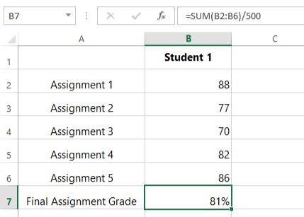
Using the average score of each student, try to assign PASS or FAIL grades. Assume that the passing score for this class is 60.

1. Begin the formula in cell C2 with “=IF(“

The logical_test is to check if the average score in Column B is greater than or equal to (>=) the passing score of 60.

2. So, the formula becomes:

=IF(B2>=60,

If the comparison returns TRUE, then the formula should return the text “PASS”. Thus, the value_if_true argument should be “PASS”.

And if it returns FALSE, then the value_if_false argument should be “FAIL”.

3. Thus, the formula becomes:

=IF(B2>=60,”PASS”,”FAIL”)

4. Hit Enter and fill in the rows below.

Luckily everyone in this class has passed

What if you needed to assign grades according to a scale instead of just “PASS” and “FAIL”?

For that, you have to use multiple criteria or logical tests. While this is possible using nested IF functions, it can get messy very quickly. Instead, you can use the IFS function.

5. IFS function

The IFS function was introduced in Excel 2016 to replace nested IF functions.

This function works by evaluating the first logical test or criteria. It returns the corresponding value if it is TRUE. But if it is FALSE, the function proceeds to evaluate the second criteria, and so on.

📖 In other words, the IFS function outputs the value that corresponds to the first specified criteria that is true.

Syntax: =IFS(logical_test1, value_if_true1, [logical_test2], [value_if_true2],..)

Use the grading table on the right as reference

1. First, the formula should check if the average score (column B) is above or equal to 90. If yes, it should return “A”.

=IFS(B2>=90,”A”,

2. If not, it should then check if the average score is greater than or equal to 80. If yes, it should return “B”. If you do this up to grade D, the formula becomes:

=IFS(B2>=90,”A”,B2>=80,”B”,B2>=70,”C”,B2>=60,”D”,

3. For the last grade “F”, put “TRUE” for the logical test.

The IFS function will only evaluate the last specified criteria if all of the previous logical values were FALSE. Thus, you can set the last criteria to always be TRUE thus making it a “catch all” statement.

The final formula is then:

=IFS(B2>=90,”A”,B2>=80,”B”,B2>=70,”C”,B2>=60,”D”,TRUE,”F”)

PRO-TIP:

You can use absolute cell references and a reference table when working with long formulas.

That way, you don’t have to revisit all of the arguments in the formula if you need to change some values.

For example, using the table and formula shown below, you can easily change the grading scale in use.

=IFS(B2>=$H$2,$F$2,B2>=$H$3,$F$3,B2>
=$H$4,$F$4,B2>=$H$5,$F$5,TRUE,$F$6)

The dollar sign ($) in a formula denotes an absolute cell reference, ex: $F$2

Text Functions (Intermediate Level – ★★☆)

In this next section, you will see how Excel can also be used to manipulate text.

In the “Class List” worksheet of the practice workbook, the full name of each student is listed in Column A. Your goal is to rearrange these from “first name last name” to “last name_first name” in Column F.

The finished table will let users sort using both first and last name

To do this, you first have to extract the first name and the last name from Column A.

6. FIND

The names are separated by a space character ” “. So, you have to identify the position of the space within each text string in Column A.

The FIND function in Excel returns the number or position of a specified character or substring within another text string.

Syntax: =FIND(find_text, within_text, [start_num])

To get the position of the space ” “, type this formula:

=FIND(” “,A2)

You will use these results to extract the first name later

Next, take a look at the LEN function.

7. LEN

This function returns the number of characters in a text string.

Syntax: =LEN(text)

To get the number of characters in each student’s name:

=LEN(A2)

You will use the LEN results to extract the last name later

Now you can move on to extracting the first and last name using the MID function in Excel.

8. MID

This function extracts a given number of characters from the middle of a text string.

Syntax: = MID(text, start_num, num_chars)

It is one of three text functions that are used to extract text. The other two are LEFT and RIGHT which extract text from the start and end of a text string respectively.

The first name starts at the very first character of the text string. So, you extract starting from position 1. Then the length of the first name is given by the position of the space character minus 1.

So, the formula to extract the first name or first word from a text string is:

=MID(A2,1,B2-1)

Or, you can express it directly using the FIND formula earlier.

=MID(A2,1,FIND(” “,A2)-1)

This formula works for any text string you need to grab the first word from

For the last name, you can extract it starting from the position of the space character plus 1. Its length is just the length of the entire text string minus the position of the space character.

=MID(A2,B2+1,C2-B2)

Or, using the FIND and LEN formulas earlier:

=MID(A2,FIND(” “,A2)+1,LEN(A2)-FIND(” “,A2))

The space character's position number raised by 1 gives the starting position of the last name

Now you can combine the last name and the first name in the desired order using the CONCAT function.

9. CONCAT

Like IFS, CONCAT is another newly introduced function in Excel 2016. It replaced the old CONCATENATE function.

Syntax: =CONCAT(text1, [text2],…)

Combine the last name and the first name with a comma and space character “, ” in between.

=CONCAT(E2,”, “,D2)

CONCAT also converts input numbers to text

PRO-TIP:

In the above example, you used helper columns for FIND, LEN, and MID to help build the final formula and visualize how it works.

In real-world applications, you can use a single long formula to get the results like this:

=CONCAT(MID(A2,FIND(” “,A2)+1,LEN(A2)
-FIND(” “,A2)),”, “,MID(A2,1,FIND(” “,A2)-1))

Helper columns are useful in building and testing long formulas

Lookup and Reference Functions (Advanced Level – ★★★)

In this final section, we will focus on functions that allow you to look for specific data points and refer to them.

Take a look at the “Schedule” worksheet.

You will find the schedule and seating plan for the next four quizzes

10. COLUMN

The COLUMN function in Excel returns the column number of a given cell.

Syntax: =COLUMN([reference])

Let’s try to assign specific dates for each quiz. For example, you may want the quizzes to be held every Monday. This means that the first quiz date should be offset by 1 week or 7 days for each succeeding quiz date.

You can use the column number to multiply the 7 days offset for each week like this:

=$B$2+(COLUMN()-2)*7

The start date, Oct 3, is highlighted in green and its column number, 2, is subtracted from the formula

Two (2) is subtracted from the column number so that the sequence starts at 1.

You can also get this result using the much simpler “=B2+7” since you are only adding a fixed number of days to each date. 🤔

But, using the COLUMN function, you can create complex patterns.

Take this pattern for example:

The quizzes are still held every Monday. But every third week, they are held on Wednesday instead.

Here is the formula for this pattern:

=$B$2+(COLUMN()-2)*7+IF(MOD(COLUMN()-1,3)=0,2,0)

The formula is a bit long so here is a breakdown of how it works

The MOD function in Excel returns the remainder after a number is divided by a given divisor. It’s part of the Math & Trig group of functions.

This group includes other fun functions such as ABS which returns the absolute value of a number and ROUND which rounds a number to a specified number of digits.

Learn more about the function groups towards the end of this article!

Kasper Langmann, Microsoft Office Specialist

11. ROW

Next, take a look at the ROW function. It works exactly like COLUMN but it returns the row number instead.

Syntax: =ROW([reference])

In this next example, you will assign the seating plans. You can try different seating arrangements using the ROW function.

Assume R1C1 is the seat closest to the teacher’s desk.

1. You can have the students seated one seat after another and in two columns:

=CONCAT(“R”,MOD(ROW()-6,3)*2+1,”C”,INT((ROW()-6)/3)*2+1)

The INT function in Excel rounds a number down to the nearest integer

2. Or they can sit in rows of 3 and columns of 2

=CONCAT(“R”,MOD(ROW()-6,2)*2+1,”C”,INT((ROW()-6)/2)*2+1)

You can modify the values in the formula to change the seating pattern

3. You can also sit them in the farthest rows:

=CONCAT(“R”,MOD(ROW()-6,2)*4+1,”C”,INT((ROW()-6)/2)*2+1)

In this seating plan, students have the most distance from the front and back

4. Or in the farthest columns:

=CONCAT(“R”,MOD(ROW()-6,3)*2+1,”C”,INT((ROW()-6)/3)*4+1)

In this seating plan, students have the most distance from the sides

Manually creating seating patterns for small sets like this one is easy. But a formula like those shown above definitely helps especially for larger sets like 50, 100, or even more.

The COLUMN and ROW functions are rarely used on their own. Like IF and IFS, you use them with other functions to change how the formula is calculated.

12. MATCH

Now, open up the “Lookup” worksheet.

In the next few examples, you will create a search feature that allows students to look up their names. They can then see their scores from past quizzes and their assigned seats for the next quizzes.

To start, you will use the MATCH function. It searches for a specified item within a given range of cells. It then returns the relative position of the first match.

Syntax: =MATCH(lookup_value, lookup_array, [match_type])

The lookup_value is the item you want to search for. So, set this to cell B2.
The lookup_array is the range or table array where you want to search. Use F2:F7 from the “Class List” worksheet.
For the match_type, set this to zero so that the function searches for an exact match. (Learn more about MATCH and the different match types in this article)

The formula then becomes:

=MATCH(B2,’Class List’!F2:F7,0)

Students can now search for their names and the function returns the relative position in the Class List table

However, it only works correctly if the name is entered exactly as it is written in Column F of the Class List.

To fix this, you can use the asterisk “*” wildcard character so that searching for either first or last name works.

You can also enclose the formula in an IFNA function. This way, if the formula cannot find the given name in the table, it will return a phrase like “No result found”.

You will later use the resulting Row to retrieve the first and last name

13. INDEX

The INDEX function retrieves a value from a given table array based on the provided row and column numbers.

Syntax: =INDEX (array, row_num, [col_num])

Similar to the MATCH example, you need to specify where the range or array lookup is.

Use D2:E7 from Class List as the table array

For row_num, you can use the earlier MATCH result at Cell B5. Then for col_num, use 1 for the First Name:

=INDEX(‘Class List’!D2:E7,B5,1)

And set col_num to 2 for the Last Name.

=INDEX(‘Class List’!D2:E7,B5,2)

Just like that, you have a working search 🔍 formula!

This is just a small example of the countless possibilities using the INDEX and MATCH combination. Click here for more examples!

14. VLOOKUP

The VLOOKUP function in Excel works similarly to the INDEX and MATCH combination. It is faster to set up but it is less versatile. VLOOKUP also only works if your lookup array is at the leftmost of the reference table.

Syntax: =VLOOKUP (lookup_value, table_array, col_index_num, [range_lookup])

This time, you will use the First Name result (cell B6) as the lookup_value. Use this and VLOOKUP to retrieve the given student’s scores from the “Quiz Scores” worksheet.

=VLOOKUP($B$6,’Quiz Scores’!$A$2:$E$7,COLUMN(),FALSE)

For the seat assignment, use the Last Name result followed by the asterisk wild character.

=VLOOKUP($B$7&”*”,Schedule!$A$6:$E$11,COLUMN(),FALSE)

15. INDIRECT

The last function that you will be learning about today is also one of the most powerful in Excel.

INDIRECT allows you to specify cell references using text strings.

SYNTAX: =INDIRECT(ref_text, [a1])

For example, instead of typing “=A1”, you can type “=INDIRECT(“A”&1). This means you can dynamically change references.

Let’s take the INDEX & MATCH formula you used to retrieve the Last Name. You can get the same result using this formula:

=INDIRECT(“‘Class List’!”&”E”&(B5+1))

This is a simple example and definitely doesn't do justice to how powerful INDIRECT really is

The INDIRECT function opens up so many possibilities with dynamic references in Excel. I highly this article for an in-depth tutorial on INDIRECT.

That’s it – Now what?

As you have just learned, Excel offers so many different functions to choose from. Luckily, Excel has brought them all together in the Formulas tab.

The functions are categorized into groups such as Math & Trigonometry, Text, & Date and Time

You can look for an Excel function using search keywords or you can also select from the categorical dropdowns.

For example, click on the Financial group to find functions that can help you calculate items like net present value, future value, cumulative interest paid, cumulative principal paid, etc.

NOMINAL returns the annual nominal interest rate

You can also click on More Functions which opens up even more possibilities for advanced Excel formulas.

For example, the Statistical group is useful if you need to calculate a statistical value. This includes functions for maximum value, minimum value, forecast value, gamma function value, etc. You can insert a cumulative distribution function and other useful tools for data analysis.

NORM.DIST can be used either as a cumulative distribution function or as a probability density function

Learn how to use these formulas and more by signing up for my free online Excel course.

We will help you make the most out of your Excel experience! 📈

Other relevant resources

If you enjoyed this article, you can visit my YouTube channel for more in-depth tutorials and other fun stuff!

Did you know that the Flash Fill feature can help speed up your work by automatically filling a repetitive pattern Excel detects from your data? Learn more here.

Thanks for reading! 😄

Kasper Langmann2023-02-23T11:47:15+00:00

Page load link

Источник