
Overview of formulas in Excel
Get started on how to create formulas and use built-in functions to perform calculations and solve problems.

Important: The calculated results of formulas and some Excel worksheet functions may differ slightly between a Windows PC using x86 or x86-64 architecture and a Windows RT PC using ARM architecture. Learn more about the differences.
Important: In this article we discuss XLOOKUP and VLOOKUP, which are similar. Try using the new XLOOKUP function, an improved version of VLOOKUP that works in any direction and returns exact matches by default, making it easier and more convenient to use than its predecessor.
Create a formula that refers to values in other cells
-
Select a cell.
-
Type the equal sign =.
Note: Formulas in Excel always begin with the equal sign.
-
Select a cell or type its address in the selected cell.

-
Enter an operator. For example, – for subtraction.
-
Select the next cell, or type its address in the selected cell.
-
Press Enter. The result of the calculation appears in the cell with the formula.


See a formula
-
When a formula is entered into a cell, it also appears in the Formula bar.
-
To see a formula, select a cell, and it will appear in the formula bar.


Enter a formula that contains a built-in function
-
Select an empty cell.
-
Type an equal sign = and then type a function. For example, =SUM for getting the total sales.
-
Type an opening parenthesis (.
-
Select the range of cells, and then type a closing parenthesis).
-
Press Enter to get the result.

Download our Formulas tutorial workbook
We’ve put together a Get started with Formulas workbook that you can download. If you’re new to Excel, or even if you have some experience with it, you can walk through Excel’s most common formulas in this tour. With real-world examples and helpful visuals, you’ll be able to Sum, Count, Average, and Vlookup like a pro.
Formulas in-depth
You can browse through the individual sections below to learn more about specific formula elements.
A formula can also contain any or all of the following: functions, references, operators, and constants.
Parts of a formula

1. Functions: The PI() function returns the value of pi: 3.142…
2. References: A2 returns the value in cell A2.
3. Constants: Numbers or text values entered directly into a formula, such as 2.
4. Operators: The ^ (caret) operator raises a number to a power, and the * (asterisk) operator multiplies numbers.
A constant is a value that is not calculated; it always stays the same. For example, the date 10/9/2008, the number 210, and the text «Quarterly Earnings» are all constants. An expression or a value resulting from an expression is not a constant. If you use constants in a formula instead of references to cells (for example, =30+70+110), the result changes only if you modify the formula. In general, it’s best to place constants in individual cells where they can be easily changed if needed, then reference those cells in formulas.
A reference identifies a cell or a range of cells on a worksheet, and tells Excel where to look for the values or data you want to use in a formula. You can use references to use data contained in different parts of a worksheet in one formula or use the value from one cell in several formulas. You can also refer to cells on other sheets in the same workbook, and to other workbooks. References to cells in other workbooks are called links or external references.
-
The A1 reference style
By default, Excel uses the A1 reference style, which refers to columns with letters (A through XFD, for a total of 16,384 columns) and refers to rows with numbers (1 through 1,048,576). These letters and numbers are called row and column headings. To refer to a cell, enter the column letter followed by the row number. For example, B2 refers to the cell at the intersection of column B and row 2.
To refer to
Use
The cell in column A and row 10
A10
The range of cells in column A and rows 10 through 20
A10:A20
The range of cells in row 15 and columns B through E
B15:E15
All cells in row 5
5:5
All cells in rows 5 through 10
5:10
All cells in column H
H:H
All cells in columns H through J
H:J
The range of cells in columns A through E and rows 10 through 20
A10:E20
-
Making a reference to a cell or a range of cells on another worksheet in the same workbook
In the following example, the AVERAGE function calculates the average value for the range B1:B10 on the worksheet named Marketing in the same workbook.
1. Refers to the worksheet named Marketing
2. Refers to the range of cells from B1 to B10
3. The exclamation point (!) Separates the worksheet reference from the cell range reference
Note: If the referenced worksheet has spaces or numbers in it, then you need to add apostrophes (‘) before and after the worksheet name, like =’123′!A1 or =’January Revenue’!A1.
-
The difference between absolute, relative and mixed references
-
Relative references A relative cell reference in a formula, such as A1, is based on the relative position of the cell that contains the formula and the cell the reference refers to. If the position of the cell that contains the formula changes, the reference is changed. If you copy or fill the formula across rows or down columns, the reference automatically adjusts. By default, new formulas use relative references. For example, if you copy or fill a relative reference in cell B2 to cell B3, it automatically adjusts from =A1 to =A2.
Copied formula with relative reference
-
Absolute references An absolute cell reference in a formula, such as $A$1, always refer to a cell in a specific location. If the position of the cell that contains the formula changes, the absolute reference remains the same. If you copy or fill the formula across rows or down columns, the absolute reference does not adjust. By default, new formulas use relative references, so you may need to switch them to absolute references. For example, if you copy or fill an absolute reference in cell B2 to cell B3, it stays the same in both cells: =$A$1.
Copied formula with absolute reference
-
Mixed references A mixed reference has either an absolute column and relative row, or absolute row and relative column. An absolute column reference takes the form $A1, $B1, and so on. An absolute row reference takes the form A$1, B$1, and so on. If the position of the cell that contains the formula changes, the relative reference is changed, and the absolute reference does not change. If you copy or fill the formula across rows or down columns, the relative reference automatically adjusts, and the absolute reference does not adjust. For example, if you copy or fill a mixed reference from cell A2 to B3, it adjusts from =A$1 to =B$1.
Copied formula with mixed reference
-
-
The 3-D reference style
Conveniently referencing multiple worksheets If you want to analyze data in the same cell or range of cells on multiple worksheets within a workbook, use a 3-D reference. A 3-D reference includes the cell or range reference, preceded by a range of worksheet names. Excel uses any worksheets stored between the starting and ending names of the reference. For example, =SUM(Sheet2:Sheet13!B5) adds all the values contained in cell B5 on all the worksheets between and including Sheet 2 and Sheet 13.
-
You can use 3-D references to refer to cells on other sheets, to define names, and to create formulas by using the following functions: SUM, AVERAGE, AVERAGEA, COUNT, COUNTA, MAX, MAXA, MIN, MINA, PRODUCT, STDEV.P, STDEV.S, STDEVA, STDEVPA, VAR.P, VAR.S, VARA, and VARPA.
-
3-D references cannot be used in array formulas.
-
3-D references cannot be used with the intersection operator (a single space) or in formulas that use implicit intersection.
What occurs when you move, copy, insert, or delete worksheets The following examples explain what happens when you move, copy, insert, or delete worksheets that are included in a 3-D reference. The examples use the formula =SUM(Sheet2:Sheet6!A2:A5) to add cells A2 through A5 on worksheets 2 through 6.
-
Insert or copy If you insert or copy sheets between Sheet2 and Sheet6 (the endpoints in this example), Excel includes all values in cells A2 through A5 from the added sheets in the calculations.
-
Delete If you delete sheets between Sheet2 and Sheet6, Excel removes their values from the calculation.
-
Move If you move sheets from between Sheet2 and Sheet6 to a location outside the referenced sheet range, Excel removes their values from the calculation.
-
Move an endpoint If you move Sheet2 or Sheet6 to another location in the same workbook, Excel adjusts the calculation to accommodate the new range of sheets between them.
-
Delete an endpoint If you delete Sheet2 or Sheet6, Excel adjusts the calculation to accommodate the range of sheets between them.
-
-
The R1C1 reference style
You can also use a reference style where both the rows and the columns on the worksheet are numbered. The R1C1 reference style is useful for computing row and column positions in macros. In the R1C1 style, Excel indicates the location of a cell with an «R» followed by a row number and a «C» followed by a column number.
Reference
Meaning
R[-2]C
A relative reference to the cell two rows up and in the same column
R[2]C[2]
A relative reference to the cell two rows down and two columns to the right
R2C2
An absolute reference to the cell in the second row and in the second column
R[-1]
A relative reference to the entire row above the active cell
R
An absolute reference to the current row
When you record a macro, Excel records some commands by using the R1C1 reference style. For example, if you record a command, such as clicking the AutoSum button to insert a formula that adds a range of cells, Excel records the formula by using R1C1 style, not A1 style, references.
You can turn the R1C1 reference style on or off by setting or clearing the R1C1 reference style check box under the Working with formulas section in the Formulas category of the Options dialog box. To display this dialog box, click the File tab.
Top of Page


Need more help?
You can always ask an expert in the Excel Tech Community or get support in the Answers community.
See Also
Switch between relative, absolute and mixed references for functions
Using calculation operators in Excel formulas
The order in which Excel performs operations in formulas
Using functions and nested functions in Excel formulas
Define and use names in formulas
Guidelines and examples of array formulas
Delete or remove a formula
How to avoid broken formulas
Find and correct errors in formulas
Excel keyboard shortcuts and function keys
Excel functions (by category)
Need more help?
How to Create a Formula in Excel: Beginner Tutorial (2023)
Excel is all about running calculations! And so creating and operating a formula in Excel is simple.
An Excel formula is a combination of operators and operands. For example, 2 + 2 = 4 is a formula where 2s are the operands, plus sign (+) is the operator, and 4 is the answer to the formula.
Only if you know the basics to write a formula in Excel – there’s a high chance you’d solve most of your Excel problems. This article explains the basics of creating Excel formulas.
So let’s dive right in.
As you scroll down, download our free sample workbook here to practice the examples used in the guide below. 😀
How to create formulas in Excel
Creating Excel formulas is easy as pie.
For example, what is 10 divided by 2? Can you calculate this in Excel?
1. Start by activating a cell.
2. Write an equal sign.

It is very important to start any formula with an equal sign. If you do not start with an equal sign, Excel wouldn’t recognize it as a formula but as a text string.
3. Input the simple mathematical operation of 10 divided by 2.
= 10 / 2

4. Hit enter, and you’re good to go!

You can create the same above formula with a slight variation.
For example, if you have the operands as cell values.

1. Write the formula using cell references as follows.
= A2 / B2

The above formula translates to ‘A2 divided by A3’.
Where A2 has the numeric value 10, and A3 has the numeric value 2.
2. The results remain the same as in the above example.

Creating a formula using cell references and values
The same formula can also be created using a combination of cell references and values.
Write the following formula using cell references and values.
= A2 / 2

The above formula translates to ‘A2 divided by 2’.
Where A2 has the numeric value 10, and 2 is a value.
1. The results look as follows.

Pro Tip!
Using cell references is better than using absolute values. This is because if sometime later you change the cell value – the formula would automatically update.
How to add, subtract, multiply, and divide?
There are four basic mathematical operations – add, subtract, multiply, and divide.
Let’s now see how to perform each of these operations in Excel.
How to make a SUM formula (addition)
Adding things up in Excel can take different forms.
Excel has an in-built function for performing addition i.e. the SUM function. Here’s how you can bring it to action.
1. Write the SUM function beginning with an equal sign as follows.
= SUM (5, 5)
Every argument of the SUM function separated by a comma represents the value to be added.
Excel adds 5 into 5 to give the results below.

Easy enough? You can use the SUM function for cell references too. 🤩
2. Write the SUM function as follows.
= SUM (A2, A3)
Pro Tip!
To insert SUM from the Insert Function button, take this route.
Go to Formulas tab > Function Library > Insert function button > Type the function name.
In the Insert Function dialog box, type SUM and hit search. Select the desired function and hit ‘Okay’ to insert the same.
Excel adds the cell values of Cell A2 and Cell A3.

What makes the SUM function a big plus is its ability to add up a range of cells.
For example, see the data below.

3. To add this up in Excel using the SUM function, write the SUM function as below.
= SUM (A2:A10)

Must notice how we have defined the cell range from Cell A2 to Cell A10 as A2:A10.
4. Excel sums up all cell values in cells from A2 to A10.

You can make this function work even more interestingly by adding up multiple ranges.
5. Write the SUM function with multiple ranges as follows.
= SUM (A2:A5, B2:B8, C1:C10)


How to subtract in Excel
Subtracting in Excel is all about creating a formula with the minus sign operator (-).
For example:
1. To subtract 5 from 10, begin with an equal sign and write the following formula.
= 10 – 5
A simple subtraction formula with a minus sign operator!
Press enter and here you go.

2. Try doing the same with cell references as below.
= A2 – A3
This formula translates to A2 less A3. Where A2 has the numeric value 10, and A3 has the numeric value 5.

3. Alternatively, you can use the SUM function to perform subtraction. However, to do this you need to add a minus sign to the value to be subtracted.
= SUM (A2, -A3)
Here are the results.

How to multiply in Excel
After we have learned how to add and subtract in Excel, it’s time we learn multiplication in Excel.
First thing first, the operator for multiplication in Excel is an asterisk (*).
Now, do you remember what is 9 times 8? No?
1. Write a multiplication formula in Excel.
= 9 * 8


2. Try doing the same using cell references as below.
= A2 * A3

The formula above translates to A2 multiplied by A3.
Excel also offers an in-built function for multiplication in Excel. The PRODUCT Function!
3. Write the PRODUCT function as follows.
= PRODUCT (9, 

We have added both the values to be multiplied as the arguments to the PRODUCT function.
Here are the results.

The PRODUCT function can also find the product of multiple values (or a range of cells) at once.
For example, see the data below.

4. To multiply all these values, write the PRODUCT function as follows:
= PRODUCT (A2:A10)

Excel multiplies all the values in the specified range.

How to divide in Excel
Here comes the last operation of this guide – division. 🤞
Creating a division formula in Excel is also very straightforward.
What is the operator for division? A forward slash (/).
Also, the dividend (or the numerator) comes before the slash. And the divisor (or the denominator) comes after the slash.
1. Write a division formula as below.
= 30 / 10

Excel divides both operands to give the results as follows.

2. The same can be done using cell references.
= A2 / A3
Pro Tip!
While performing the division function in Excel, you might see the #DIV/0! Error. This error is given back by Excel when you attempt to divide the number of zero.
Basic Rule of Grade 6! No number is divisible by zero. Excel remembers that, if not us. 😆
Order of operations
Here’s an equation for you to solve.
= 2+ 4 * 6 / 3 – 2
What a mess! Which operation do you perform first?
To solve this mystery, there is an order for performing mathematical operations – PEMDAS
P = Parenthesis
E = Exponents
MD = Multiplication & Division (left to right)
AS = Addition & Subtraction
Solve the above equation in the same order, and you’d reach the answer 8.
Let Excel do the same to see the results.

Excel performs division first (6 / 3 = 2), multiplication second (4 * 2 = 8), addition third (2 + 8 = 10), and subtraction last (10 – 2 = 8), resulting in 8.
Now, let’s enclose a part of this formula in parentheses to see how the results change.
= 2+ 4 * 6 / (3 – 2)

What causes the results to change with only parenthesis added?
Excel now first performs the operation enclosed in parenthesis i.e. (3-2).
Next, multiplication is performed, then division and addition last. This causes the answer to change.
Pro Tip!
Try doing some mental maths to double-check if Excel has rightly calculated 26.
Parenthesis first = 2+ 4*6/(3 – 2)
Multiplication Second= 2+4*6/1
Division Third = 2 + 24/1
Addition Last = 2 + 24
Here’s the answer = 26
How to create formulas with references
Creating Excel formulas with references is super simple. All you need to do is replace the values in a simple formula with cell references (cells that contain those values).
For example, let’s create a multiplication formula in Excel.

Great! What if you had 2 & 4 as numerical values in cells?

Create the same formula using cell references.

You can do the same for all operators! It is this simple.
Also, what happens when a cell value changes? Until the cell reference is in place, the formula would automatically update for the cell value change.

Must note how the cell reference in the formula remains unchanged. The answer however changes as the cell value for A3 has changed.ltiple criteria lookup💡
Formulas or functions?
What is an Excel formula, and what is an Excel function? And how are these two different?
There are two ways to add 2 and 2 in Excel.
- = 2 + 2
- SUM (2,2)
The answer to them both would be the same. However, the first one is a formula created in Excel. Whereas the second one is an in-built function of Excel – the SUM function.
Functions are more like predefined formulas in Excel.
Although the function library of Microsoft Excel is huge enough for you to explore, there is a limit to it. And you may not find everything you need there.
So, you might still need to write your own formulas to perform calculations in Excel. 😉
Pro Tip!
Sometimes, you might even nest a function into a formula.
For example, what is 2 + 2 – 3?
You may write it as = (SUM (2,2)) – 3
SUM (2,2) is a function, and deducting 3 from it makes it a self-created formula.
That’s it – Now what?
Until now, we’ve created formulas using different operators, values, and cell references. And learned how to use the SUM function for addition and subtraction.
Not only that but we’ve also studied the order of operations in Excel. The above article is a whole pack of information, isn’t it?
Creating your own formulas in Excel is the first step to manipulating numbers in Excel. However, this is something very basic, and Excel has tons more to offer.
Some very important Excel functions that one must hone include the VLOOKUP, SUMIF, and IF functions.
Haven’t mastered them yet? Click here to register for my 30-minute free email course that helps you learn these and much more.
Kasper Langmann2023-02-23T14:38:38+00:00
Page load link
The Excel Formulas Ultimate Guide
Introduction to Excel Formulas
In this guide, we are going to cover everything you need to know about Excel Formulas. Learning how to create a formula in Excel is the building block to the exciting journey to become an Excel Expert. So, let’s get started!
What is an Excel Formula?
Excel Formulas are often referred to as Excel Functions and it’s no big deal but there is a difference, a function is a piece of code that executes a predefined calculation, and a formula is an equation created by the user.
A formula is an expression that operates on values in a cell or range of cells. An example of a formula looks like this: = A2 + A3 + A4 + A5. This formula will result in the sum of the range of values from cell A2 to cell A5.
A function is a predetermined formula in Excel. It shows calculations in a particular order defined by its parameters. An example of a function is =SUM (A2, A5). This function will also provide the addition of values in the range of cells from A2 to A5 but here instead of specifying each cell address we are using the SUM function.
How To Write Excel Formulas
Let’s look at how to write a formula on MS Excel. To begin with, a formula always starts with a ‘+’ or ‘=’ sign, if you start writing the formula without any of these two signs, Excel will treat the value in that cell as text and will not perform any function.
In the screenshot below, you need to calculate the total sales amount by multiplying quantity sold with unit price. Select cell D2, type the formula ‘=B2*C2’ and press Enter. The result will display on cell D2.

Apply A Formula To An Entire Column Or Range
To copy a formula to adjacent cells, you can do the following:
- Select the cell with the formula and the adjacent cells you want to fill, then drag the fill handle.

- Select the cell with the formula and the adjacent cells you want to fill, then press Ctrl+D to fill the formula down in a column, or Ctrl+R to fill the formula to the right in a row.
- Select the cell with the formula and the adjacent cells you want to fill, then Click Home > Fill, and choose either Down, Right, Up, or Left.

How to Copy A Formula And Paste It
Excel allows you to copy the formula entered in a cell and paste it on to another cell, which can save both time and effort. To copy paste a formula:
- Select the cell whose formula you wish to copy
- Press Ctrl + C to copy the content
- Select the cell or cells where you wish to paste the formula. The copied cells will now have a dashed box around them.
- Press Alt + E + S to open the paste special box and select ‘Formula’ or Press “F’ to paste the formula.

- The formula will be pasted into the selected cells.
Basic Excel Formulas
Let’s start off with simple Excel Formulas. In the screenshot below, there are two columns containing numbers and we would like to use different operators like addition, subtraction, multiplication, and division on those to get different results. Excel uses standard operators for formulas, such as a plus sign for addition (+), a minus sign for subtraction (-), an asterisk for multiplication (*), a forward slash for division (/).

- Addition– To add values in the two columns, simply type the formula =A2+B2 on cell C2 and then copy paste the same on the cells below.
- Subtraction – To subtract values in Column B from Column A, simply type the formula =B2-A2 on cell C2 and then copy paste the same on the cells below.
- Multiplication – To multiply values in the two columns, simply type the formula =A2*B2 on cell C2 and then copy paste the same on the cells below.
- Division – To divide values in Column a by values in Column B, simply type the formula =A2/B2 on cell C2 and then copy paste the same on the cells below.
We can also calculate the percentage using Excel Formulas. In the image below, we have sales in Year 1 and Year 2 and we would like to know the % growth in sales from Year 1 to Year 2.

To do that, select cell C2 and type the formula = (B2 – A2)/B2*100
Basic Excel Functions
A function is a predefined formula that performs calculations using specific values in a particular order. Excel includes many common functions that can be useful for quickly finding the sum, average, count, maximum value, and minimum value for a range of cells. a function must be written a specific way, which is called the syntax.
The basic syntax for a function is an equals sign (=), the function name, and one or more arguments. A Function is generally comprised of two components:
1) A function name -The name of a function indicates the type of math Excel will perform.
2) An argument – It is the values that a function uses to perform operations or calculations. The type of argument a function uses is specific to the function. Common arguments that are used within functions include numbers, text, cell references, and names
Let’s look at some common Excel Functions:
SUM Function
The SUM formula adds 2 or more numbers together. You can use cell references as well in this formula.
Syntax: =SUM(number1, [number2], …)
Example: =SUM(A2:A8) or SUM(A2:A7, A9, A12:A15)

AUTOSUM Function
The AutoSum command allows you to automatically insert the most common functions into your formula, including SUM, AVERAGE, COUNT, MIN, and MAX.
Select the cell where you want the formula, Go to Home > Click on AutoSum > From the dropdown click on “Sum” > Enter.

COUNT Function
If you wish to how many cells are there in a selected range containing numeric values, you can use the function COUNT. It will only count cells that contain either numbers or dates.
Syntax: =COUNT(value1, [value2], …)
In the example below, you can see that the function skips cell A6 (as it is empty) and cell A11 (as it contains text) and gives you the output 9.
COUNTA Function
Counts the number of non-empty cells in a range. It will include cells that have any character in them and only exclude blank cells.
Syntax: =COUNTA(value1, [value2], …)
In the example below, you can see that only cell A6 is not included, all other 10 cells are
counted.

AVERAGE Function
This function calculates the average of all the values or range of cells included in the parentheses.
Syntax: =AVERAGE(value1, [value2], …)

ROUND Function
This function rounds off a decimal value to the specified number of decimal points. Using the ROUND function, you can round to the right or left of the decimal point.
Syntax: =ROUND(number,num_digit)
This function contains 2 arguments. First, is the number or cell reference containing the number you want to round off and second, number of digits to which the given number should be rounded.
- If the num-digit is greater than 0, then the value will be rounded to the right of the decimal point.
- If the num-digit is less than 0, then the value will be rounded to the left of the decimal point.
- If the num-digit equal to 0, then the value will be rounded to the nearest integer.


MAX Function
This function returns the highest value in a range of cells provided in the formula.
Syntax: =MAX(value1, [value2], …)
In the example below, we are trying to calculate the maximum value in the dataset from A2 to A13. The formula used is =MAX(A2: A13) and it returns the maximum value i.e. 96.251

MIN Function
This function returns the lowest value in a range of cells provided in the formula.
Syntax: =MIN(value1, [value2], …)
In the example below, we are trying to calculate the minimum value in the dataset from A2 to A13. The formula used is =MIN(A2: A13) and it returns the minimum value i.e. 24.178

TRIM Function
This function removes all extra spaces in the selected cell. It is very helpful while data cleaning to correct formatting and do further analysis of the data.
Syntax: =trim(cell1)
In the example below, you can see the name in cell A2 contains an extra space, in the beginning, =TRIM(A2) would return “Steve Peterson” with no spaces in a new cell.

Advanced Excel Formulas
Here is a list of Excel Formulas that we would feel comfortable referring to as the top 10 Excel Formulas. These formulas can be used for basic problems or highly advanced problems as well, though advanced excel formulas are nothing but a more creative way of using the formulas. Sure, there are legitimate Advanced Excel Formulas such as Array Formulas but in general the more advanced the problem, the more creative you need to be with Formulas.
Currently, Excel has well over 400 formulas and functions but most of them are not that useful for corporate professionals so here is a list that we believe contains the 10 best Excel formulas.
Starting with number 10 – it’s the IFERROR formula
- IFERROR Function –
- SUBTOTAL Function –
- SMALL/LARGE Function –
- LEFT Function –
- RIGHT Function –
- SUMIF Function –
- MATCH Function –
- INDEX Function –
- VLOOKUP Function –
- IF Function –
IFERROR Function –
You ever have presented a worksheet that you thought was perfect but were surprised with a “#DIV /0!” error or an “#N/A” error message (See the screenshot below), then this function is perfect for you. Excel has an “IFERROR” function that can automatically replace error messages with a message of your choice.

The IFERROR function has two parameters, the first parameter is typically a formula and the second parameter, value_if_error, is what you want Excel to do if value, the first parameter, results in an error. Value_if_error can be a number, a formula, a reference to another cell, or it can be text if the text is contained in quotes.
That means you can put formula or an expression in the first part of the IFERROR function and Excel will show the result of that formula unless the formula results in an error. If the formula results in an error, Excel will follow the instructions in the second half of the IFERROR formula.
This function cleans up your sheet and it will visually make things look a lot better and more professional.
Let’s see an example to make the concept clearer.

In this example, we have two lists – one contains the names of all people (Column A) and the second list contains the name of award winners only (Column F).
We have used a simple Vlookup function to see if the name is an award winner. The Vlookup function (it is covered later in details) will search the list on the right, if the name is present in the award winner list, it will show the name or else it will show an error.
The N/A error makes the worksheet look dirty and unprofessional. Now we will add iferror function here to remedy the same.
=IFERROR(VLOOKUP(A5,$F$5:$F$10,1,0),””)

IFERROR function will recognize the error and instead of displaying the error message will display the text, say a blank, or you can show any other message that you desire.
IFERROR is a great way to replace Excel-generated error messages with explanations, additional information, or simply leave the cell blank.
SUBTOTAL Function –
The SUBTOTAL function returns the aggregate value of the data provided. You can select any of the 11 functions that SUBTOTAL can calculate like SUM, COUNT, AVERAGE, MAX, MIN, etc. SUBTOTAL Function can also include or exclude values in hidden rows based on the input provided in the function.
Excel’s traditional formulas do not work on filtered data since the function will be performed on both the hidden and visible cells. To perform functions on filtered data one must use the subtotal function.
Syntax: SUBTOTAL(function_num,ref1,…)The first parameter is the name of the function to be used within the subtotal function and the second parameter is the range of cells that should be subtotalled
The list of functions that can be used in given below. If the data is filtered manually, the numbers from 1 – 11 will include the hidden cells and number from 101 – 111 will exclude them.

Let’s understand this function with an example.

Here we have a list of name of person, with their country and the total sales they have achieved in Q1. We will use the subtotal function to calculate the total sales in cell C26. We will also select the function in such a way that it works on filtered data as well.
The formula will be =SUBTOTAL (109,C5:C24)

This will display the total sales. Now, we filter the data to see the sales made by people in US only. You will see the value in the cell containing the SUBTOTAL function updates and it filters the dataset and displays the total sales made by US only.

Here is another benefit of using a SUBTOTAL function:
When you’re creating an information summary, especially like a profit and loss statement where you’ve got lots of subtotals, what you can do is you can use the subtotal formula, and then at the end, you can put a big old formula right at the end and it will just ignore your subtotal.
Here we have 4 different tables for sales in 4 different countries.

We can add individual SUBTOTAL functions for each table and then a grand total function in the end. The SUBTOTAL function in the end will ignore all the other SUBTOTAL functions above it and will provide you the total sales.

SMALL/LARGE Function –
Here, we have two formulas and they’re two sides of the same coin – the small formula and the large function. So, imagine you’ve got a list of, let’s say, sales data or cost data and what SMALL Function will do is provide you with the smallest value in the data set. You can also specify if you want the first smallest or second smallest. Similarly, with the large formula, you can extract the largest value in this dataset, the second largest and so on.
Syntax: =LARGE(array,k); SMALL(array,k)
The first parameter is the range of data for which you want to determine the k-th largest value and the second is the position (from the largest/smallest) in the cell range of the value to return.

Now, in the dataset above if you want to know the person who has achieved the highest sales, you can use the LARGE function – =LARGE($C$4:$C$23,E5). We have used E5 for the second parameter as it contains the value 1. If we copy paste the formula in the cells below, you will get the 1st, 2nd, 3rd, 4th and 5th largest value in the dataset. Similarly, we have used the function SMALL to get the value for lowest sales.

LEFT & RIGHT Function –
A lot of people work on text manipulation with functions like text to columns or even do it manually but being able to extract the exact number of characters that you want from the left or the right side of a string is absolutely invaluable. This is what the LEFT and RIGHT function does – it extracts a given number of characters from the left/right side of a supplied text string.
Syntax: =LEFT (text, [num_chars]) and RIGHT(text,num_chars)
The first parameter is the text string containing the characters you want to extract and the second parameter specifies how many characters you want LEFT/RIGHT to extract; 1 if omitted.
In the example given below, we have full names of people and we would like to extract the first name. We can surely do it using text to column, but using the LEFT function will give us a more automated result. So, let’s see how it can be done.

When you look at the data, you can see that a character is common in all names and it separates the first name and last name – it is a “space”. If we can find out the position of space in each cell, we can easily extract the first name.
Does Excel have a formula for this as well? Off course! SEARCH is the function that will come to your rescue.
SEARCH function provides the position of the first occurrence of the specified character.SEARCH (find_text, within_text, start_num) has three parameters – first is the character you want to find, second is the text in which you want to search and third is the character number in Within_text, counting from the left, at which you want to start searching. If omitted, 1 is used.
So, going back to our example, we use the formula SEARCH to find the position of the character – space in Column A. We will need to subtract “1” from the position to get the desired result. The formula will be =SEARCH (“ “,A5)-1 and copy paste it down.

Now we will use the LEFT Function to get the first name. =LEFT(A5,B5) – A5 contains the full name and B5 contains the number of characters from left that contains the first name.

SUMIF(S) Function –
This function is used to conditionally sum up a range of values. It returns the summation of selected range of cells if it satisfies the given criteria. It is like the SUM function because it adds stuff up. But, it allows us to specify conditions for what to include in the result. Criteria can be applied to dates, numbers, and text using logical operators (>,<,<>,=) and wildcards (*,?) for partial matching. For example, SUMIF function can add up the quantity column, but only include those rows where the SKU is equal to, say A200.
Syntax: =SUMIF (range, criteria, [sum_range])
The first argument is the range of values to be tested against the given criteria, second argument is the condition to be tested against each of the values and the last argument is the range of numeric values if the criteria is satisfied. The last argument is optional and if it is omitted then values from the range argument are used instead.
SUMIF can handle one criterion only. For multiple conditional summing – we can use SUMIFS.
The Syntax of this function is =SUMIFS( sum_range, criteria_range1, criteria1, [criteria_range2, criteria2], … ); where sum_range is the range of values to add, criteria_range1 is the range that contains the values to evaluate and criteria1 is the value that criteria_range1 must meet to be included in the sum. You can add additional pairs of criteria range and criteria if further conditions are to be met.
It is advisable to use SUMIFS even if you have only one criteria to evaluate as it will help you to easily modify the function if additional conditions come up over time.
Let’s dive into an example. Below we have data containing name, country in which sales were made, and the different quarterly sales data.

Using SUMIFS function, we would like to calculate the sum of sales in Q1 for the different countries. Now, to get the total sales in UK in Q1, we select the cell I4 and type the formula =SUMIFS(C4:C23,B4:B23,H4). We will then copy paste the formula below to get the result for each country.

INDEX & MATCH Function –
The MATCH function is used to search for an item and return the relative position of that item in a horizontal or vertical list.
Syntax: MATCH(lookup_value, lookup_array, [match_type])
The first argument is the value you want to look up, second is the range of cells being searched and the last argument, which is optimal, tells the MATCH function what sort of lookup to do.
The three acceptable values for match type are 1, 0 and -1. The default value for this argument is 1.
- If the input is 1. MATCH finds the largest value that is less than or equal to the lookup_value. The values in the lookup_array argument must be placed in ascending order.
- If the input is 0. MATCH finds the first value that is exactly equal to the lookup_value. The values in the lookup_array argument can be in any order.
- If the input is -1. MATCH finds the smallest value that is greater than or equal to the lookup_value. The values in the lookup_array argument must be placed in descending order.
For example, if the range A1:A5 contains the values Evelyn Greer, Randy Mueller, Maverick Cooper, Eesha Bevan and Nancie Velez, then the formula =MATCH(“Maverick Cooper”,A1:A5,0) returns the number 3, because Maverick Cooper is the third item in the range.

INDEX
function is used to return the value in the cell based on the row number and column number provided. It can do two-way lookup: where we are retrieving an item from a table at the intersection of a row header and column header.
Syntax: =INDEX (array, row_num, [col_num])
The first argument is the range/array containing the values you want to look up, second is the row number; the row number from which the value is to be fetched (if omitted, Column_num is required) and third is the column number from which the value is to be fetched.
For Example: =INDEX(A1:B6,3,2)
This function will look in the range A1 to B6, and It will return whatever value is housed in Row 3 and Column 2. The answer here will be “India” in cell B3.

As you have seen, Index and Match on their own are effective and powerful formulas but together they are absolutely incredible. Let’s look at it.
Remember that you must tell INDEX Function which row and column number to go to. In the examples above, we hard coded it to a specific number. But instead, we can drop this MATCH function into that space in our formula and make the formula dynamic.
Let’s dive into an example.

Here we have two dropdowns in cell H9 and H11 containing names and quarters. What we want is that, once we select a name in cell H9 and a quarter in cell H11, the corresponding sales for the specified person and quarter appears in cell H14. We will be using INDEX & MATCH to accomplish this.The formula will be: =INDEX($A$3:$F$23,MATCH(H9,$A$3:$A$23,0),MATCH(H11,$A$3:$F$3,0))

This function will take A3:F23 as the range and the first match will use the name mentioned in cell H9 (here, Eesha Bevan) and obtain the position of it in the Name column (A3:A23). This becomes the row number from which the data needs to be taken. Similarly, the second match will use the quarter mentioned in cell H11 (here, Q2 Total Sales) and obtain the position of it in the Quarter’s row (A3:F3). This becomes the column number from which the data needs to be taken. Now, based on the row and column number provided by the Match functions, index function will now provide the required value, i.e. 18,250.
This formula is now dynamic, i.e. if you change the name or quarter in cells H9 or H11 the formula will still work and provide the correct value.
VLOOKUP Function –
This function is not as flexible or powerful as the combination of Index and Match that we talked about just now, however, the reason this is number 2 on the list is simply because it’s quick, flexible, easy to implement and doesn’t put a whole lot of strain on your CPU while calculating.
Vlookup is a vertical lookup function that tries to match a value in the first column of a lookup table and then return an item from a subsequent column.
Syntax: VLOOKUP ( lookup_value , table_array , col_index_num , [range_lookup] )
- Lookup_value: Is the value to be found in the first column of the table, and can be a value, a reference, or a text string.
- Table_array: This is the lookup table and the first column in this range must contain the lookup_value.
- Col_index_num: This is the column number in table_array from which the matching value should be returned.
- Range_lookup: is a logical value that tells you the type of lookup you want to do. To find the closest match in the first column (sorted in ascending order) use TRUE; to find an exact match use FALSE (if omitted, TRUE is used as default).

In the example above, the first table contains name, country and quarterly sales and the second table contains the country name and nationality.
Now, we have an empty column (Column G) in the first table and we want to use Vlookup to extract the nationality of a person based on the country name mentioned in Column B.

The function will be: =VLOOKUP(B4,$K$3:$L$7,2,0). This function will lookup the value in cell B4 (i.e. UK) in the first column of the range K3:L7 and will return the corresponding value from the second column of the range i.e. British.
IF Function
So, why is this formula so important? Simply because this function gives you the flexibility to control your outcomes. When you can understand and model your outcomes, you can create logic and thus create a business model.
IF function is a logical test that evaluates a condition and returns a value if the condition is met, and another value if it is not met.
Syntax: =IF(logical_test,[value_if_true],[value_if_false])
- Logical test – It is condition that needs to be evaluated. The logical operators that can be used are = (equal to), > (greater than), >= (greater than or equal to), < (less than), <= (less than or equal to) and <> (not equal to).
- Value_if_true – Is the value that is returned if Logical_test is TRUE. If omitted, TRUE is returned.
- Value_if_false – Is the value that is returned if Logical_test is FALSE. If omitted, FALSE is returned.
You can also use OR and AND functions along with IF to test multiple conditions. Example: =IF(AND(logical_test1, logical_test2),[value_if_true],[value_if_false]).
IF functions can also be nested, the FALSE value being replaced by another IF function to make a further test. Example: =IF(logical_test,[value_if_true,IF(logical_test,[value_if_true],[value_if_false])).
Let’s go through the IF function with an example to discuss it in detail.

In the screenshot above, we have a table that contains the name, country and quarterly sales achieved by different persons. Now, we want to see which persons have been promoted based on the criteria that the total sales achieved by that person is greater than £250,000. In the column for Promotions (Column G), we want the formula to test whether the total sales are greater than £250,000, if it is true then we want the text “Promoted” to be displayed, else a blank.
The formula to be used will be: =IF(C4+D4+E4+F4>250000,”Promoted”,””)

So, this completes our Top 10 Excel formulas. As we have already mentioned there are 400+ Excel formulas available and these 10 best Excel formulas will cover about 70% to 75% of your needs, but if you want to go a little bit more we have a book about the 27 best Excel formulas that will cover pretty much all of your formula requirements. The best thing about this is – it contains info-graphics and is completely free!
Excel Formulas Not Working: Troubleshooting Formulas
Continuing our series on Excel Formulas, this part is all about troubleshooting Excel Formulas. Let’s look at the major issues.
How To Refresh Excel Formulas
If Your Excel Formulas are Not Calculating, then start off by refreshing them. Do either of the following methods to refresh formulas:
- Press F2 and then Enter to refresh the formula of a particular cell.
- Press Shift + F9 to recalculate all formulas in the active sheet or you can go to the Formula Tab > Under Calculation Group > Select “Calculate Sheet”.

- Press F9 to recalculate all formulas in the workbook or you can go to the Formula Tab > Under Calculation Group > Select “Calculate Now”.

- Press Ctrl + Alt + F9 to recalculate formulas in open worksheets of all open workbooks.
- Press Ctrl + Alt + Shift + F9 to recalculate formulas in all sheets in all open workbooks.
How To Show Formulas In Excel
Usually when you type a formula in Excel and press Enter, Excel displays a calculated value in the cell. If you wish to see the formula that you have typed in the cell, you can do either of the following methods:
- Go to Formula Tab > Under Formula Auditingsection > Click on “Show Formulas”.

- Press Ctrl + ` to show formulas in the cell.

How To Audit Your Formula
Formula Auditing is used in Excel to display the relationship between formulas and cells. There are different ways in which you can do that. Let’s cover each one in detail:
- Trace Precedents
Trace Precedents shows all the cells that affect the formula in the selected cell. When you click this button, Excel draws arrows to the cells that are referred to in the formula inside the selected cell.

In the example below, we have a cost table that contains totals and grand total. We will now use trace precedents to check how the cells are linked to each other.Click on the cell containing grand total (Cell C15) > Go to Formula Tab > Click on “Trace Precedents”.

To see the next level of precedents, click the Trace Precedents command again.

To remove arrows, simply go to Formula Tab > Click on “Remove Arrows”.

- Trace Dependents
Trace Dependents show all the cells that are affected by the formula in the selected cell. When you click this button, Excel draws arrows from the selected cell to the cells that use, or depend on, the results of the formula in the selected cell.

In the example below, we have a cost table that contains totals and grand total. We will now use trace dependents to check how the cells are linked to each other.Click on the cell containing Property Cost (Cell C3) > Go to Formula Tab > Click on “Trace Dependents”.

To see the next level of dependents, click the Trace Dependents command again

- Evaluate Formula
This function is used to evaluate each part of the formula in the current cell. The Evaluate Formula feature can be quite useful in formulas that nest many functions within them and helps in debugging an error.

To evaluate the calculation in cell C15 (Grand Total), Click on the cell > Go to Formula Tab > Click on “Evaluate Formula”.

A dialog box will appear that will enable you to evaluate parts of the formula.


This will help you to debug an error as it provides you with the value calculated at each step of evaluation done by Excel.
- Error Checking
This function is helpful as it is used to understand the nature of an error in a cell and to enable you to trace its precedents.

To check for the errors shown in the screenshot below, click on cell C18 > Click on Formula Tab > Under Formula Auditing group > Click on “Error Checking”.

Once you click on Error Checking button, a dialog box will appear. It will describe the reason for the error and will guide you on what to do next. You can either trace the error or ignore the error or go to the formula bar and edit it. You can choose either of these options by clicking on the button shown in the Error Checking Dialog box.

These top formulas and functions of Excel will surely help and guide you in every step of your Excel Journey.
Formulas and functions are the building blocks of working with numeric data in Excel. This article introduces you to formulas and functions.
In this article, we will cover the following topics.
- What is Formulas in Excel?
- Mistakes to avoid when working with formulas in Excel
- What is Function in Excel?
- The importance of functions
- Common functions
- Numeric Functions
- String functions
- Date Time functions
- V Lookup function
Tutorials Data
For this tutorial, we will work with the following datasets.
Home supplies budget
| S/N | ITEM | QTY | PRICE | SUBTOTAL | Is it Affordable? |
|---|---|---|---|---|---|
| 1 | Mangoes | 9 | 600 | ||
| 2 | Oranges | 3 | 1200 | ||
| 3 | Tomatoes | 1 | 2500 | ||
| 4 | Cooking Oil | 5 | 6500 | ||
| 5 | Tonic Water | 13 | 3900 |
House Building Project Schedule
| S/N | ITEM | START DATE | END DATE | DURATION (DAYS) |
|---|---|---|---|---|
| 1 | Survey land | 04/02/2015 | 07/02/2015 | |
| 2 | Lay Foundation | 10/02/2015 | 15/02/2015 | |
| 3 | Roofing | 27/02/2015 | 03/03/2015 | |
| 4 | Painting | 09/03/2015 | 21/03/2015 |
What is Formulas in Excel?
FORMULAS IN EXCEL is an expression that operates on values in a range of cell addresses and operators. For example, =A1+A2+A3, which finds the sum of the range of values from cell A1 to cell A3. An example of a formula made up of discrete values like =6*3.
=A2 * D2 / 2
HERE,
"="tells Excel that this is a formula, and it should evaluate it."A2" * D2"makes reference to cell addresses A2 and D2 then multiplies the values found in these cell addresses."/"is the division arithmetic operator"2"is a discrete value
Formulas practical exercise
We will work with the sample data for the home budget to calculate the subtotal.
- Create a new workbook in Excel
- Enter the data shown in the home supplies budget above.
- Your worksheet should look as follows.

We will now write the formula that calculates the subtotal
Set the focus to cell E4
Enter the following formula.
=C4*D4
HERE,
"C4*D4"uses the arithmetic operator multiplication (*) to multiply the value of the cell address C4 and D4.
Press enter key
You will get the following result

The following animated image shows you how to auto select cell address and apply the same formula to other rows.

Mistakes to avoid when working with formulas in Excel
- Remember the rules of Brackets of Division, Multiplication, Addition, & Subtraction (BODMAS). This means expressions are brackets are evaluated first. For arithmetic operators, the division is evaluated first followed by multiplication then addition and subtraction is the last one to be evaluated. Using this rule, we can rewrite the above formula as =(A2 * D2) / 2. This will ensure that A2 and D2 are first evaluated then divided by two.
- Excel spreadsheet formulas usually work with numeric data; you can take advantage of data validation to specify the type of data that should be accepted by a cell i.e. numbers only.
- To ensure that you are working with the correct cell addresses referenced in the formulas, you can press F2 on the keyboard. This will highlight the cell addresses used in the formula, and you can cross check to ensure they are the desired cell addresses.
- When you are working with many rows, you can use serial numbers for all the rows and have a record count at the bottom of the sheet. You should compare the serial number count with the record total to ensure that your formulas included all the rows.
Check Out
Top 10 Excel Spreadsheet Formulas
What is Function in Excel?
FUNCTION IN EXCEL is a predefined formula that is used for specific values in a particular order. Function is used for quick tasks like finding the sum, count, average, maximum value, and minimum values for a range of cells. For example, cell A3 below contains the SUM function which calculates the sum of the range A1:A2.
- SUM for summation of a range of numbers
- AVERAGE for calculating the average of a given range of numbers
- COUNT for counting the number of items in a given range
The importance of functions
Functions increase user productivity when working with excel. Let’s say you would like to get the grand total for the above home supplies budget. To make it simpler, you can use a formula to get the grand total. Using a formula, you would have to reference the cells E4 through to E8 one by one. You would have to use the following formula.
= E4 + E5 + E6 + E7 + E8
With a function, you would write the above formula as
=SUM (E4:E8)
As you can see from the above function used to get the sum of a range of cells, it is much more efficient to use a function to get the sum than using the formula which will have to reference a lot of cells.
Common functions
Let’s look at some of the most commonly used functions in ms excel formulas. We will start with statistical functions.
| S/N | FUNCTION | CATEGORY | DESCRIPTION | USAGE |
|---|---|---|---|---|
| 01 | SUM | Math & Trig | Adds all the values in a range of cells | =SUM(E4:E8) |
| 02 | MIN | Statistical | Finds the minimum value in a range of cells | =MIN(E4:E8) |
| 03 | MAX | Statistical | Finds the maximum value in a range of cells | =MAX(E4:E8) |
| 04 | AVERAGE | Statistical | Calculates the average value in a range of cells | =AVERAGE(E4:E8) |
| 05 | COUNT | Statistical | Counts the number of cells in a range of cells | =COUNT(E4:E8) |
| 06 | LEN | Text | Returns the number of characters in a string text | =LEN(B7) |
| 07 | SUMIF | Math & Trig |
Adds all the values in a range of cells that meet a specified criteria. =SUMIF(range,criteria,[sum_range]) |
=SUMIF(D4:D8,”>=1000″,C4:C8) |
| 08 | AVERAGEIF | Statistical |
Calculates the average value in a range of cells that meet the specified criteria. =AVERAGEIF(range,criteria,[average_range]) |
=AVERAGEIF(F4:F8,”Yes”,E4:E8) |
| 09 | DAYS | Date & Time | Returns the number of days between two dates | =DAYS(D4,C4) |
| 10 | NOW | Date & Time | Returns the current system date and time | =NOW() |
Numeric Functions
As the name suggests, these functions operate on numeric data. The following table shows some of the common numeric functions.
| S/N | FUNCTION | CATEGORY | DESCRIPTION | USAGE |
|---|---|---|---|---|
| 1 | ISNUMBER | Information | Returns True if the supplied value is numeric and False if it is not numeric | =ISNUMBER(A3) |
| 2 | RAND | Math & Trig | Generates a random number between 0 and 1 | =RAND() |
| 3 | ROUND | Math & Trig | Rounds off a decimal value to the specified number of decimal points | =ROUND(3.14455,2) |
| 4 | MEDIAN | Statistical | Returns the number in the middle of the set of given numbers | =MEDIAN(3,4,5,2,5) |
| 5 | PI | Math & Trig | Returns the value of Math Function PI(π) | =PI() |
| 6 | POWER | Math & Trig |
Returns the result of a number raised to a power. POWER( number, power ) |
=POWER(2,4) |
| 7 | MOD | Math & Trig | Returns the Remainder when you divide two numbers | =MOD(10,3) |
| 8 | ROMAN | Math & Trig | Converts a number to roman numerals | =ROMAN(1984) |
String functions
These basic excel functions are used to manipulate text data. The following table shows some of the common string functions.
| S/N | FUNCTION | CATEGORY | DESCRIPTION | USAGE | COMMENT |
|---|---|---|---|---|---|
| 1 | LEFT | Text | Returns a number of specified characters from the start (left-hand side) of a string | =LEFT(“GURU99”,4) | Left 4 Characters of “GURU99” |
| 2 | RIGHT | Text | Returns a number of specified characters from the end (right-hand side) of a string | =RIGHT(“GURU99”,2) | Right 2 Characters of “GURU99” |
| 3 | MID | Text |
Retrieves a number of characters from the middle of a string from a specified start position and length. =MID (text, start_num, num_chars) |
=MID(“GURU99”,2,3) | Retrieving Characters 2 to 5 |
| 4 | ISTEXT | Information | Returns True if the supplied parameter is Text | =ISTEXT(value) | value – The value to check. |
| 5 | FIND | Text |
Returns the starting position of a text string within another text string. This function is case-sensitive. =FIND(find_text, within_text, [start_num]) |
=FIND(“oo”,”Roofing”,1) | Find oo in “Roofing”, Result is 2 |
| 6 | REPLACE | Text |
Replaces part of a string with another specified string. =REPLACE (old_text, start_num, num_chars, new_text) |
=REPLACE(“Roofing”,2,2,”xx”) | Replace “oo” with “xx” |
Date Time Functions
These functions are used to manipulate date values. The following table shows some of the common date functions
| S/N | FUNCTION | CATEGORY | DESCRIPTION | USAGE |
|---|---|---|---|---|
| 1 | DATE | Date & Time | Returns the number that represents the date in excel code | =DATE(2015,2,4) |
| 2 | DAYS | Date & Time | Find the number of days between two dates | =DAYS(D6,C6) |
| 3 | MONTH | Date & Time | Returns the month from a date value | =MONTH(“4/2/2015”) |
| 4 | MINUTE | Date & Time | Returns the minutes from a time value | =MINUTE(“12:31”) |
| 5 | YEAR | Date & Time | Returns the year from a date value | =YEAR(“04/02/2015”) |
VLOOKUP function
The VLOOKUP function is used to perform a vertical look up in the left most column and return a value in the same row from a column that you specify. Let’s explain this in a layman’s language. The home supplies budget has a serial number column that uniquely identifies each item in the budget. Suppose you have the item serial number, and you would like to know the item description, you can use the VLOOKUP function. Here is how the VLOOKUP function would work.

=VLOOKUP (C12, A4:B8, 2, FALSE)
HERE,
"=VLOOKUP"calls the vertical lookup function"C12"specifies the value to be looked up in the left most column"A4:B8"specifies the table array with the data"2"specifies the column number with the row value to be returned by the VLOOKUP function"FALSE,"tells the VLOOKUP function that we are looking for an exact match of the supplied look up value
The animated image below shows this in action

Download the above Excel Code
Summary
Excel allows you to manipulate the data using formulas and/or functions. Functions are generally more productive compared to writing formulas. Functions are also more accurate compared to formulas because the margin of making mistakes is very minimum.
Here is a list of important Excel Formula and Function
- SUM function =
=SUM(E4:E8)
- MIN function =
=MIN(E4:E8)
- MAX function =
=MAX(E4:E8)
- AVERAGE function =
=AVERAGE(E4:E8)
- COUNT function =
=COUNT(E4:E8)
- DAYS function =
=DAYS(D4,C4)
- VLOOKUP function =
=VLOOKUP (C12, A4:B8, 2, FALSE)
- DATE function =
=DATE(2020,2,4)
Excel spreadsheets are one of the most useful tools to create documents with calculations and data and organize the accounting or VAT tax, among other tasks. Luckily, while working on Excel you can use various formulas to speed up and facilitate the process. In this article, we will show you what it is and how to use formulas.
The primary use of a spreadsheet is to automate calculations, which means using cells to perform operations based on values in other cells. The spreadsheet recalculates all the values each time a change is made to the value of a cell. A formula is used to represent an expression, which, one entered into the cell, allows the spreadsheet to perform automatic calculations based on values in other cells and to display the result. Formulas may also contain references to other cells, expressions, or functions.
How are functions categorized?
There are hundreds of functions, categorised as follows:
- Arithmetic functions: offer basic tools to process numerical data.
- Statistical functions: have analysis tools, and averaging tools.
- Date functions: process and convert dates.
- Logic functions: process logic data (AND, OR, etc.).
- Financial functions: process monetary data.
How to enter a formula?
- Entering a formula is done by selecting a cell and by using the formula bar.
- To enter a formula, start by entering the equal sign (=) and then enter the cell references of the cells to be used and the operators and/or functions.
- It is also possible to click Formula on the formula bar button. The example below demonstrates a formula in cell C15 to calculate the sum of cells D11 and D13.
- When the Enter key is pushed, the spreadsheet calculates the value of cell C15 and displays the result:

Practical example
- In the example below, the use of formulas to automatically calculate the price with tax included (Tax included) of a list of articles for which the «Before Tax» (BT) price is given, and then to calculate the total price of these articles is shown.
- To obtain the Tax Included price for article 34FR453, add the value of the tax to the pre-tax value, meaning the pre-tax value multiplied by the VAT (19.6% in this case):
Amount_TI = Amount_BT + Amount_BT*VAT
In the above example,
- the TI amount is located in E6,
- the BT amount is located in D6,
- the VAT amount is located in D11,
which gives the following formula:
= D6 + D6*D11
- To calculate the TI amount for article 34FR453, select the cell corresponding to this calculation (E6) and then enter the formula (either by starting with the equal sign or by clicking the formula button).
The spreadsheet is, therefore in the formula entering mode, and:
- either enter the formula directly with the keyboard
- or build the formula by selecting the cells one at a time
In the second example, clicking on cell D6 will automatically add its name to the formula bar. Another click on this cell will display D6+D6 because addition is the default operation in the spreadsheet. Push the * button to choose multiplication, and then select cell D11.
To finish entering the formula, push the Enter button on the keyboard or use the Enter button on the formula bar. The spreadsheet will display the result of the calculation in cell E6:
How to copy formulas?
Imagine that we want to copy this formula and use it for the other articles.
- Select the formula in (cell E6), copy it, and select the block of cells from E7 to E9 (written E7:E9) and paste the previously copied formula. Here is the result:
- Note that the copied formula does not produce the correct amounts:
- In effect, when clicking on one of these cells, it can be noticed that the spreadsheet references the correct price before tax but that the reference to the cell with the VAT value is wrong (D13 instead of D11).
- This is because the previously entered references were relative references. The spreadsheet performs an automatic offset on cell references when copying the formula. Thus, to avoid the spreadsheet offsetting the cell with the VAT value, use an absolute reference ($D$11). Let’s redo the formula:
- The spreadsheet now gives a coherent result:
How to use functions in formulas?
Functions may also be used in formulas, thus allowing advanced calculations. Most spreadsheets offer many integrated functions (Excel has more than 400).
Let’s redo the above example. To automatically calculate the pre-tax total and the TI total of orders, use the Sum() function. To do this, select the cell to display the sum and enter the formula (starting with the = sign) using the Sum() function. There are many ways of entering the Sum() function:
- by manually entering it in the formula bar
- by using the function button that allows the function to be chosen from a list:
- by using the sum button directly
Whatever method is chosen, the two arguments of the Sum() function must be specified, which means specifying the cells for which the sum is to be calculated. There are two further possibilities for the user:
- enter the references of the selected cells on the keyboard
- select the cells or the blocks of cells to be used
Here is the result calculated by the spreadsheet:
Do you want to know more about how to use Excel? Check our forum!
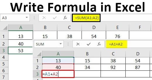
Excel Write Formula (Table of Contents)
- Writing Formula in Excel
- How to Write Formula in Excel?
Writing Formula in Excel
What would be your answer when I ask you, “What is Excel?” A tool that helps to store, slicing and dicing the data plus a tool that can help us calculate sums, percentages, interest rates, etc., right? The most essential as well as an important part of Excel is a formula. The formula is nothing but an equation that allows you to perform various calculations under Microsoft Excel. These formulae are the easiest way of calculation based on the given data. However, being new to Excel, you might not always be able to handle the Excel formulae. It is very easy and simple, though, to add formulae under Excel. This article will try to make you literate about how to write different formulae under Excel, and you will be master in applying the same after going through this article.
Let’s see how we can create/write a formula under Excel.
The first thing we should know is, every Excel formula starts with the equals to sign (‘=’) inside an Excel cell. After this sign, you can write the equation in which you want Excel to perform calculations or any inbuilt function name (Ex. SUM), which performs a calculation and returns the output in a given cell.
How to Write Formula in Excel?
Let’s understand How to Write the formula in excel with a few examples.
You can download this Write Formula Excel Template here – Write Formula Excel Template
Example #1
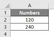
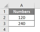
Step 1: Suppose we have two numbers, 120 and 240, in cell A1 and A2, respectively, in the Excel sheet. See the screenshot below:
Now, I want to add these two numbers; We’ll see how this can be achieved.
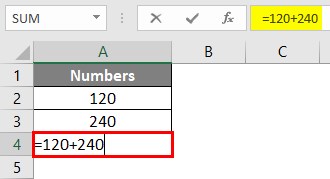
Step 2: In cell A4, start typing the equation by simply using equals to sign and then use 120 + 240 to add these two values up. See the screenshot below for a better understanding.
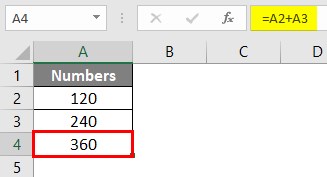
Step 3: Press Enter Key to see the result. You can see 360 as a result of cell A4, as shown below.
This is how a basic formula can be entered under Microsoft Excel. Now, what if we change the numbers in cell A1 and A2 to some different values? Will the formula under cell A3 change values? Well, let’s see by doing so.
Step 4: Change the numbers in cell A1 and A2 to 120 and 240, respectively.
If you will check cell A3, it is still showing the result for old values (i.e. 120 + 140 = 360). Because in cell A3, we have used the equation as 120 + 140. These are values that are fixed and not dynamic ones. Therefore, in order to get rid of such a situation, Excel also provides an option to be able to use dynamic ranges under an equation/formula for that sake.
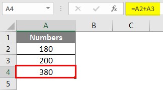
Step 5: In cell A3, tweak the formula to =A2+ A3. What we tried doing here is, instead of giving a number as an argument, we have supplied the cells which contain a number as an argument. This will be beneficial when you change the numbers in cells A2, A3; values in cell A4 will automatically change after performing the operations. This is how making you formula dynamic using a range of cells work.
After using the above formula, the output is shown below:
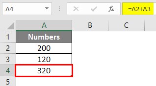
Now, if I change the values under cell A1 and A2, the results in cell A3 will automatically change. See the screenshot below.
Example #2
Excel has a more user-friendly approach when it comes to applying the formula. You just can simply copy-paste the formula from one cell to another by dragging it through. Let’s see how to do it.
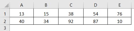
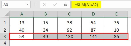
Suppose we have data as shown below across the first and second row of different columns (A to E), and we wanted to get a sum for each column in their third row, respectively. We’ll see how excel works in this situation.
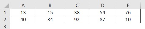
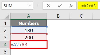
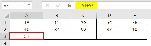
Step 1: In cell A3, create an equation using a dynamic range of cells that sums the values under A1 and A2. You can use =A1+A2 as a formula under cell A3 to get the sum of the numbers within those cells.
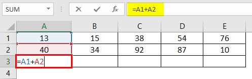
Also, Press Enter key to see the output in cell A3.
Step 2: Now, select the cell A3 and then drag the formula across A3 to E3 to apply the same formula that sums up the first and second row for each column. You should get the output as shown in the screenshot below:
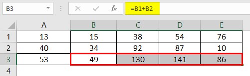
Well, you have multiple ways to achieve this result. You can select the entire third row across column A to E and just press Ctrl + R to copy and paste the formula under cell A3 to other columns. Or else, you can copy the formula under cell A3 by Ctrl + C and paste it one by one in each of B3, C3, D3, E3 to achieve the same result.
Example #3
In this example, we will work on using the built-in Excel functions. How to use the built-in Excel function to perform a task (ex. Summing number across the rows).
Consider the same data as shown in example 2, and we wanted to have sum of the first two rows of each column within the third row. However, this time we will use a built-in Excel function named SUM to achieve this result.
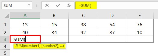
Step 1: In cell A3, start typing =SUM; it will pop up a list of all functions that contain SUM as a keyword. Select the SUM function through that list by double-clicking on it.
Step 2: Select the range of cells A1 to A2 with the use of your computer mouse or laptop touchpad as an argument to the SUM function. Because these are the cells that we wanted to sum up.
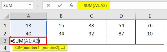
Well, you also can use the comma to separate the values instead of these ranges.
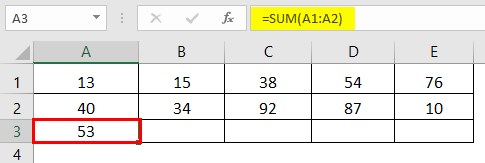
Step 3: Complete this formula by adding closing parentheses at the end of this function and press the Enter key to get the sum of cell A1 and A2 under cell A3.
This function precedes the equation we use in Example 2 by a huge margin when we have tons of data. Ex. Consider you have 5 Lacs Excel Rows, and you wanted to sum those up. You surely would not like to input each cell reference for 5 Lacs of time, would you?
Step 4: You can drag this formula across the different columns for the same row or user Ctrl + R to populate it across all the rows or copy and paste one by one to each column. The choice is all yours. You’ll get the final output as shown below:
This is it from this article. Let’s wrap the things up with some points to be remembered:
Things to Remember About Write Formula in Excel
- In order to be able to use a formula in Excel, you need to start it with equals to sign. You also can start a formula with a Plus or minus sign.
- You can have different operational formulae of your own for subtraction, multiplication, division, squaring a number, etc. However, all these operations are better to do with built-in Excel functions because these functions precede over operational formulae.
Recommended Articles
This is a guide to Write Formula in Excel. Here we discuss How to use Write Formula in Excel along with practical examples and a downloadable excel template. You can also go through our other suggested articles –
- Excel DEGREES Function
- Compare Two Lists in Excel
- Excel Text with Formula
- TIME in Excel