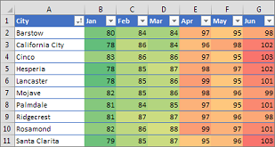
What is a conditional format in excel - Word и Excel - помощь в работе с программами

Conditional formatting can help make patterns and trends in your data more apparent. To use it, you create rules that determine the format of cells based on their values, such as the following monthly temperature data with cell colors tied to cell values.

You can apply conditional formatting to a range of cells (either a selection or a named range), an Excel table, and in Excel for Windows, even a PivotTable report.

Conditional formatting typically works the same way in a range of cells, an Excel table, or a PivotTable report. However, conditional formatting in a PivotTable report has some extra considerations:

There are some conditional formats that don’t work with fields in the Values area of a PivotTable report. For example, you can’t format such fields based on whether they contain unique or duplicate values. These restrictions are mentioned in the remaining sections of this article, where applicable.
If you change the layout of the PivotTable report by filtering, hiding levels, collapsing and expanding levels, or moving a field, the conditional format is maintained as long as the fields in the underlying data are not removed.
The scope of the conditional format for fields in the Values area can be based on the data hierarchy and is determined by all the visible children (the next lower level in a hierarchy) of a parent (the next higher level in a hierarchy) on rows for one or more columns, or columns for one or more rows.

Note: In the data hierarchy, children do not inherit conditional formatting from the parent, and the parent does not inherit conditional formatting from the children.
There are three methods for scoping the conditional format of fields in the Values area: by selection, by corresponding field, and by value field.

The default method of scoping fields in the Values area is by selection. You can change the scoping method to the corresponding field or value field by using the Apply formatting rule to option button, the New Formatting Rule dialog box, or the Edit Formatting Rule dialog box.

Method	Use this method if you want to select
Scoping by selection	A contiguous set of fields in the Values area, such as all of the product totals for one region. A non-contiguous set of fields in the Values area, such as product totals for different regions across levels in the data hierarchy.
Scoping by value field	Avoid making many non-contiguous selections. Conditionally format a set of fields in the Values area for all levels in the hierarchy of data. Include subtotals and grand totals.
Scoping by corresponding field	Avoid making many non-contiguous selections. Conditionally format a set of fields in the Values area for one level in the hierarchy of data. Exclude subtotals. When you conditionally format fields in the Values area for top, bottom, above average, or below average values, the rule is based on all visible values by default. However, when you scope by corresponding field, instead of using all visible values, you can apply the conditional format for each combination of: A column and its parent row field. A row and its parent column field.

Note: Quick Analysis is not available in Excel 2010 and previous versions.

Use the Quick Analysis button to apply selected conditional formatting to the selected data. The Quick Analysis button appears automatically when you select data.

Select the data that you want to conditionally format. The Quick Analysis button appears on the lower-right corner of the selection.
Click the Quick Analysis button , or press Ctrl+Q.
In the pop-up that appears, on the Formatting tab, move your mouse over the different options to see a Live Preview on your data, and then click on the formatting option you want.
Notes:
- The formatting options that appear in the Formatting tab depend on the data you have selected. If your selection contains only text, then the available options are Text, Duplicate, Unique, Equal To, and Clear. When the selection contains only numbers, or both text and numbers, then the options are Data Bars, Colors, Icon Sets, Greater, Top 10%, and Clear.
- Live preview will only render for those formatting options that can be used on your data. For example, if your selected cells don’t contain matching data and you select Duplicate, the live preview will not work.
If the Text that Contains dialog box appears, enter the formatting option you want to apply and click OK.

If you’d like to watch a video that shows how to use Quick Analysis to apply conditional formatting, see Video: Use conditional formatting.

You can download a sample workbook that contains different examples of applying conditional formatting, both with standard rules such as top and bottom, duplicates, Data Bars, Icon Sets and Color Scales, as well as manually creating rules of your own.

Download: Conditional formatting examples in Excel

Color scales are visual guides that help you understand data distribution and variation. A two-color scale helps you compare a range of cells by using a gradation of two colors. The shade of the color represents higher or lower values. For example, in a green and yellow color scale, as shown below, you can specify that higher value cells have a more green color and lower value cells have a more yellow color.

Tip: You can sort cells that have this format by their color — just use the context menu.

Tip: If any cells in the selection contain a formula that returns an error, the conditional formatting is not applied to those cells. To ensure that the conditional formatting is applied to those cells, use an IS or IFERROR function to return a value other than an error value.

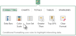
Quick formatting

Select one or more cells in a range, table, or PivotTable report.
On the Home tab, in the Styles group, click the arrow next to Conditional Formatting, and then click Color Scales.
Select a two-color scale.

Hover over the color scale icons to see which icon is a two-color scale. The top color represents higher values, and the bottom color represents lower values.

You can change the method of scoping for fields in the Values area of a PivotTable report by using the Formatting Options button that appears next to a PivotTable field that has conditional formatting applied.

Advanced formatting

Select one or more cells in a range, table, or PivotTable report.
On the Home tab, in the Styles group, click the arrow next to Conditional Formatting, and then click Manage Rules. The Conditional Formatting Rules Manager dialog box appears.
Do one of the following:
- To add a completely new conditional format, click New Rule. The New Formatting Rule dialog box appears.
- To add a new conditional format based on one that is already listed, select the rule, then click Duplicate Rule. The duplicate rule appears in the dialog box. Select the duplicate, then select Edit Rule. The Edit Formatting Rule dialog box appears.
- To change a conditional format, do the following:
  1. Make sure that the appropriate worksheet, table, or PivotTable report is selected in the Show formatting rules for list box.
  2. Optionally, change the range of cells by clicking Collapse Dialog in the Applies to box to temporarily hide the dialog box, by selecting the new range of cells on the worksheet, and then by selecting Expand Dialog.
  3. Select the rule, and then click Edit rule. The Edit Formatting Rule dialog box appears.
Under Apply Rule To, to optionally change the scope for fields in the Values area of a PivotTable report by:
- Selection: Click Selected cells.
- All cells for a Value label: Click All cells showing <Value label> values.
- All cells for a Value label, excluding subtotals and the grand total: Click All cells showing <Value label> values for <Row Label>.
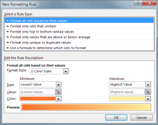
Under Select a Rule Type, click Format all cells based on their values (default).
Under Edit the Rule Description, in the Format Style list box, select 2-Color Scale.
To select a type in the Type box for Minimum and Maximum, do one of the following:
- Format lowest and highest values: Select Lowest Value and Highest Value.
  
  In this case, you do not enter a Minimum and MaximumValue.
- Format a number, date, or time value: Select Number and then enter a Minimum and MaximumValue.
- Format a percentage Percent: Enter a Minimum and MaximumValue.
  
  Valid values are from 0 (zero) to 100. Don’t enter a percent sign.
  
  Use a percentage when you want to visualize all values proportionally because the distribution of values is proportional.
- Format a percentile: Select Percentile and then enter a Minimum and MaximumValue. Valid percentiles are from 0 (zero) to 100.
  
  Use a percentile when you want to visualize a group of high values (such as the top 20thpercentile) in one color grade proportion and low values (such as the bottom 20th percentile) in another color grade proportion, because they represent extreme values that might skew the visualization of your data.
- Format a formula result: Select Formula and then enter values for Minimum and Maximum.
  - The formula must return a number, date, or time value.
  - Start the formula with an equal sign (=).
  - Invalid formulas result in no formatting being applied.
  - It’s a good idea to test the formula to make sure that it doesn’t return an error value.
    Notes:
    - Make sure that the Minimum value is less than the Maximum value.
    - You can choose a different type for the Minimum and Maximum. For example, you can choose a number for Minimum a percentage for Maximum.
To choose a Minimum and Maximum color scale, click Color for each, and then select a color.

If you want to choose additional colors or create a custom color, click More Colors. The color scale you select is shown in the Preview box.

Color scales are visual guides that help you understand data distribution and variation. A three-color scale helps you compare a range of cells by using a gradation of three colors. The shade of the color represents higher, middle, or lower values. For example, in a green, yellow, and red color scale, you can specify that higher value cells have a green color, middle value cells have a yellow color, and lower value cells have a red color.

Tip: You can sort cells that have this format by their color — just use the context menu.

Quick formatting

Select one or more cells in a range, table, or PivotTable report.
On the Home tab, in the Styles group, click the arrow next to Conditional Formatting, and then click Color Scales.
Select a three-color scale. The top color represents higher values, the center color represents middle values, and the bottom color represents lower values.

Hover over the color scale icons to see which icon is a three-color scale.

Advanced formatting

Select one or more cells in a range, table, or PivotTable report.
On the Home tab, in the Styles group, click the arrow next to Conditional Formatting, and then click Manage Rules. The Conditional Formatting Rules Manager dialog box appears.
Do one of the following:
- To add a new conditional format, click New Rule. The New Formatting Rule dialog box appears.
- To add a new conditional format based on one that is already listed, select the rule, then click Duplicate Rule. The duplicate rule is copied and appears in the dialog box. Select the duplicate, then select Edit Rule. The Edit Formatting Rule dialog box appears.
- To change a conditional format, do the following:
  1. Make sure that the appropriate worksheet, table, or PivotTable report is selected in the Show formatting rules for list box.
  2. Optionally, change the range of cells by clicking Collapse Dialog in the Applies to box to temporarily hide the dialog box, by selecting the new range of cells on the worksheet, and then by selecting Expand Dialog.
  3. Select the rule, and then click Edit rule. The Edit Formatting Rule dialog box appears.
Under Apply Rule To, to optionally change the scope for fields in the Values area of a PivotTable report by:
- Selection: Click Just these cells.
- Corresponding field: Click All <value field> cells with the same fields.
- Value field: Click All <value field> cells.
Under Select a Rule Type, click Format all cells based on their values.
Under Edit the Rule Description, in the Format Style list box, select 3-Color Scale.
Select a type for Minimum, Midpoint, and Maximum. Do one of the following:
- Format lowest and highest values: Select a Midpoint.
  
  In this case, you do not enter a Lowest and HighestValue.
- Format a number, date, or time value: Select Number and then enter a value for Minimum, Midpoint, and Maximum.
- Format a percentage: Select Percent and then enter a value for Minimum, Midpoint, and Maximum. Valid values are from 0 (zero) to 100. Do not enter a percent (%) sign.
  
  Use a percentage when you want to visualize all values proportionally, because using a percentage ensures that the distribution of values is proportional.
- Format a percentile: Select Percentile and then enter a value for Minimum, Midpoint, and Maximum.
  
  Valid percentiles are from 0 (zero) to 100.
  
  Use a percentile when you want to visualize a group of high values (such as the top 20th percentile) in one color grade proportion and low values (such as the bottom 20th percentile) in another color grade proportion, because they represent extreme values that might skew the visualization of your data.
- Format a formula result: Select Formula and then enter a value for Minimum, Midpoint, and Maximum.
  
  The formula must return a number, date, or time value. Start the formula with an equal sign (=). Invalid formulas result in no formatting being applied. It’s a good idea to test the formula to make sure that it doesn’t return an error value.
  Notes:
  - You can set minimum, midpoint, and maximum values for the range of cells. Make sure that the value in Minimum is less than the value in Midpoint, which in turn is less than the value in Maximum.
  - You can choose a different type for Minimum, Midpoint, and Maximum. For example, you can choose a Minimum number, Midpoint percentile, and Maximum percent.
  - In many cases, the default Midpoint value of 50 percent works best, but you can adjust this to fit unique requirements.
To choose a Minimum, Midpoint, and Maximum color scale, click Color for each, and then select a color.
- To choose additional colors or create a custom color, click More Colors.
- The color scale you select is shown in the Preview box.

A data bar helps you see the value of a cell relative to other cells. The length of the data bar represents the value in the cell. A longer bar represents a higher value, and a shorter bar represents a lower value. Data bars are useful in spotting higher and lower numbers, especially with large amounts of data, such as top selling and bottom selling toys in a holiday sales report.

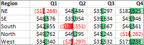
The example shown here uses data bars to highlight dramatic positive and negative values. You can format data bars so that the data bar starts in the middle of the cell, and stretches to the left for negative values.

Tip: If any cells in the range contain a formula that returns an error, the conditional formatting is not applied to those cells. To ensure that the conditional formatting is applied to those cells, use an IS or IFERROR function to return a value (such as 0 or «N/A») instead of an error value.

Quick formatting

Select one or more cells in a range, table, or PivotTable report.
On the Home tab, in the Style group, click the arrow next to Conditional Formatting, click Data Bars, and then select a data bar icon.

You can change the method of scoping for fields in the Values area of a PivotTable report by using the Apply formatting rule to option button.

Advanced formatting

Select one or more cells in a range, table, or PivotTable report.
On the Home tab, in the Styles group, click the arrow next to Conditional Formatting, and then click Manage Rules. The Conditional Formatting Rules Manager dialog box appears.
Do one of the following:
- To add a conditional format, click New Rule. The New Formatting Rule dialog box appears.
- To add a new conditional format based on one that is already listed, select the rule, then click Duplicate Rule. The duplicate rule is copied and appears in the dialog box. Select the duplicate, then select Edit Rule. The Edit Formatting Rule dialog box appears.
- To change a conditional format, do the following:
- 1. Make sure that the appropriate worksheet, table, or PivotTable report is selected in the Show formatting rules for list box.
  2. Optionally, change the range of cells by clicking Collapse Dialog in the Applies to box to temporarily hide the dialog box, by selecting the new range of cells on the worksheet, and then by selecting Expand Dialog.
  3. Select the rule, and then click Edit rule. The Edit Formatting Rule dialog box appears.
Under Apply Rule To, to optionally change the scope for fields in the Values area of a PivotTable report by:
- Selection: Click Just these cells.
- Corresponding field: Click All <value field> cells with the same fields.
- Value field: Click All <value field> cells.
Under Select a Rule Type, click Format all cells based on their values.
Under Edit the Rule Description, in the Format Style list box, select Data Bar.
Select a Minimum and MaximumType. Do one of the following:
- Format lowest and highest values: Select Lowest Value and Highest Value.
  
  In this case, you do not enter a value for Minimum and Maximum.
- Format a number, date, or time value: Select Number and then enter a Minimum and MaximumValue.
- Format a percentage: Select Percent and then enter a value for Minimum and Maximum.
  
  Valid values are from 0 (zero) to 100. Do not enter a percent (%) sign.
  
  Use a percentage when you want to visualize all values proportionally, because using a percentage ensures that the distribution of values is proportional.
- Format a percentile Select Percentile and then enter a value for Minimum and Maximum.
  
  Valid percentiles are from 0 (zero) to 100.
  
  Use a percentile when you want to visualize a group of high values (such as the top 20th percentile) in one data bar proportion and low values (such as the bottom 20th percentile) in another data bar proportion, because they represent extreme values that might skew the visualization of your data.
- Format a formula result Select Formula, and then enter a value for Minimum and Maximum.
  - The formula has to return a number, date, or time value.
  - Start the formula with an equal sign (=).
  - Invalid formulas result in no formatting being applied.
  - It’s a good idea to test the formula to make sure that it doesn’t return an error value.
Notes:
- Make sure that the Minimum value is less than the Maximum value.
- You can choose a different type for Minimum and Maximum. For example, you can choose a Minimum number and a Maximum percent.
To choose a Minimum and Maximum color scale, click Bar Color.

If you want to choose additional colors or create a custom color, click More Colors. The bar color you select is shown in the Preview box.
To show only the data bar and not the value in the cell, select Show Bar Only.
To apply a solid border to data bars, select Solid Border in the Border list box and choose a color for the border.
To choose between a solid bar and a gradiated bar, choose Solid Fill or Gradient Fill in the Fill list box.
To format negative bars, click Negative Value and Axis and then, in the Negative Value and Axis Settings dialog box, choose options for the negative bar fill and border colors. You can choose position settings and a color for the axis. When you are finished selecting options, click OK.
You can change the direction of bars by choosing a setting in the Bar Direction list box. This is set to Context by default, but you can choose between a left-to-right and a right-to-left direction, depending on how you want to present your data.

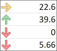
Use an icon set to annotate and classify data into three to five categories separated by a threshold value. Each icon represents a range of values. For example, in the 3 Arrows icon set, the green up arrow represents higher values, the yellow sideways arrow represents middle values, and the red down arrow represents lower values.

Tip: You can sort cells that have this format by their icon — just use the context menu.

The example shown here works with several examples of conditional formatting icon sets.

You can choose to show icons only for cells that meet a condition; for example, displaying a warning icon for those cells that fall below a critical value and no icons for those that exceed it. To do this, you hide icons by selecting No Cell Icon from the icon drop-down list next to the icon when you are setting conditions. You can also create your own combination of icon sets; for example, a green «symbol» check mark, a yellow «traffic light», and a red «flag.»

Quick formatting

Select the cells that you want to conditionally format.
On the Home tab, in the Style group, click the arrow next to Conditional Formatting, click Icon Set, and then select an icon set.

You can change the method of scoping for fields in the Values area of a PivotTable report by using the Apply formatting rule to option button.

Advanced formatting

Select the cells that you want to conditionally format.
On the Home tab, in the Styles group, click the arrow next to Conditional Formatting, and then click Manage Rules. The Conditional Formatting Rules Manager dialog box appears.
Do one of the following:
- To add a conditional format, click New Rule. The New Formatting Rule dialog box appears.
- To add a new conditional format based on one that is already listed, select the rule, then click Duplicate Rule. The duplicate rule is copied and appears in the dialog box. Select the duplicate, then select Edit Rule. The Edit Formatting Rule dialog box appears.
- To change a conditional format, do the following:
  1. Make sure that the appropriate worksheet, table, or PivotTable report is selected in the Show formatting rules for list box.
  2. Optionally, change the range of cells by clicking Collapse Dialog in the Applies to box to temporarily hide the dialog box, by selecting the new range of cells on the worksheet, and then by selecting Expand Dialog.
  3. Select the rule, and then click Edit rule. The Edit Formatting Rule dialog box appears.
Under Apply Rule To, to optionally change the scope for fields in the Values area of a PivotTable report by:
- Selection: Click Just these cells.
- Corresponding field: Click All <value field> cells with the same fields.
- Value field: Click All <value field> cells.
Under Select a Rule Type, click Format all cells based on their values.
Under Edit the Rule Description, in the Format Style list box, select Icon Set.
1. Select an icon set. The default is 3 Traffic Lights (Unrimmed). The number of icons and the default comparison operators and threshold values for each icon can vary for each icon set.
2. You can adjust the comparison operators and threshold values. The default range of values for each icon are equal in size, but you can adjust these to fit your unique requirements. Make sure that the thresholds are in a logical sequence of highest to lowest from top to bottom.
3. Do one of the following:
  - Format a number, date, or time value: Select Number.
  - Format a percentage: Select Percent.
    
    Valid values are from 0 (zero) to 100. Do not enter a percent (%) sign.
    
    Use a percentage when you want to visualize all values proportionally, because using a percentage ensures that the distribution of values is proportional.
  - Format a percentile: Select Percentile. Valid percentiles are from 0 (zero) to 100.
    
    Use a percentile when you want to visualize a group of high values (such as the top 20th percentile) using a particular icon and low values (such as the bottom 20th percentile) using another icon, because they represent extreme values that might skew the visualization of your data.
  - Format a formula result: Select Formula, and then enter a formula in each Value box.
    - The formula must return a number, date, or time value.
    - Start the formula with an equal sign (=).
    - Invalid formulas result in no formatting being applied.
    - It’s a good idea to test the formula to make sure that it doesn’t return an error value.
4. To make the first icon represent lower values and the last icon represent higher values, select Reverse Icon Order.
5. To show only the icon and not the value in the cell, select Show Icon Only.
  Notes:
  - You may need to adjust the column width to accommodate the icon.
  - The size of the icon shown depends on the font size that is used in that cell. As the size of the font is increased, the size of the icon increases proportionally.

To more easily find specific cells, you can format them by using a comparison operator. For example, in an inventory worksheet sorted by categories, you could highlight products with fewer than 10 items on hand in yellow. Or, in a retail store summary worksheet, you might identify all stores with profits greater than 10%, sales volumes less than $100,000, and region equal to «SouthEast.»

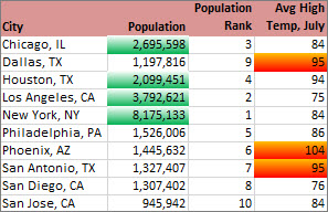
The examples shown here work with examples of built-in conditional formatting criteria, such as Greater Than, and Top %. This formats cities with a population greater than 2,000,000 with a green background and average high temperatures in the top 30% with orange.

Note: You cannot conditionally format fields in the Values area of a PivotTable report by text or by date, only by number.

Quick formatting

Select one or more cells in a range, table, or PivotTable report.
On the Home tab, in the Style group, click the arrow next to Conditional Formatting, and then click Highlight Cells Rules.
Select the command you want, such as Between, Equal To Text that Contains, or A Date Occurring.
Enter the values you want to use, and then select a format.

You can change the method of scoping for fields in the Values area of a PivotTable report by using the Apply formatting rule to option button.

If you’d like to watch videos of these techniques, see Video: Conditionally format text and Video: Conditionally format dates.

Advanced formatting

Select one or more cells in a range, table, or PivotTable report.
On the Home tab, in the Styles group, click the arrow next to Conditional Formatting, and then click Manage Rules. The Conditional Formatting Rules Manager dialog box appears.
Do one of the following:
- To add a conditional format, click New Rule. The New Formatting Rule dialog box appears.
- To add a new conditional format based on one that is already listed, select the rule, then click Duplicate Rule. The duplicate rule is copied and appears in the dialog box. Select the duplicate, then select Edit Rule. The Edit Formatting Rule dialog box appears.
- To change a conditional format, do the following:
- 1. Make sure that the appropriate worksheet, table, or PivotTable report is selected in the Show formatting rules for list box.
  2. Optionally, change the range of cells by clicking Collapse Dialog in the Applies to box to temporarily hide the dialog box, by selecting the new range of cells on the worksheet or on other worksheets, and then by selecting Expand Dialog.
  3. Select the rule, and then click Edit rule. The Edit Formatting Rule dialog box appears.
Under Apply Rule To, to optionally change the scope for fields in the Values area of a PivotTable report by:
- Selection: Click Just these cells.
- Corresponding field: Click All <value field> cells with the same fields.
- Value field: Click All <value field> cells.
Under Select a Rule Type, click Format only cells that contain.
Under Edit the Rule Description, in the Format only cells with list box, do one of the following:
- Format by number, date, or time: Select Cell Value, select a comparison operator, and then enter a number, date, or time.
  
  For example, select Between and then enter 100 and 200, or select Equal to and then enter 1/1/2009.
  
  You can also enter a formula that returns a number, date, or time value.
  - If you enter a formula, start it with an equal sign (=).
  - Invalid formulas result in no formatting being applied.
  - It’s a good idea to test the formula to make sure that it doesn’t return an error value.
- Format by text: Select Specific Text, choosing a comparison operator, and then enter text.
  
  For example, select Contains and then enter Silver, or select Starting with and then enter Tri.
  
  Quotes are included in the search string, and you may use wildcard characters. The maximum length of a string is 255 characters.
  
  You can also enter a formula that returns text.
  - If you enter a formula, start it with an equal sign (=).
  - Invalid formulas result in no formatting being applied.
  - It’s a good idea to test the formula to make sure that it doesn’t return an error value.
  To see a video of this technique, see Video: Conditionally format text.
- Format by date: Select Dates Occurring and then select a date comparison.
  
  For example, select Yesterday or Next week.
  
  To see a video of this technique, see Video: Conditionally format dates.
- Format cells with blanks or no blanks: Select Blanks or No Blanks.
  
  A blank value is a cell that contains no data and is different from a cell that contains one or more spaces (spaces are considered as text).
- Format cells with error or no error values: Select Errors or No Errors.
  
  Error values include: #####, #VALUE!, #DIV/0!, #NAME?, #N/A, #REF!, #NUM!, and #NULL!.
To specify a format, click Format. The Format Cells dialog box appears.
Select the number, font, border, or fill format you want to apply when the cell value meets the condition, and then click OK.

You can choose more than one format. The formats you select are shown in the Preview box.

You can find the highest and lowest values in a range of cells that are based on a cutoff value you specify. For example, you can find the top 5 selling products in a regional report, the bottom 15% products in a customer survey, or the top 25 salaries in a department .

Quick formatting

Select one or more cells in a range, table, or PivotTable report.
On the Home tab, in the Style group, click the arrow next to Conditional Formatting, and then click Top/Bottom Rules.
Select the command you want, such as Top 10 items or Bottom 10 %.
Enter the values you want to use, and then select a format.

You can change the method of scoping for fields in the Values area of a PivotTable report by using the Apply formatting rule to option button.

Advanced formatting

Select one or more cells in a range, table, or PivotTable report.
On the Home tab, in the Styles group, click the arrow next to Conditional Formatting, and then click Manage Rules. The Conditional Formatting Rules Manager dialog box appears.
Do one of the following:
- To add a conditional format, click New Rule. The New Formatting Rule dialog box appears.
- To add a new conditional format based on one that is already listed, select the rule, then click Duplicate Rule. The duplicate rule is copied and appears in the dialog box. Select the duplicate, then select Edit Rule. The Edit Formatting Rule dialog box appears.
- To change a conditional format, do the following:
- 1. Make sure that the appropriate worksheet, table, or PivotTable report is selected in the Show formatting rules for list box.
  2. Optionally, change the range of cells by clicking Collapse Dialog in the Applies to box to temporarily hide the dialog box, by selecting the new range of cells on the worksheet, and then by selecting Expand Dialog.
  3. Select the rule, and then click Edit rule. The Edit Formatting Rule dialog box appears.
Under Apply Rule To, to optionally change the scope fields in the Values area of a PivotTable report by:
- Selection: Click Just these cells.
- Corresponding field: Click All <value field> cells with the same fields.
- Value field: Click All <value field> cells.
Under Select a Rule Type, click Format only top or bottom ranked values.
Under Edit the Rule Description, in the Format values that rank in the list box, select Top or Bottom.
Do one of the following:
- To specify a top or bottom number, enter a number and then clear the % of the selected range box. Valid values are 1 to 1000.
- To specify a top or bottom percentage, enter a number and then select the % of the selected range box. Valid values are 1 to 100.
Optionally, change how the format is applied for fields in the Values area of a PivotTable report that are scoped by corresponding field.

By default, the conditional format is based on all visible values. However when you scope by corresponding field, instead of using all visible values, you can apply the conditional format for each combination of:
- A column and its parent row field, by selecting each Column group.
- A row and its parent column field, by selecting each Row group.
To specify a format, click Format. The Format Cells dialog box appears.
Select the number, font, border, or fill format you want to apply when the cell value meets the condition, and then click OK.

You can choose more than one format. The formats you select are shown in the Preview box.

You can find values above or below an average or standard deviation in a range of cells. For example, you can find the above average performers in an annual performance review or you can locate manufactured materials that fall below two standard deviations in a quality rating.

Quick formatting

Select one or more cells in a range, table, or PivotTable report.
On the Home tab, in the Style group, click the arrow next to Conditional Formatting, and then click Top/Bottom Rules.
Select the command you want, such as Above Average or Below Average.
Enter the values you want to use, and then select a format.

You can change the method of scoping for fields in the Values area of a PivotTable report by using the Apply formatting rule to option button.

Advanced formatting

Select one or more cells in a range, table, or PivotTable report.
On the Home tab, in the Styles group, click the arrow next to Conditional Formatting, and then click Manage Rules. The Conditional Formatting Rules Manager dialog box appears.
Do one of the following:
- To add a conditional format, click New Rule. The New Formatting Rule dialog box appears.
- To add a new conditional format based on one that is already listed, select the rule, then click Duplicate Rule. The duplicate rule is copied and appears in the dialog box. Select the duplicate, then select Edit Rule. The Edit Formatting Rule dialog box appears.
- To change a conditional format, do the following:
- 1. Make sure that the appropriate worksheet, table, or PivotTable report is selected in the Show formatting rules for list box.
  2. Optionally, change the range of cells by clicking Collapse Dialog in the Applies to box to temporarily hide the dialog box, by selecting the new range of cells on the worksheet, and then by selecting Expand Dialog.
  3. Select the rule, and then click Edit rule. The Edit Formatting Rule dialog box appears.
Under Apply Rule To, to optionally change the scope for fields in the Values area of a PivotTable report by:
- Selection: Click Just these cells.
- Corresponding field: Click All <value field> cells with the same fields.
- Value field: Click All <value field> cells.
Under Select a Rule Type, click Format only values that are above or below average.
Under Edit the Rule Description, in the Format values that are list box, do one of the following:
- To format cells that are above or below the average for all of the cells in the range, select Above or Below.
- To format cells that are above or below one, two, or three standard deviations for all of the cells in the range, select a standard deviation.
Optionally, change how the format is applied for fields in the Values area of a PivotTable report that are scoped by corresponding field.

By default, the conditionally format is based on all visible values. However when you scope by corresponding field, instead of using all visible values, you can apply the conditional format for each combination of:
- A column and its parent row field, by selecting each Column group.
- A row and its parent column field, by selecting each Row group.
Click Format to display the Format Cells dialog box.
Select the number, font, border, or fill format you want to apply when the cell value meets the condition, and then click OK.

You can choose more than one format. The formats you select are displayed in the Preview box.

Note: You can’t conditionally format fields in the Values area of a PivotTable report by unique or duplicate values.

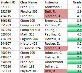
In the example shown here, conditional formatting is used on the Instructor column to find instructors that are teaching more than one class (duplicate instructor names are highlighted in a pale red color). Grade values that are found just once in the Grade column (unique values) are highlighted in a green color.

Quick formatting

Select the cells that you want to conditionally format.
On the Home tab, in the Style group, click the arrow next to Conditional Formatting, and then click Highlight Cells Rules.
Select Duplicate Values.
Enter the values you want to use, and then select a format.

Advanced formatting

Select the cells that you want to conditionally format.
On the Home tab, in the Styles group, click the arrow next to Conditional Formatting, and then click Manage Rules. The Conditional Formatting Rules Manager dialog box appears.
Do one of the following:
- To add a conditional format, click New Rule. The New Formatting Rule dialog box appears.
- To add a new conditional format based on one that is already listed, select the rule, then click Duplicate Rule. The duplicate rule is copied and appears in the dialog box. Select the duplicate, then select Edit Rule. The Edit Formatting Rule dialog box appears.
- To change a conditional format, do the following:
- 1. Make sure that the appropriate worksheet or table is selected in the Show formatting rules for list box.
  2. Optionally, change the range of cells by clicking Collapse Dialog in the Applies to box to temporarily hide the dialog box, by selecting the new range of cells on the worksheet, and then by selecting Expand Dialog.
  3. Select the rule, and then click Edit rule. The Edit Formatting Rule dialog box appears.
Under Select a Rule Type, click Format only unique or duplicate values.
Under Edit the Rule Description, in the Format all list box, select unique or duplicate.
Click Format to display the Format Cells dialog box.
Select the number, font, border, or fill format you want to apply when the cell value meets the condition, and then click OK.

You can choose more than one format. The formats you select are shown in the Preview box.

If none of the above options is what you’re looking for, you can create your own conditional formatting rule in a few simple steps.

Notes: If there’s already a rule defined that you just want to work a bit differently, duplicate the rule and edit it.

Select Home > Conditional Formatting > Manage Rules, then in the Conditional Formatting Rule Manager dialog, select a listed rule and then select Duplicate Rule. The duplicate rule then appears in the list.
Select the duplicate rule, then select Edit Rule.

Select the cells that you want to format.
On the Home tab, click Conditional Formatting > New Rule.
Create your rule and specify its format options, then click OK.

If you don’t see the options that you want, you can use a formula to determine which cells to format — see the next section for steps).

If you don’t see the exact options you need when you create your own conditional formatting rule, you can use a logical formula to specify the formatting criteria. For example, you may want to compare values in a selection to a result returned by a function or evaluate data in cells outside the selected range, which can be in another worksheet in the same workbook. Your formula must return True or False (1 or 0), but you can use conditional logic to string together a set of corresponding conditional formats, such as different colors for each of a small set of text values (for example, product category names).

Note: You can enter cell references in a formula by selecting cells directly on a worksheet or other worksheets. Selecting cells on the worksheet inserts absolute cell references. If you want Excel to adjust the references for each cell in the selected range, use relative cell references. For more information, see Create or change a cell reference and Switch between relative, absolute, and mixed references.

Tip: If any cells contain a formula that returns an error, conditional formatting is not applied to those cells. To address this, use IS functions or an IFERROR function in your formula to return a value that you specify (such as 0, or «N/A») instead of an error value.

On the Home tab, in the Styles group, click the arrow next to Conditional Formatting, and then click Manage Rules.

The Conditional Formatting Rules Manager dialog box appears.
Do one of the following:
- To add a conditional format, click New Rule. The New Formatting Rule dialog box appears.
- To add a new conditional format based on one that is already listed, select the rule, then click Duplicate Rule. The duplicate rule is copied and appears in the dialog box. Select the duplicate, then select Edit Rule. The Edit Formatting Rule dialog box appears.
- To change a conditional format, do the following:
- 1. Make sure that the appropriate worksheet, table, or PivotTable report is selected in the Show formatting rules for list box.
  2. Optionally, change the range of cells by clicking Collapse Dialog in the Applies to box to temporarily hide the dialog box, by selecting the new range of cells on the worksheet or other worksheets, and then by clicking Expand Dialog.
  3. Select the rule, and then click Edit rule. The Edit Formatting Rule dialog box appears.
Under Apply Rule To, to optionally change the scope for fields in the Values area of a PivotTable report, do the following:
- To scope by selection: Click Selected cells.
- To scope by corresponding field: Click All cells showing <Values field> values.
- To scope by Value field: Click All cells showing <Values field> for <Row>.

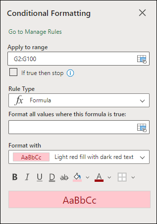
Under Select a Rule Type, click Use a formula to determine which cells to format.

Under Edit the Rule Description, in the Format values where this formula is true list box, enter a formula.

You have to start the formula with an equal sign (=), and the formula must return a logical value of TRUE (1) or FALSE (0).
Click Format to display the Format Cells dialog box.

Select the number, font, border, or fill format you want to apply when the cell value meets the condition, and then click OK.

You can choose more than one format. The formats you select are shown in the Preview box.

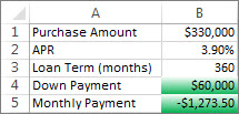
Example 1: Use two conditional formats with criteria that uses AND and OR tests

The following example shows the use of two conditional formatting rules. If the first rule doesn’t apply, the second rule applies.

First rule: a home buyer has budgeted up to $75,000 as a down payment and $1,500 per month as a mortgage payment. If both the down payment and the monthly payments fit these requirements, cells B4 and B5 are formatted green.

Second rule: if either the down payment or the monthly payment doesn’t meet the buyer’s budget, B4 and B5 are formatted red. Change some values, such as the APR, the loan term, the down payment, and the purchase amount to see what happens with the conditionally formatted cells.

Formula for first rule (applies green color)	=AND(IF($B$4<=75000,1),IF(ABS($B$5)<=1500,1))
Formula for second rule (applies red color)	=OR(IF($B$4>=75000,1),IF(ABS($B$5)>=1500,1))

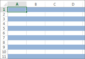
Example 2: Shade every other row by using the MOD and ROW functions

A conditional format applied to every cell in this worksheet shades every other row in the range of cells with a blue cell color. You can select all cells in a worksheet by clicking the square above row 1 and to the left of column A. The MOD function returns a remainder after a number (the first argument) is divided by divisor (the second argument). The ROW function returns the current row number. When you divide the current row number by 2, you always get either a 0 remainder for an even number or a 1 remainder for an odd number. Because 0 is FALSE and 1 is TRUE, every odd numbered row is formatted. The rule uses this formula: =MOD(ROW(),2)=1.

The following video shows you the basics of using formulas with conditional formatting.

If you want to apply an existing formatting style to new or other data on your worksheet, you can use Format Painter to copy the conditional formatting to that data.

Click the cell that has the conditional formatting that you want to copy.
Click Home > Format Painter.

The pointer changes to a paintbrush.

Tip: You can double-click Format Painter if you want to keep using the paintbrush to paste the conditional formatting in other cells.
To paste the conditional formatting, drag the paintbrush across the cells or ranges of cells you want to format.
To stop using the paintbrush, press Esc.

Note: If you’ve used a formula in the rule that applies the conditional formatting, you might have to adjust any cell references in the formula after pasting the conditional format. For more information, see Switch between relative, absolute, and mixed references.

If your worksheet contains conditional formatting, you can quickly locate the cells so that you can copy, change, or delete the conditional formats. Use the Go To Special command to find only cells with a specific conditional format, or to find all cells that have conditional formats.

Find all cells that have a conditional format

Click any cell that does not have a conditional format.
On the Home tab, in the Editing group, click the arrow next to Find & Select, and then click Conditional Formatting.

Find only cells that have the same conditional format

Click any cell that has the conditional format that you want to find.
On the Home tab, in the Editing group, click the arrow next to Find & Select, and then click Go To Special.
Click Conditional formats.
Click Same under Data validation.

When you use conditional formatting, you set up rules that Excel uses to determine when to apply the conditional formatting. To manage these rules, you should understand the order in which these rules are evaluated, what happens when two or more rules conflict, how copying and pasting can affect rule evaluation, how to change the order in which rules are evaluated, and when to stop rule evaluation.

Learn about conditional formatting rule precedence

You create, edit, delete, and view all conditional formatting rules in the workbook by using the Conditional Formatting Rules Manager dialog box. (On the Home tab, click Conditional Formatting, and then click Manage Rules.)

The Conditional Formatting Rules Manager dialog box appears.

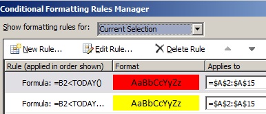
When two or more conditional formatting rules apply, these rules are evaluated in order of precedence (top to bottom) by how they are listed in this dialog box.

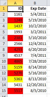
Here’s an example that has expiration dates for ID badges. We want to mark badges that expire within 60 days but are not yet expired with a yellow background color, and expired badges with a red background color.

In this example, cells with employee ID numbers who have certification dates due to expire within 60 days are formatted in yellow, and ID numbers of employees with an expired certification are formatted in red. The rules are shown in the following image.

The first rule (which, if True, sets cell background color to red) tests a date value in column B against the current date (obtained by using the TODAY function in a formula). Assign the formula to the first data value in column B, which is B2. The formula for this rule is =B2<TODAY(). This formula tests the cells in column B (cells B2:B15). If the formula for any cell in column B evaluates to True, its corresponding cell in column A (for example, A5 corresponds to B5, A11 corresponds to B11), is then formatted with a red background color. After all the cells specified under Applies to are evaluated with this first rule, the second rule is tested. This formula checks if values in the B column are less than 60 days from the current date (for example, suppose today’s date is 8/11/2010). The cell in B4, 10/4/2010, is less than 60 days from today, so it evaluates as True, and is formatted with a yellow background color. The formula for this rule is =B2<TODAY()+60. Any cell that was first formatted red by the highest rule in the list is left alone.

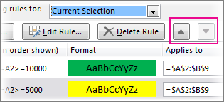
A rule higher in the list has greater precedence than a rule lower in the list. By default, new rules are always added to the top of the list and therefore have a higher precedence, so you’ll want to keep an eye on their order. You can change the order of precedence by using the Move Up and Move Down arrows in the dialog box.
What happens when more than one conditional formatting rule evaluates to True

Sometimes you have more than one conditional formatting rule that evaluates to True. Here’s how rules are applied, first when rules don’t conflict, and then when they do conflict:

When rules don’t conflict For example, if one rule formats a cell with a bold font and another rule formats the same cell with a red color, the cell is formatted with both a bold font and a red color. Because there is no conflict between the two formats, both rules are applied.

When rules conflict For example, one rule sets a cell font color to red and another rule sets a cell font color to green. Because the two rules are in conflict, only one can apply. The rule that is applied is the one that is higher in precedence (higher in the list in the dialog box).
How pasting, filling, and the Format Painter affect conditional formatting rules

While editing your worksheet, you may copy and paste cell values that have conditional formats, fill a range of cells with conditional formats, or use the Format Painter. These operations can affect conditional formatting rule precedence in the following way: a new conditional formatting rule based on the source cells is created for the destination cells.

If you copy and paste cell values that have conditional formats to a worksheet opened in another instance of Excel (another Excel.exe process running at the same time on the computer), no conditional formatting rule is created in the other instance and the format is not copied to that instance.
What happens when a conditional format and a manual format conflict

If a conditional formatting rule evaluates as True, it takes precedence over any existing manual format for the same selection. This means that if they conflict, the conditional formatting applies and the manual format does not. If you delete the conditional formatting rule, the manual formatting for the range of cells remains.

Manual formatting is not listed in the Conditional Formatting Rules Manager dialog box nor is it used to determine precedence.

Controlling when rule evaluation stops by using the Stop If True check box

For backwards compatibility with versions of Excel earlier than Excel 2007, you can select the Stop If True check box in the Manage Rules dialog box to simulate how conditional formatting might appear in those earlier versions of Excel that do not support more than three conditional formatting rules or multiple rules applied to the same range.

For example, if you have more than three conditional formatting rules for a range of cells, and are working with a version of Excel earlier than Excel 2007, that version of Excel:

Evaluates only the first three rules.
Applies the first rule in precedence that is True.
Ignores rules lower in precedence if they are True.

The following table summarizes each possible condition for the first three rules:

If rule	Is	And if rule	Is	And if rule	Is	Then
One	True	Two	True or False	Three	True or False	Rule one is applied and rules two and three are ignored.
One	False	Two	True	Three	True or False	Rule two is applied and rule three is ignored.
One	False	Two	False	Three	True	Rule three is applied.
One	False	Two	False	Three	False	No rules are applied.

You can select or clear the Stop If True check box to change the default behavior:

To evaluate only the first rule, select the Stop If True check box for the first rule.
To evaluate only the first and second rules, select the Stop If True check box for the second rule.

You can’t select or clear the Stop If True check box if the rule formats by using a data bar, color scale, or icon set.

If you’d like to watch a video showing how to manage conditional formatting rules, see Video: Manage conditional formatting.

The order in which conditional formatting rules are evaluated — their precedence — also reflects their relative importance: the higher a rule is on the list of conditional formatting rules, the more important it is. This means that in cases where two conditional formatting rules conflict with each other, the rule that is higher on the list is applied and the rule that is lower on the list is not applied.

On the Home tab, in the Styles group, click the arrow next to Conditional Formatting, and then click Manage Rules.

The Conditional Formatting Rules Manager dialog box appears.

The conditional formatting rules for the current selection are displayed, including the rule type, the format, the range of cells the rule applies to, and the Stop If True setting.

If you don’t see the rule that you want, in the Show formatting rules for list box, make sure that the right range of cells, worksheet, table, or PivotTable report is selected.
Select a rule. Only one rule can be selected at a time.
To move the selected rule up in precedence, click Move Up. To move the selected rule down in precedence, click Move Down.
Optionally, to stop rule evaluation at a specific rule, select the Stop If True check box.

Clear conditional formatting on a worksheet

On the Home tab, click Conditional Formatting > Clear Rules > Clear Rules from Entire Sheet.

Follow these steps if you have conditional formatting in a worksheet, and you need to remove it.

For an entire
worksheet

On the Home tab, click Conditional Formatting > Clear Rules > Clear Rules from Entire Sheet.

In a range of cells

Select the cells that contain the conditional formatting.
Click the Quick Analysis Lens button that appears to the bottom right of the selected data.
Notes:
Quick Analysis Lens will not be visible if:
- All of the cells in the selected range are empty, or
- There is an entry only in the upper-left cell of the selected range, with all of the other cells in the range being empty.
Click Clear Format.

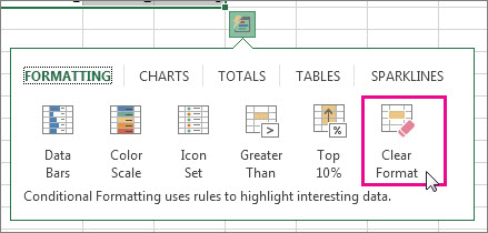
Find and remove the same conditional formats throughout a worksheet

Click on a cell that has the conditional format that you want to remove throughout the worksheet.
On the Home tab, click the arrow next to Find & Select, and then click Go To Special.
Click Conditional formats.
Click Same under Data validation. to select all of the cells that contain the same conditional formatting rules.
On the Home tab, click Conditional Formatting > Clear Rules > Clear Rules from Selected Cells.

Tip: The following sections use examples so you can follow along in Excel for the web. To start, download the Conditional Formatting Examples workbook and save it to OneDrive. Then, open OneDrive in a web browser and select the downloaded file.

Select the cells you want to format, then select Home > Styles > Conditional Formatting > New Rule. You can also open the Conditional Formatting pane and create a new rule without first selecting a range of cells.
Verify or adjust the cells in Apply to range.
Choose a Rule Type and adjust the options to meet your needs.
When finished, select Done and the rule will be applied to your range.

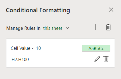
Select a cell which has a conditional format you want to change. Or you can select Home > Styles > Conditional Formatting > Manage Rules to open the Conditional Formatting task pane and select an existing rule.
The Conditional Formatting task pane displays any rules which apply to specific cells or ranges of cells.
Hover over the rule and select Edit by clicking the pencil icon. This opens the task pane for rule editing.
Modify the rule settings and click Done to apply the changes.

The Conditional Formatting task pane provides everything you need for creating, editing, and deleting rules. Use Manage Rules to open the task pane and work with all the Conditional Formatting rules in a selection or a sheet.

In an open workbook, select Home > Styles > Conditional Formatting > Manage Rules.
The Conditional Formatting task pane opens and displays the rules, scoped to your current selection.

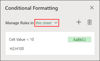
From here, you can:

Choose a different scope on the Manage Rules in menu — for example, choosing this sheet tells Excel to look for all rules on the current sheet.
Add a rule by selecting New Rule (the plus sign).
Delete all rules in scope by selecting Delete All Rules (the garbage can).

You can use a formula to determine how Excel evaluates and formats a cell. Open the Conditional Formatting pane and select an existing rule or create a new rule.

In the Rule Type dropdown, select Formula.

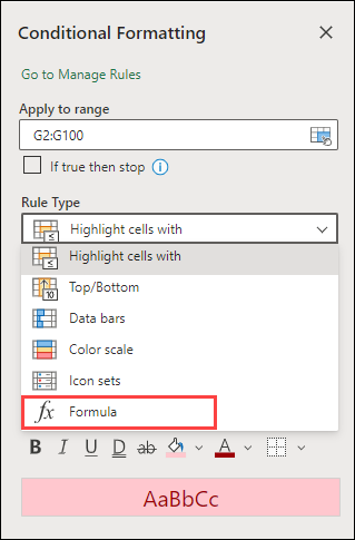
Enter the formula in the box. You can use any formula that returns a logical value of TRUE (1) or FALSE (0), but you can use AND and OR to combine a set of logical checks.

For example, =AND(B3=»Grain»,D3<500) is true for a cell in row 3 if both B3=»Grain» and D3<500 are true.

You can clear conditional formatting in selected cells or the entire worksheet.

To clear conditional formatting in selected cells, select the cells in the worksheet. Then Select Home > Styles > Conditional Formatting > Clear Rules > Clear Rules from Selected Cells.
To clear conditional formatting in the entire worksheet, select Home > Styles > Conditional Formatting > Clear Rules > Clear Rules from Entire Sheet.
To delete conditional formatting rules, select Home > Styles > Conditional Formatting >Manage Rules and use the delete (garbage can) on a specific rule or the Delete all rules button.

Color scales are visual guides which help you understand data distribution and variation. Excel offers both two-color scales and three-color scales.

A two-color scale helps you compare a range of cells by using a gradation of two colors. The shade of the color represents higher or lower values. For example, in a green and yellow color scale, you can specify that higher value cells be more green and lower value cells have a more yellow.

A three-color scale helps you compare a range of cells by using a gradation of three colors. The shade of the color represents higher, middle, or lower values. For example, in a green, yellow, and red color scale, you can specify that higher value cells have a green color, middle value cells have a yellow color, and lower value cells have a red color.

Tip: You can sort cells that have one of these formats by their color — just use the context menu.

Select the cells that you want to conditionally format using color scales.
Click Home > Styles > Conditional Formatting > Color Scales and select a color scale.

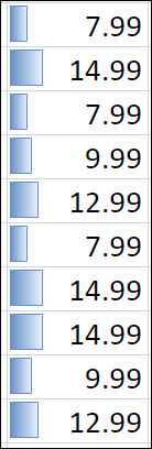
A data bar helps you see the value of a cell relative to other cells. The length of the data bar represents the value in the cell. A longer bar represents a higher value, and a shorter bar represents a lower value. Data bars are useful in spotting higher and lower numbers, especially with large amounts of data, such as top selling and bottom selling toys in a holiday sales report.

Select the cells that you want to conditionally format.
Select Home > Styles > Conditional Formatting > Data Bars and select a style.

Use an icon set to annotate and classify data into three to five categories separated by a threshold value. Each icon represents a range of values. For example, in the 3 Arrows icon set, the green up arrow represents higher values, the yellow sideways arrow represents middle values, and the red down arrow represents lower values.

Select the cells that you want to conditionally format.
Select Home > Styles > Conditional Formatting > Icon Sets and choose an icon set.

This option lets you highlight specific cell values within a range of cells based on their specific contents. This can be especially useful when working with data sorted using a different range.

For example, in an inventory worksheet sorted by categories, you could highlight the names of products where you have fewer than 10 items in stock so it’s easy to see which products need restocking without resorting the data.

Select the cells that you want to conditionally format.
Select Home > Styles > Conditional Formatting > Highlight Cell Rules.
Select the comparison, such as Between, Equal To, Text That Contains, or A Date Occurring.

You can highlight the highest and lowest values in a range of cells which are based on a specified cutoff value.

Some examples of this would include highlighting the top five selling products in a regional report, the bottom 15% products in a customer survey, or the top 25 salaries in a department.

Select the cells that you want to conditionally format.
Select Home > Styles > Conditional Formatting > Top/Bottom Rules.
Select the command you want, such as Top 10 items or Bottom 10 %.
Enter the values you want to use, and select a format (fill, text, or border color).

You can highlight values above or below an average or standard deviation in a range of cells.

For example, you can find the above-average performers in an annual performance review, or locate manufactured materials that fall below two standard deviations in a quality rating.

Select the cells that you want to conditionally format.
Select Home> Styles > Conditional Formatting > Top/Bottom Rules.
Select the option you want, such as Above Average or Below Average.
Enter the values you want to use, and select a format (fill, text, or border color).

Select the cells that you want to conditionally format.
Select Home > Styles > Conditional Formatting > Highlight Cell Rules > Duplicate Values.
Enter the values you want to use, and select a format (fill, text, or border color).

If you want to apply an existing formatting style to other cells on your worksheet, use Format Painter to copy the conditional formatting to that data.

Click the cell that has the conditional formatting you want to copy.
Click Home > Format Painter.

The pointer will change to a paintbrush.

Tip: You can double-click Format Painter if you want to keep using the paintbrush to paste the conditional formatting in other cells.
Drag the paintbrush across the cells or range of cells you want formatted.
To stop using the paintbrush, press Esc.

Note: If you’ve used a formula in the rule that applies the conditional formatting, you might have to adjust relative and absolute references in the formula after pasting the conditional format. For more information, see Switch between relative, absolute, and mixed references.

Note: You can’t use conditional formatting on external references to another workbook.

Need more help?

You can always ask an expert in the Excel Tech Community or get support in the Answers community.

What is Conditional Formatting

Conditional Formatting is a feature in Excel that changes the display of cells whose values meet the Conditional Formatting rule’s criterion. Conditional Formatting makes it very easy to make note of important data whether numerical or non-numerical.

This feature uses graphic means such as highlighting, icons, and data bars to visually cast attention on the required group of values. By doing that, Conditional Formatting makes reviewing and visual analysis of data a very quick task without rearranging the data.

How Does Conditional Formatting Work?

Conditional Formatting applies to cells on the worksheet. At its very basic, you need to select the cells and then apply one of the Conditional Formatting rules. You can choose from the preset options or create your own rule (we will tell you how to do both).

The basic concept is that if a cell meets the Conditional Formatting condition, it results in TRUE and will be reformatted. If it results in FALSE, it won’t be reformatted.

The ease of Conditional Formatting is not only due to the visual impact, but also the automatic selection of the target data. Let’s say e.g., you want the sales figures over $1,000 highlighted below:

If this was a manual task, you would select the cells and then use Fill Color to flag the cells. With Conditional Formatting, you do not have to worry about selecting the right cells.

If you select all the data cells from column C, Conditional Formatting will do the job of flagging the right cells according to the set rule. Therefore, select all the cells with the sales figures:

Now where is this Conditional Formatting feature we’ve been talking about? In the Home tab, you will find the Conditional Formatting icon in the Styles group.

Conditional Formatting has highlighted the cells from the dataset that had sales of over $1,000:

Want to see how that’s done? Highlighting is not the only thing this feature does so you won’t get this formatting by just a click on the icon. Conditional Formatting has a bunch of options in its menu:

We’ll talk about creating different types of rules to conditionally format cells ahead in this tutorial.

Notes:

Conditional Formatting deals with numbers, dates, time, and text strings and while some rules won’t work for text, they all work for numbers, dates, and time (excluding the Text that Contains rule).

Conditional Formatting is dynamic. This means that it will adjust its result according to changes within the data. E.g. if a value that was previously not highlighted with Conditional Formatting is changed and meets the criterion of the applied rule, it will then be highlighted.

If you intend to make additional entries to the data and want Conditional Formatting to accommodate them, you can try leaving the references in the formula free if it doesn’t hinder the results of the Conditional Formatting rule(s).

E.g. enter B3 instead of $B$3. Another option is to force Conditional Formatting to include more rows/columns by using the Format Painter parallelly to the new row/column and then adding the data. Otherwise, you can simply extend the range in the Rules Manager.

Any Conditional Formatting action can be undone with Undo or Ctrl + Z including adding a new rule, deleting a rule, applying a rule, and editing a rule.

Cell Formatting You Can/Cannot Change

The format of a cell comprises several elements e.g., font size, font color, color fill, border, row height, etc. and there is only so much that Conditional Formatting can do. Some elements of the cell format can be changed by Conditional Formatting while others can’t. To keep your expectations real, let’s classify the elements of cell formats into what Conditional Formatting can and cannot change.

The Format Cells dialog box is what you will get when you click on the (Custom) Format button while dealing with a formatting rule. We can open Format Cells through Conditional Formatting and see what the feature will allow. Good idea. Let’s go through the Format Cells dialog box tab by tab, beginning with the Number tab:

All Number formats are applicable through Conditional Formatting including Custom Number Format.

The next tab is the Font tab:

In the Font tab, the elements of the font in the cell that we will be able to change with Conditional Formatting are font style (bold, italic, etc.), color, underline, and effects (strikethrough, superscript, etc.).

The rest of the elements that are grayed out are not accessible and cannot be changed using the Conditional Formatting feature. These are font family and size.

Moving on to the Border tab:

Border styles are changeable from the available options. The Border color can also be altered.

If you’re familiar with Borders in Excel, you’ll know that the Border styles in Conditional Formatting are limited. To be more specific, the double border and thicker borders are missing. So, the deduction is that border thickness cannot be changed with Conditional Formatting.

Let’s see what we can do fill-wise in the Fill tab:

All the Fill options can be edited in Conditional Formatting.

All in all, other than some font and border elements, all others can be changed through Conditional Formatting. Comparing this window to the regular Format Cells dialog box, we notice we have a couple of tabs missing; the Alignment and Protection tabs.

Conditional Formatting does not give access to these tabs which implies that the feature cannot change the text alignment or the protection of a cell via the feature.

Note:

Conditional Formatting is only a formatting feature and does not affect the value of a cell.

Conditional Formatting Options

Let’s refer back to the Conditional Formatting menu:

We’re going to tackle each item in this menu so…

Let’s get formatting! Conditionally though…

Highlight Cells Rules

One of the most commonly used features of Conditional Formatting is Highlight Cells. Selected cells will be highlighted according to a chosen cell highlighting rule. There are a few interesting preset rules available in this category e.g., highlighting a particular value, a cell that contains the given text, etc. Let’s go over all the options so you know how to apply them to your Excel work.

Greater Than…

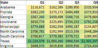
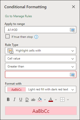
The Greater Than rule highlights numerical values greater than the user-provided value. This option can be used to cast focus on high-performing products, the highest tier in an age group, amounts over a borderline value, etc. If that sounds like what you’re targeting, you can use the steps below to highlight cells with numerical values greater than the supplied value.

As an example, we’re taking some sales data categorized by product and state. For now, we want to find out which product is giving us the highest sales and from which region. Here’s how we do it:

Select the relevant cells with the numeric values from where you want the highlighted cells.

Select the Home tab’s Conditional Formatting icon in the Styles Point to Highlight Cells Rules and select the Greater Than rule.

This rule will lead to a dialog box where you can set the numerical value and format intended for the highlighted cell. Gauging the selected cells, Excel will already provide you with an example value in the dialog box.
In the Greater Than dialog box, adjust the numerical value in the text box. *(Read note below). The numbers that are greater than this number will be highlighted in the dataset. E.g. in our case, we want sales greater than $600 to be highlighted.
You can also choose another format for the highlighted cells from the drop-down list in the dialog box.

When done setting the number and format, click on the OK button of the dialog box.

The dialog box will close and the cells with sales greater than $600 will be highlighted in the chosen format:

Notes:

* The number $600 can also be added as a cell reference by clicking on the applicable cell with the blinking cursor in the text box of the dialog box. This would be the easier way if the value you want to set is a decimal.

By default, the highlight format for the cells will be light red fill with dark red text. This can quickly be changed to another ready format from the drop-down menu in the dialog box which also carries an option of a custom format. You’ll see how to set a custom highlight format in a while.

Less Than…

Let’s squeeze in the opposite of what we did just now in the same example. With the same concept, Conditional Formatting also gives the option of highlighting cells with values less than a provided number.

After applying this formatting rule in our case example, we’ll be able to see the top and flop products together on the same sheet, distinguished by a different format. See the steps and find out what that would look like:

Select the data cells and go to the Conditional Formatting icon in the Home From the menu, head to Highlight Cells Rules and now select the Less Than option.

Now you will have a Less Than dialog box, much like the one we saw earlier.
Enter the number in the text field. Conditional Formatting will use this number to determine which cells should be highlighted. For our case, we are going with $150 so that values under 150 will be flagged.
Change the format if you wish. We are aiming to highlight the bottom values so the default red format is good with us.

Then hit the OK

From the selected cells, the products with sales lower than $150 are highlighted in the default red format:

Since we’ve used the Less Than rule with the Greater Than rule, we get a quick view of the hot and not products. Notice how we’re halfway to making a heat map?

Now that we mention it, Conditional Formatting is already ahead of us and allows us to create heat maps in Excel. How? You’ll see later. Hint: Color Scales.

Between…

The Between option highlights numerical values between 2 given numbers. This can be particularly helpful e.g., color coding an age group of interest. We’ll take a simple example and show you how it works.

In our simple example case, 10 people take part in a 5-question quiz to win a prize. A point is awarded for each question so we’d like to see how many participants scored averagely, say between 2 and 4. This is how to use Conditional Formatting to highlight values between 2 numbers inclusive:

Select the number cells and open the Conditional Formatting menu from the Home Select Highlight Cells Rules > Between.

A dialog box will appear for you to set the range of values and the highlighting format.
Enter the numbers between which you want values highlighted in the dataset.
This range works inclusively and the top and bottom values will also be highlighted.
Choose a format for the highlighted cells and then click on the OK

We have set the values between 2 and 4 to be highlighted with a yellow fill:

Equal To…

But more importantly, wouldn’t you want to find out the winners? Of course you would. That would require highlighting the cells with a score of 5. Conditional Formatting makes highlighting cells carrying a specific value a task done in seconds.

Using the Equal To option in Highlight Cells Rules, we have mentioned the steps to highlight cells of a single value:

Select the cells with the numbers.
Go to Home tab > Conditional Formatting icon > Highlight Cells Rules > Equal To.

In the text box in the Equal To dialog box, enter the number you want highlighted in the dataset and select the format for those highlighted cells.

When you press the OK button, the entered number will be highlighted in the set format:

Text that Contains…

By now it looks like Highlight Cells Rules only likes working with numbers but that’s not the case. Have you ever had difficulty finding a part of text from a text string because it was not categorized appropriately?

We’ve been there too. If the target is to locate those cells or split the text, you can use Ctrl + F and other options to divide the text but if you want the text string found and the cell containing the text highlighted, nothing does it better than Conditional Formatting.

Follow the steps relating to the example ahead to find and highlight cells that contain the provided text with Conditional Formatting:

In this example, we have a list of fragrances with their brand names both mentioned together in column B. If we want to see which perfumes are made by a particular brand, taking e.g. Chanel, we will start by:

Select the cells containing the data that you want to check.
In the Conditional Formatting menu (Home tab > Style group), select Highlight Cells Rules and then the Text that Contains

In the text field add the string of text you want to find in the data cells.
To choose your format for the highlights, click on Custom Format from the drop-down menu.

We’ve set a custom format with an orange color fill.

Click OK on both windows to close them and apply Conditional Formatting to the cells in the custom format.

As per the set format and text value entered in the dialog box, the cells containing that text value will be highlighted:

A Date Occurring…

Another type of number value Conditional Formatting runs with is dates. With the A Date Occurring option, dates that range from the previous month to the next month can be highlighted.

For specific dates, you’ll have to resort to other Conditional Formatting rules since this rule does the job of highlighting dates relative to the current date e.g. dates from last week, yesterday, next month, etc.

Would be easier with an example? We think so too. Our example shows the order dates and scheduled delivery dates of a range of products. Take the current date as 25^th of July. We want to highlight the dates from the list that are scheduled to be delivered the next day i.e. on the 26^th of July.

With the following steps, you can use the A Date Occurring rule to highlight the date cells relative to the date option selected.

Select the cells with the dates.
Our target is to highlight the delivery date cells so we’ll select the date cells from column D.

From the Home tab, select the Conditional Formatting button, Highlight Cells Rules, A Date Occurring.

In the dialog box, open the first drop-down menu and select the required option.
In our example, we want the dates for the next day highlighted and hence, we will go with the ‘Tomorrow’ option.

Use the next drop-down menu to change the highlighted cells format.

The cells with the date 26^th July 2022 in column D will be highlighted according to the selected format:

Note: The plus point of using A Date Occurring instead of forming a rule to highlight the 26^th specifically is that this option will work relatively; with the changing date, the dates for the next day will automatically be highlighted e.g., on the 26^th, 27^th will be highlighted.

Duplicate Values…

When dealing with large data, there is a possibility of doubly-made entries and duplicate values. In most cases, you would want to avoid this and a good place to start would be to highlight them. Let’s see how to highlight repeat values with Conditional Formatting using an example.

In this example, we have used the RANDBETWEEN function to return 10 random numbers from 1 to 20. On its own, RANDBETWEEN doesn’t return unique numbers and there will be duplicates. Let’s check our data for duplicates with Conditional Formatting’s Duplicate Values option.

Select the range you want to be searched for repetitions.
From the Styles group in the Home tab, go to the Conditional Formatting’s Highlight Cells Rules menu and select Duplicate Values.

In the dialog box, the default selection is “Duplicate” *(read note below) so you only need to change the default format if you want to.

Select the OK command to close the dialog box and apply the Conditional Formatting for duplicate values:

* There is also an option to highlight unique values as shown in the example shot.

Top/Bottom Rules

We can now move on to the second item in the Conditional Formatting menu. The Top/Bottom Rules help the user format the top or bottom number values. In this set of rules, we have options for highlighting the top/bottom items, top/bottom x%, and the above/below average items.

Keep in mind that Top/Bottom Rules do not work on non-number values so text values, you’re out for now.

Also, we have a very interesting finding. The top/bottom percentage rule is a quick way to highlight the required percentile! If you’ve worked with percentiles before, you’ll find this particular feature rather handy.

Let’s start exploring the preset options in the Top/Bottom Rules one by one.

Top 10 Items…

Say you have a long list of expenses (don’t we all) and want to point out the top 10 items in the list that are taking up the most bucks. The top 5 priciest products, the top 15 songs from a database with the most hits; this is what you can use the Top 10 Items option for.

Another instance where you can use the Top 10 Items rule is the example ahead. We have the test marks out of 50 in a class of 10 students. Since our data consists of 10 students, we obviously won’t be searching for the top “10”.

Gladly, we can change this number. Let’s aim to find the top 3 scores on this test with Conditional Formatting’s Top 10 Items rule:

Select the cells from the data containing the numbers, dates, or time.

Now open the Conditional Formatting menu and go to Top/Bottom Rules and then Top 10 Items.

The Top 10 Items dialog box has the number 10 suggested by default.
Change the number ‘10’ according to your requirement using the spin button or by editing the value in the text box.
At this point, you can also change the highlight format through the drop-down menu.

To apply the format, close the dialog box with the OK

The top 3 items in the list are highlighted. In our case example, one of the marks has a repeat value i.e. 39 which is why you see 4 highlighted cells below:

The next rule in line is Top 10 % but we’ll bump up Bottom 10 Items because doesn’t that make a better succession to Top 10 Items?

Bottom 10 Items…

The Bottom 10 Items rule highlights, well yes, the bottom items. It works opposite of the Top 10 Items rule. Why would we want to bring the bottom items to notice? This could be for detecting the lowest performance products, months of lowest sales in a report, lowest scores, etc.

Taking the example from the section above, we will now study the 3 lowest scores. Looking at the range of bottom scores will help us ascertain if it’s just the lowest score that’s pulling the percentile down or if more students have scored similarly.

Let’s go ahead with using Conditional Formatting’s Bottom 10 Items rule to highlight the bottom 3 items in our case example:

In the dataset, select the range with the numbers.
From the Top/Bottom Rules in Conditional Formatting, select the Bottom 10 Items

Change the number in the dialog box in line with the number of bottom items you want highlighted.
Set the format of choice for the highlighted cells.

When done, use the OK button to close the dialog box and highlight the relevant cells.

Here you can see that the bottom 3 items are highlighted in the chosen format:

The bottom 3 marks are 31, 33, and 34 showing that the lowest score is not the only reason for the lower percentiles since two other students out of 10 have scored likewise.

Top 10 %…

This is a very interesting rule. The Top 10 % rule works out the percentage from the numbers in the selected cells and highlights the cells with the numbers that fall in the top 10% (percentage can be adjusted).

With Excel putting in so much effort, isn’t life that much easier? Let’s find out if it is so! To highlight the top x% with Conditional Formatting use these steps:

Begin with selecting the data cells with the numbers.
Go to Home tab > Styles group > Conditional Formatting button > Top/Bottom Rules > Top 10 %.

In the text field of the dialog box, you can change the percentage number which by default is set at 10.
We’ll leave it at 10 since we are also aiming to calculate the top 10%. To calculate e.g. the bottom 25%, change this number to 25 in the dialog box.
Use the drop-down menu in the dialog box to change the format of cells that are to be highlighted.

Click on the OK button when done.

The marks falling in the top 10% of the selected cells will be highlighted:

Bottom 10 %…

After the Top 10 % follows the Bottom 10 %. The antithesis of what we just saw earlier, the Bottom 10 % rule takes the numbers in the selected cells to highlight the values that fall in the lower 10% of the numbers.

Carrying forward the previous example, let’s test how this rule works to highlight the bottom 10% with the top 10% already highlighted.

Select the cells from the dataset and go to the Conditional Formatting options to select the Bottom 10 % rule in the Top/Bottom Rules.

Set the format for highlighting and the number for the percentage in the Bottom 10% dialog box.

When the OK command is pressed, the bottom 10% of the values will be highlighted.

Percentage or Percentile?

Let’s analyze what is happening here now that we’ve got the top and bottom 10% highlighted. And for discussion’s sake, we’re only talking about 10% here (though this can be any other percentage). If you think about regular percentage, 10% of 50 marks should be 5 marks so the top 10% (i.e. 90%) should be 45 marks.

In the Top 10 % rule, Conditional Formatting determines the top 10% only from the numbers selected. That means, this rule is unconcerned with the actual percentage because it is taking the lowest and highest values in the selection as 0% and 100%. Does that sound familiar? That is also the concept of percentile.

This finding is in line with percentile computations. If you look at the example shot above, we have calculated the 10th and 90th percentiles as 31.2 and 37.5 with the PERCENTILE.INC function. Compare this to the cells highlighted by Conditional Formatting.

For the top 10%, we have 31 marks highlighted (falls under 31.2 marks) and for the bottom 10%, 48 marks have been highlighted (going over 47.5 marks).

On this deduction, we can conclude that the Top and Bottom 10 % rules work as percentiles and can be a quick visual percentile map! Fascinating!

Above Average…

This section will further confirm the percentile theory. The Above Average rule in the Top/Bottom Rules highlights all the number values in the selection that are above the average of those numbers i.e. above 50% or the median.

Our previous example case has the median calculated using the PERCENTILE.INC function. Therefore, we’ll show you the steps to highlight the cells that are above the average of those numbers using Conditional Formatting’s Above Average rule.

After selecting the cells with the numbers, click on the Conditional Formatting icon to access the Above Average option from the Top/Bottom Rules.

You will be led to the Above Average dialog box:
There is only one setting in this dialog box and i.e. the format of the highlighted cells.
This rule only focuses on the average or 50% since the percentages can be adjusted in the Top and Bottom 10% rules.

Hit OK when done and find one half of the values above average highlighted in the set format:

Below Average…

And for the other half of the average, this rule highlights the values from the cell selection that are below the average of those numbers.

Let’s piece this together with the case example from above and highlight the values below the average with Conditional Formatting’s Below Average rule with the steps mentioned ahead:

Select the data with the numbers from where you want to calculate the average.
Apply the Below Average rule by selecting Home tab, Conditional Formatting icon, Top/Bottom Rules, Below Average

Set the preferred format for the highlighted values in the dialog box and click on the OK

The values below average in the selected cells will be highlighted in the set format:

Calculated as per the PERCENTILE.INC function, 50% of these numbers are above 37.5 marks, and 50% fall below. Evaluating the results of the highlights, we can see that Conditional Formatting tallies with the percentile system.

Data Bars

While numbers are crucial for calculations and analysis, the best type of data is one that is easily perceptible with distinguished high and low points. These two Conditional Formatting features (namely Data Bars and Color Scales) fulfill the convenience of giving the data a visual representation.

First comes Data Bars. Data Bars won’t be a very alien concept if you’ve seen bar charts. It’s like a personal bar for each cell.

Data Bars underlays a single bar in the selected cell. For a selected range, a bar will be added to each cell in line with and under the cell’s number value. The value of the cell determines and is directly proportional to the length of its Data Bar; small number – small bar.

In case you would ever want to add Data Bars to your dataset, we suggest these steps using Conditional Formatting in a simple example:

Select the cells you want to add the Data Bars
In the Home tab, head to the Styles group to access the Conditional Formatting Hover the cursor on Data Bars to reveal the menu. Choose the Data Bar style from the menu from Gradient Fill or Solid Fill. The color can also be chosen or you can create your own style from More Rules.

The Data Bars will be entered in the chosen style:

If you want to go for customized Data Bars, click on More Rules in the Data Bars menu.

In the Type fields, you have various options to change the type of Data Bar e.g., the one we just showed you was simply according to the numerical value. You can change this to percentile, percentage, etc. instead of numerical value.

These are fairly detailed options including changes for the bar direction (left to right, right to left) and Negative Value and Axis settings for when the data includes negative numbers.

Note: Data Bars and Icon Sets will also not affect the cell value as Conditional Formatting is only a formatting feature.

Color Scales

Remember we spoke of heat maps earlier? Now is a good time to come back to that. Excel can speedily ready a heat map for your dataset with Color Scales in Conditional Formatting. Think of it as color coding for the numbers in your data e.g., on a scale of red to green, the smallest number is red and the largest number is green. If you’re the one who had every color highlighter for studies or work, you’ll love this!

The perk of a Color Scale is that it can tell the position of any number in the range by the shade of the cell’s color. We’ll put Color Scales into action now with a very black and white example of product and state-wise categorized sales data.

Select the relevant range for adding the Color Scale.

Select Conditional Formatting from the Ribbon in the Home Hover the mouse pointer on Color Scales to open up some preset options.

Select the favored Color Scale or you can use the More Rules option to form a custom 2 or 3-Color Scale where you can also specify the minimum, mid (if any), and maximum values for the color points.

When the Color Scale is selected, it will be immediately applied to the selected range.

See how that works to give an instantaneous overview of the values? Maybe some of your highlighters have already made their way to the garbage.

Icon Sets

This is another very cool feature called Icon Sets that shows in what range a cell’s value lies according to its icon added by Conditional Formatting. Icon Sets applies a set of icons to the cells in selection. The Icon Sets represent the lowest, highest, and multiple mid (can be excluded) values that are editable.

Let’s apply Icon Sets in an example of quality assurance scores for 10 products. See what to do below to use Icon Sets in Conditional Formatting.

Select the number cells for applying Icon Sets.
Go to the Home tab > Conditional Formatting icon and point to the Icon Sets
If you want to apply Icon Sets with the default settings* click on the relevant Icon Set from the menu. To change the settings according to which the icons will be added, click on the More Rules option in the Icon Sets menu.

You will see a New Formatting Rule dialog box:

Now make the changes as per your preference. These are the changes made for our case example:
Pick the style from the Icon Style drop-down menu.
Change the Type from Percentage to Number so that the Icons are entered according to the number of the cell, not the percentage of the number against all the selected cells.
Set the numbers in the Value fields as the range for each icon. E.g. for values 12 and higher, a green check mark will be returned. Values between 8 and 11 will be assigned a yellow exclamation point and for lower numbers, there will be a red cross mark.

If you want the numbers overwritten, click the Show Icon Only checkbox.
Click on the OK button after the changes are made.

The Icon Set has been entered with the values in the selected cells in accordance with the changed settings:

* When applied, Icon Sets will enter icons to the selected cells in their default settings. The icons are set at equal percentage intervals e.g., a 3-Icon Set is applied at 33 percent intervals, 4-Icon Set at 25 percent intervals and 5-Icon Set at 20 percent intervals.

Tip: If you want the values and icons in separate columns, paste the values in another column, apply the Icon Set and overwrite the values by tick-marking the Show Icon Only checkbox in the settings.

Change Conditional Formatting Rule

To change a rule in Conditional Formatting, you need access to the Conditional Formatting Rules Manager. The Rule Manager enlists all the Conditional Formatting rules and allows changing, deleting, creating, and stacking rules according to preference of application.

You would want to change a rule in the case that an incorrect rule has been formed or some element of the rule needs editing and the original rule is not required anymore e.g., instead of the top 10 items, we want to highlight the top 3 items and don’t need to keep the top 10 items highlighted.

The original rule will not be overwritten if a new rule is formed.

See how to change a Conditional Formatting Rule using the steps written below:

Select the range to which the rule applies.
If you’re unclear about the range, you can select just a single cell or make a rough estimate of the range and the rules applied to the selected cell/range will be shown in the Rules Manager. Otherwise, you can select the entire sheet from the active worksheet or even from the Rules Manager.
To open the Rules Manager, open the Conditional Formatting options from the Home tab and select Manage Rules.

The Conditional Formatting Rules Manager lists the created rules for the cells selected on the worksheet. You can change this in the Show formatting rules for drop-down menu at the top in the Rules Manager.

Select the rule you want to edit and click on the Edit Rule Alternatively, you can double-click a rule to edit it.

Use the Edit Formatting Rule window to change the rule description and/or rule type.

When you press the OK command, the edited rule will show in the Rules Manager.

Press the OK button to apply the edited Conditional Formatting Rule.

As a result of the rule being changed from top 3 to top 2, only the top 2 numbers are highlighted in the example case above.

Delete Conditional Formatting Rule

Conditional Formatting Rules are deleted from the Conditional Formatting Rule Manager.

To completely remove a rule from the worksheet, you will have to delete the rule. It may also be easier to create a new rule instead of editing an old one in which case, you will have to delete the old rule. Deleting a rule is reversible by undoing the action so if you accidentally lose a rule, you can get it back.

Check these steps on how to delete a Conditional Formatting Rule:

Select a cell in the range of the rule that you want to delete.
Go to Home tab > Style group > Conditional Formatting > Manage Rules.

This option opens the Conditional Formatting Rule Manager.
Click on the rule and hit the Delete Rule

The rule will be deleted without any confirmation. It’s not really a problem, if you delete the wrong rule, hit the Cancel command. If you’ve already pressed the OK button, you can hit Undo; the rule will be back.
After deleting the rule, select the OK

The rule will be deleted and the formatting relevant to that rule will be cleared:

Deleting all Rules from Selection

One last thing left in the Conditional Formatting menu. While it’s easy to delete whichever rule from the Rules Manager, it can be tiresome carefully looking at absolutely referred ranges to see which rule applies where especially if you aim to delete the rules only from a specific range without deleting others.

To clear rules from a specific range, select the cells and go to Conditional Formatting icon > Clear Rules > Clear Rules from Selected Cells.

If you want to delete all the rules from the worksheet, you can go for Clear Rules from Entire Sheet instead of deleting the rules one by one from the Rules Manager. The other two options become available if there is an Excel Table or PivotTable present on the worksheet.

New Rule

New rules will not overwrite rules, they will be stacked (newest first unless the order is changed in the Rules Manager if any results are overlapping.

While more favorably you can create a new rule from Conditional Formatting’s New Rule option, a few options are also available in the Quick Analysis tool. The icon appears in the bottom-right corner when you select more than one data cell:

Click on this icon to see the options.

This is the little cousin of Conditional Formatting with 5 rules and an option to clear formatting from the selected area. Conditional Formatting in the Quick Analysis tool will add new rules to the selected range; it won’t overwrite rules.

New Formatting Rule Dialog Box

This dialog box will come into play with 3 actions; creating a new rule, editing a rule, and when you select More Rules in the Conditional Formatting menu. Most of the items in Rule Type are pretty much an extension of the options in the Conditional Formatting menu and some of them you will see in the sections later. Let’s quickly go over the Rule Types and what they contain.

Format all cells based on their values

This rule type has detailed options regarding Color Scales, Data Bars, and Icon Sets.

Format only cells that contain

This one’s intriguing. This rule type has varied options for formatting cells based on a specified value (number and text), date, blanks, no blanks, errors, and error-free cells.

Format only top or bottom ranked values

Here we can select top or bottom items or percentages to format the cells accordingly.

Format only values that are above or below average

This type is for widening the Above and Below Average rule in Conditional Formatting. We can format the cells with the average inclusive or exclusive and can also see some standard deviation options (hello math and stats).

Format only unique or duplicate values

Simply includes duplicate and unique values formatting.

Use a formula to determine which cells to format

If none of the preset rules and rule types suit your Excel action, you can get the needful done by entering a formula here.

Common Use Cases of Conditional Formatting

Now that we’ve covered everything contained in the Conditional Formatting menu, we can move on to scenarios that would commonly use Conditional Formatting. Some have already been discussed above. Let’s see what else Conditional Formatting can do.

Use Conditional Formatting to Highlight Alternate Rows

Highlighting alternate rows is nothing big for Conditional Formatting. And while this can also be done using a preset format in Excel Tables, you might not want to convert your range to a Table.

There are quite a few formulas that can be used with Conditional Formatting to highlight every other row. We’ll go with the one used in our example case below because it’s easy to tweak for your range and requirement. Let’s see the formula and how to apply it using Conditional Formatting to highlight alternate rows:

On the worksheet, select the range where you want the alternately highlighted rows.
Click on the Conditional formatting button in the Home tab and choose New Rule.

There are 3 steps you need to take in the New Formatting Rule dialog box.
In the Select a Rule Type section, choose Use a formula to determine which cells to format.
In the given text box, enter this formula to highlight every other row:

=INT(MOD(ROW(),2))

Explanation below*

Hit the Format button to set the format for the highlighted rows.

One more step, select the OK
That’s alternate rows highlighted for you with Conditional Formatting:

The ROW function will take the number of the row the formula is entered in. Starting from the first row, in our example case, the number will be 3. The MOD function will return the remainder after 3 is divided by the supplied number 2. We are left with the number 1. The INT function is there to round the remainder down to an integer. Left with 1, the formula highlights the first row.

This formula can highlight even rows for you. So you can use this formula instead:

=INT(MOD(ROW()+1,2))

With the added 1, the formula will highlight the rows starting from the second row (the remainder 1 added to the extra 1 in this formula equals 2) in the range:

Use Conditional Formatting to Find & Highlight Blank Cell Rows

There are two aspects to highlighting blank cells in Excel. The first is only highlighting the blank cells. The second is highlighting the entire row or column in the dataset containing the blank cell.

Highlighting blank cells with Conditional Formatting doesn’t require any formula. There’s an in-built setting to highlight blank cells in the New Formatting Rule dialog box.

To enable it, select the area containing the blank cells and go to Conditional Formatting menu > New Rule. In the dialog box, select Format only cells that contain as the rule type and Blanks in the drop-down menu. Set the format.

This setting will highlight blank cells in the selected range. We had selected D6:D15.

To highlight the full row (let’s say from B7 to D7 when D7 is found blank), you’ll have to include a formula in the works so we can control highlighting the full row of the table. Here’s what you need to do to highlight the full row containing the blank cells with Conditional Formatting:

Select the range in the dataset containing the blank cells. You need to select the area that you would want to be highlighted. In our case, the blank cells are among D6:D15 but we want the full row highlighted so we have to select the B6:D15.
Create a new rule by selecting New Rule in the Conditional Formatting

A New Formatting Rule dialog box will open. Make these changes in the dialog box:
Click on the last option in Select a Rule Type field.
Set the desired format for highlighting the rows.
Enter this formula in the text box:

=COUNTBLANK($D6)

The reason we are using the COUNTBLANK function instead of ISBLANK is that our cells appear blank but contain a formula returning an empty text string. These will not be counted as blank by ISBLANK but COUNTBLANK will do the job for us.

Also note that the formula contains $D6 as the reference. This is the trick that highlights the full row in the selection. If the reference was D$6, the full column will be highlighted. For $D$6 as the reference, the mix of the two will be highlighted. Since we only want to highlight the full row of the selection, we’ve kept the row free with $D6.

Hit the OK button when done.

Conditional Formatting will highlight, from the cell selection, the entire row with the empty cells:

Use Conditional Formatting to Highlight Overdue Dates

If you have a date-wise schedule for tasks and want to view the overdue tasks, Conditional Formatting makes that possible by highlighting the overdue date cells.

This can be done in 3 ways. Using the Less Than Highlighting Rule and entering the date. The dates before the given date will be returned.

But it won’t be possible to use the TODAY function in this method and neither will you be able to highlight the full row. The second method for conditionally formatting overdue dates involves the steps as follows:

Select the date cells and create a new rule from the Conditional Formatting options from the Ribbon.

Choose the second rule type in the dialog box.
Select Cell Value and less than in the first and second fields of the Rule Description.
Enter the formula mentioned ahead in the text box:

=TODAY()

Set your preferred format for highlighted overdue dates.

Press the OK command to create the new rule and highlight the overdue dates in the designated format:

The third way is to use the formula rule to add a complete formula that can be edited to highlight complete rows or columns instead of cells. No different from how we highlighted blank rows in the previous section.

Use Conditional Formatting to Compare Two Columns

When comparing columns for the the same or unique items, Conditional Formatting doesn’t leave much to work on our part as it can highlight duplicates or unique items in two (or more) lists. This will quickly give you an idea of common or even mismatched items especially if you are comparing columns linearly (line by line).

Earlier we showed you how to highlight duplicate numbers in a single column. Now let’s see how Conditional Formatting works to compare words in two columns. We’ll also switch it up to find unique values instead. Follow the steps below to compare two columns by highlighting unique values using Conditional Formatting:

Select the data from the two columns that you want to compare.
Select the Conditional Formatting icon > Highlight Cells Rules > Duplicate Values.

Select Unique from the first drop-down menu in the Duplicate Values dialog box.
Assign a format for the highlighted cells.

Next, click on the OK

Return to the worksheet to find the unique values highlighted:

Use Conditional Formatting to Create Search and Format Box

This has to be the best of Excel tricks with Conditional Formatting and we’ve saved it for now! If whatever you enter in a particular cell will be searched on the sheet and highlighted, wouldn’t that be so cool to learn? We’re in the affirmative. There are a couple of ways to do this. One is to directly assign a formula to the data range. The steps to do this are right here:

Assign a free cell on the worksheet as the search box.
You can also label it. Highlight it in the same color that the searched and highlighted cells from the data would be. *(refer below)

Select the range where the search will be targeted.
For our case, we’ve selected B3 to B12.
Make a new rule by selecting New Rule in the Conditional Formatting options in the Home
In the dialog box, select Use a formula to determine which cells to format as the Rule Type.
In the provided field, enter this formula:

=SEARCH($F$2,B3)

This formula uses F2 as the search box and the target to be searched has been entered as B3 which will apply to the whole data range in column B. If you want to enter more columns as your search target, you can add the references using the & operator. E.g. if we were to include column C, we would refer B3&C3 or B3:C12 in the formula.

Hit OK on the dialog box and you’re ready to go!

Now when you return to the worksheet, all your data range will be highlighted. Enter your search item in the search box and see the relevant cell(s) highlighted!

You can also try searching numbers:

The second method is to use a preset rule subject to highlight as per the search in F2. See how to do that with these steps:

Select the data range for the search.
Go to Conditional Formatting > Highlight Cells Rules > Text that Contains.
In the given field, instead of entering any text, select the cell that you want to use as the search box.

You end up with the same search and format box!

*This will technically not have any impact on the search and format; it’s more like a reminder that the searched value will be highlighted this way (and let’s admit, when you see it working like that, it does look like Excel witchcraft).

Note: Search is not case-sensitive.

This is not where it ends. Likewise, you can enter the search box cell reference with other types of Conditional Formatting Rules too. And why stop at one? You can have multiple search boxes, each bound to a different rule e.g. two search boxes with upper and lower amounts where the upper one is used to highlight greater than quantities and the lower one for less than.

Use custom formats when you don’t want search boxes on the face of the sheet or when Conditional Formatting rules aren’t sufficient for your objective. Such custom formulas can be used for many tasks such as the ones we’ve seen in this tutorial. We’ll list a few examples with formulas that are to be used on the range containing the data:

Highlight Rows Meeting two Separate Conditions

To highlight e.g. those aged under 40 (column B) who took longer than 10 hours (column C) to complete a test:

=AND($B3<40,$C3>10)

Highlight Linear Differences

For highlighting linear differences between two lists:

=$B3<>$C3

Checked Box Strikes Text Through

For striking out tasks (with Strikethrough Font Effects) in a checklist when a checkbox is marked:

=IF(C3=TRUE,TRUE,FALSE)

The prerequisites for this Conditional Formatting rule are that you insert the checkboxes using Form Controls in the Developer tab and link each box to the cell it is in by right-clicking the checkbox, selecting Format Control, and linking the checkbox.

Highlight Cell when Target is Achieved

To highlight a cell when a total is met:

=IF(COUNTA($D$3:$D$20)>=18,TRUE,FALSE)

Enter this formula as a Conditional Formatting rule in the target cell F20. The trick is to enter the text “Daily target achieved!» in white font in F20 so that when the condition is met and the cell is highlighted in a dark color, the white text becomes visible.

Tip: If you find creating such formulas confusing or intimidating, you can apply the basic part of the formula in any free cell and apply Conditional Formatting in reference to that cell e.g. you apply the following formula in cell F19.

=COUNTA(D3:D25)

This will count the occupied cells for you (22 in this case). And then use this formula =$F$19>=18 in Conditional Formatting with F20 selected. Since 22 is greater than 18, F20 will be highlighted by Conditional Formatting which means that you will still achieve the same results.

We’re certain we’ve covered all the major and minor elements regarding Conditional Formatting in Excel as well as where and how it can be applied to achieve various results. Once you get around to using this feature, you’ll find it indispensable to quickly spot trends and anomalies and analyze data without changing its position.

Alright, we’re pretty sure you know that by now so about you try giving your worksheets a Conditional Formatting spin?

Источник

This tutorial describes the whole concept of Excel conditional formatting with examples and different ways to apply it. You will know when and how to utilize this formatting on every version of Excel.

Undoubtedly, excel conditional formatting is very useful when it comes to formatting data that meets a certain condition. Hence will differentiate and highlights important details on your spreadsheets without spending much time.

For beginners users, it seems so complicated and vague to use it. Apparently, this feature is very easy and straightforward you don’t have to be intimidated and uneasy, once you are familiar with this function it will only take a minute to make it.

What is conditional formatting in Excel

Conditional formatting of excel is used in applying format on the data which meets certain criteria or more conditions. Consequently, it automatically applies formatting such as color, icon and data bars, etc.

Furthermore, it highlights and differentiates data from other cells. Besides it is more practical than normal cell formatting because when the data alter the conditional formatted data automatically updates. Hence it’s more flexible and dynamic to use.

Excel conditional formatting is possible to utilize in every cell or on the entire row based on the value of the formatted cell or another cell. Moreover, there are preset tools you can use like Color Scales, Icon sets and Data Bars. In addition, you can also create custom criteria where you like and how you like the selected cells should be highlighted.

Since excel 2010 throughout 365 version of excel conditional formatting is located in Home Tab >Styles group > Conditional formatting.

After you know where it resides, we’re going to make use of this feature on the worksheet we are working on.

Conditional formatting location

After you know where it resides, we’re going to make use of this feature on the worksheet we are working on. Take note this feature is available in any version of excel you have, so you don.t have any problem with it.

How to use Conditional formatting in Excel

Time needed: 5 minutes.

A prerequisite to exploring conditional formatting capabilities is to learn how to use different rule types. Just take note of these two key things on whatever rule you are going to apply:
1. What cells are covered by the rule.
2. What conditions should be met.

Select the cells you want to format in your spreadsheet.
In our sample we select the column Average range F2:F20.
In your Home tab, click Conditional Formatting, in the Styles group.
Select your Rule from the built-in set of Highlight rules fits your perspective.

In our example, we are going to highlight values greater than 90. So we click Highlight Cells Rules>Greater than…
Enter the value of your rules and select formatting style.

When the dialog box displayed enter the value which in our sample is 90 and then click then select the formatting style (Light Red Fill with Dark Red Text).
When done, the preview of the formatted formula will display, if you are content with it. Click OK.

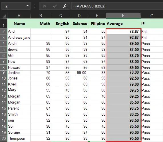
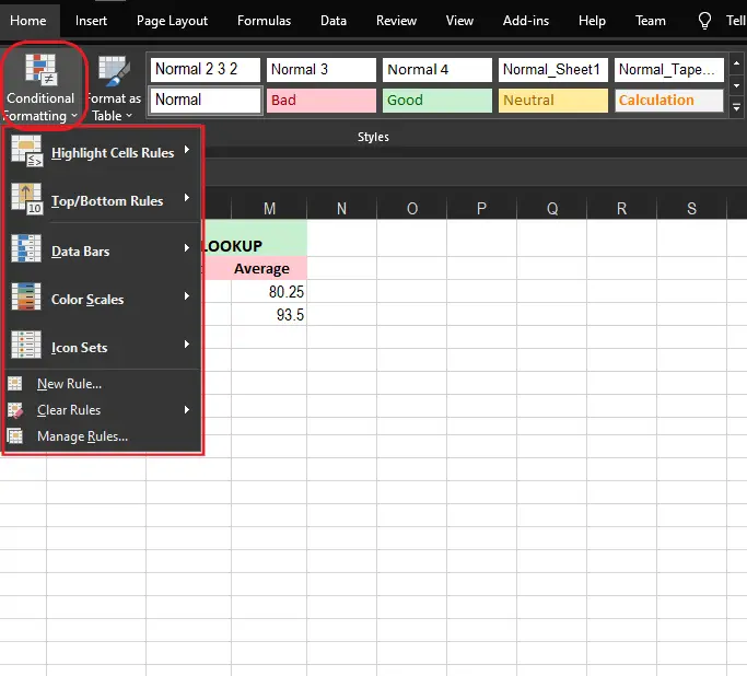
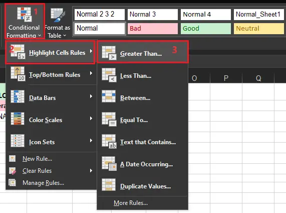
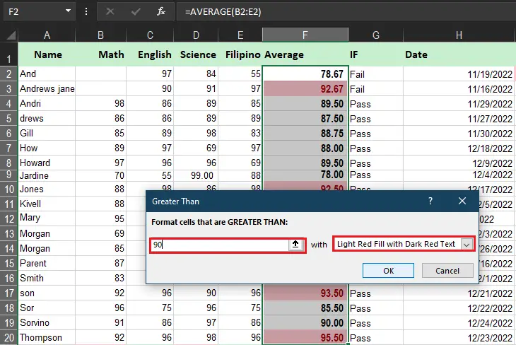
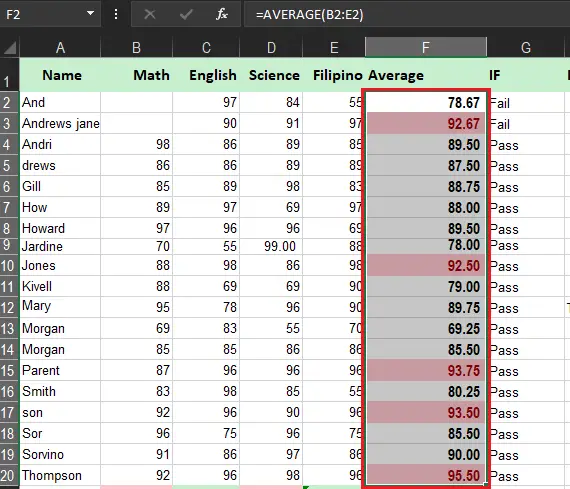
Take note can use any other rule depending on your option.

Greater than or equal to
Between two values
Text that contains specific words or characters
Date occurring in a certain range
Duplicate values
Top/bottom N numbers

Conditional Formatting Formula Excel

Take your Excel skills to the next level and use a formula to determine which cells to format. Formulas that apply conditional formatting must evaluate to TRUE or FALSE.

1. Select the range of cells you want to format using the formula. In our sample it’s G2:G20.

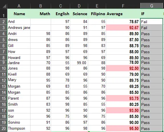
Range of cell for conditional formatting

2. On your worksheet Home tab, in the Styles group, click Conditional Formatting. Then when the dropdown list appears, Click New Rule.

New rule conditional formatting

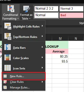
3. Select ‘Use a formula to determine which cells to format‘. Then enter the formula =G2:G20=”PASS”. After you select your preferred formatting rule and Click OK.

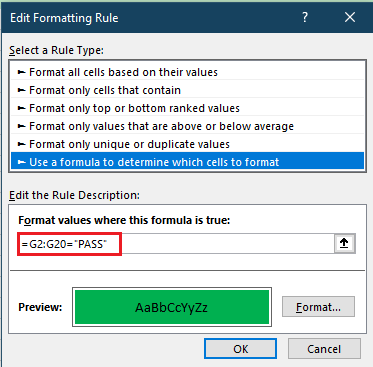
conditional formatting uing formula

4. Then the result of all the pass cells will be highlighted as Green.

New Rule using formula Result

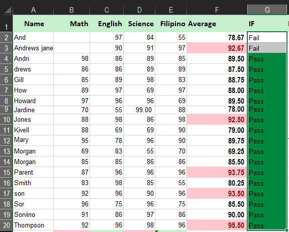
Excel Conditional Formatting Based on Another Cell

Using conditional formatting in your business logic or analysis does not limit you on a single rule only, actually you can add as many as you need.

For instance, you want all grades with a line of nine to be Yellow and a line of 8 to be green thus the line of 7 is red it will work. All you need to do is to specify them correctly.

If the “greater than 99” rule is placed first, then only the yellow formatting will be applied because the other two rules won’t have a chance to be triggered.

To re-arrange the rules, this is what you need to do:

Select any cell in your dataset covered by the rules.

Conditional formatting range

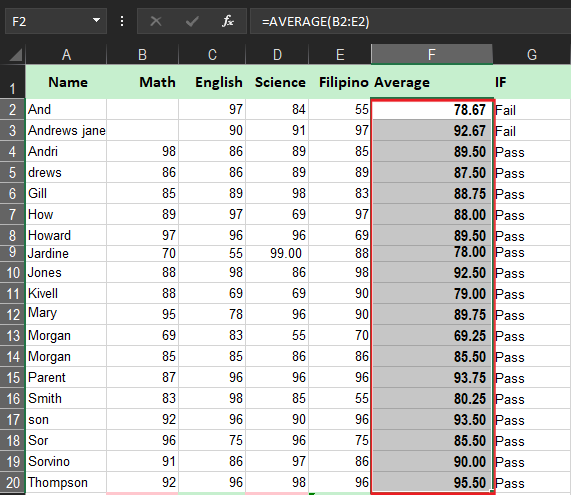
Open Conditional Formatting then Click Manage Rules… to proceed to Rules Manager.

Manage Rules

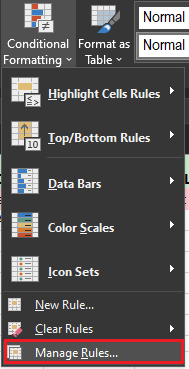
Click the rule that needs to be applied first, and then use the upward arrow to move it to the top. Do the same for the second-in-priority rule.

Organize conditions

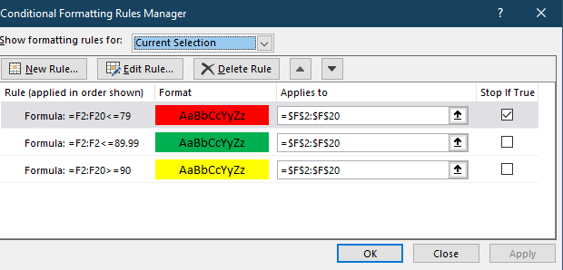
Select the Stop If True check box next to all but the last rule because you do not want the subsequent rules to be applied when the prior condition is met.

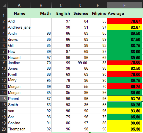
conditional formatting multiple conditions

Conditional Formatting Presets

Excel has several conditional formatting presets that will help you quickly apply to your data. Mainly it consists of three categories:

Data Bars: These horizontal bars are inserted into each cell, likely a bar graph.

Data bars

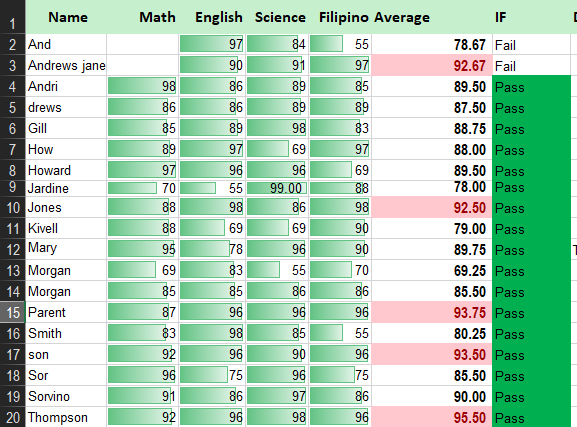
Color Scales: The color of each cell changes depending on the value. The color of the scale uses two or three gradients. For instance, on the Green-Yellow-Red color scale, the highest values are green, the average values are yellow, and the lowest values are red.

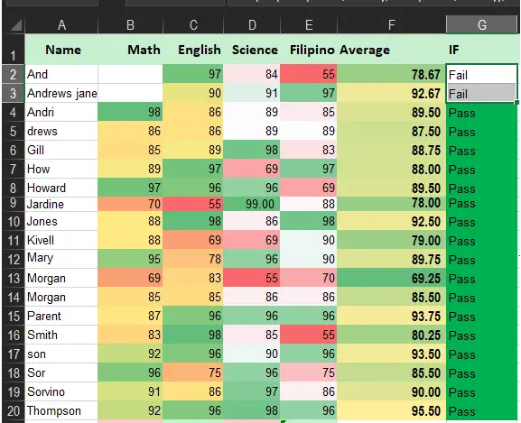
Color Scale conditional formatting

Icon Sets: It enters a specific icon on the cell based on its value.

Icon Sets Conditional Formatting

Summary

To sum up, this article about excel conditional formatting includes ways where to apply and examples that clarify the usefulness of conditional formatting.

If you have missed our other tutorials you can visit MS Excel tutorial for more.

See you on our next tutorial. Thank you for reading!

Источник

Spreadsheets are the go-to information hub for individuals, teams, and organizations of all sizes to store data. However, large data sets can make it difficult to identify trends, pick out key pieces of information, and track deadlines. Luckily, Microsoft Excel has a feature called conditional formatting that alleviates some of these challenges.

Conditional formatting enables you to apply special formatting to cells in your spreadsheet that meet certain criteria. Excel has a sizable library of preset conditions that you can apply fairly simply, or you can create your own conditional formatting rules using Excel formulas. This guide will provide in-depth step-by-step examples of the most popular conditional formatting functions for basic and advanced users in Excel 2016. Then, we’ll show you how to perform the same functions in another spreadsheet application, Smartsheet.

What Is Conditional Formatting?

Conditional formatting is a feature of many spreadsheet applications that allows you to apply special formatting to cells that meet certain criteria. It is most often used to highlight, emphasize, or differentiate among data and information stored in a spreadsheet.

Conditional formatting enables spreadsheet users to do a number of things. First and foremost, it calls attention to important data points such as deadlines, at-risk tasks, or budget items. It can also make large data sets more digestible by breaking up the wall of numbers with a visual organizational component. Finally, conditional formatting can transform your spreadsheet (that previously only stored data) into a dependable “alert” system that highlights key information and keeps you on top of your workload.

Originally a powerful feature of Excel, other spreadsheet applications have also adopted this functionality.

Conditional Formatting Basics

Conditional formatting consists of four main components: if-then commands, preset conditions, custom conditions, and applying multiple conditions. We’ve outlined how to use these commands and conditions to create and apply rules to your Excel spreadsheets below:

If-Then Logic: All conditional formatting rules are based on simple if-then logic: if X criteria is true, then Y formatting will be applied (this is often written as p → q, or if p is true, then apply q). You won’t have to hard-code any logic, though — Excel and other spreadsheet apps have built-in parameters so you can simply select the conditions you want the rules to meet. Advanced users can also apply the program’s built-in formulas to logic rules.
Preset Conditions: Excel has a huge library of preset rules encompassing nearly all functions that beginner users will want to apply. We’ll familiarize you with several of the most popular ones in the next section.
Custom Conditions: For situations where you want to manipulate a preset condition, you can create your own rules. If appropriate, you can use Excel formulas in the rules you write.
Applying Multiple Conditions: You can apply multiple rules to a single cell or range of cells. However, be aware of rule hierarchy and precedence — we’ll show you how to manage stacked rules in the walkthrough.

Overall, applying conditional formatting is an easy way to keep you and your team members up to date with your data — calling visual attention to important dates and deadlines, tasks and assignments, budget constraints, and anything else you might want to highlight. When applied correctly, conditional formatting will make you more productive by reducing time spent manually combing data and making it easier to identify trends, so you can focus on the big decisions.

How to Apply Basic Conditional Formatting in Excel

You can apply conditional formatting to your Excel spreadsheets using various tools and features found within the program. This step-by-step walkthrough shows you how to apply the most commonly used formatting for highlighting, data bars, color scales, and more.

Step 1: Apply Highlight Rules to Your Excel Spreadsheet

Highlight rules apply color formatting to cells that meet specific criteria that you define. They are the most basic type of conditional formatting rule, and Excel provides a variety of preset highlight functions.

Open an existing spreadsheet in Excel, or start from scratch and manually enter new data. In this example, we’re using an inventory list that tracks the number of each item currently in stock, as well as some additional information about each product.
To apply highlight rules, select the range of values you want to apply a rule to. For this example, we want to highlight any product that’s quantity is less than 100 units. So, select the values in the Qty. column (C4:C26).
From the Home tab, click Conditional Formatting on the right side of the toolbar, and click Highlight Cells Rules from the dropdown menu. Click Less than.
A box will appear. Type 100 in the empty field. Click OK.
Your spreadsheet will now reflect this highlight rule, with the quantities less than 100 highlighted red with red text.
Tip: You can change the color of the highlighted cell by clicking on the Format with: dropdown menu and selecting on another option.
To highlight text cells, repeat step 2. This time, we want to highlight certain model types (M compatible), so we’ll select the cells in the Item name column.
Click Conditional Formatting > Highlight Cells Rules > Text that Contains…
Type M compatible in the text box. To differentiate from our previous highlight rule, select green fill with dark green text from the Format with: dropdown menu. Click OK.
Now, cells containing the text M compatible are highlighted.

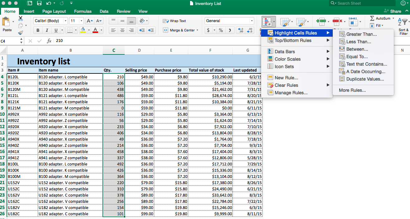
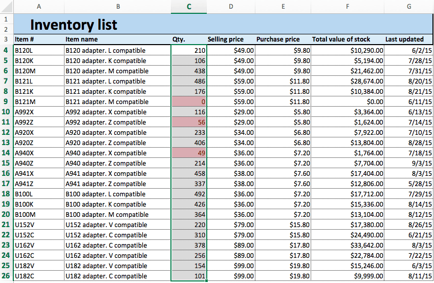
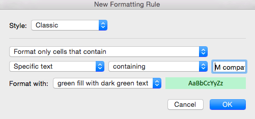
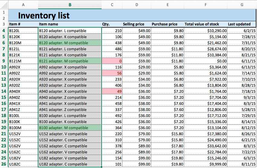
Using these same steps and menu options, you can apply highlight rules to find Duplicate Values, Dates, or values that are Greater than…, Equal to…, or Between… values that you select. All of these possibilities are available through the menu options.

Step 2: Create Top/Bottom Rules

Step 3: Apply Data Bars

Data bars apply a visual bar within each cell. The length of the bar relates the value of the cell to other cell values in the selected range.

We’ll apply data bars to the Qty. column so we can easily assess the ratios of items in stock. Click the top of the Qty. column to select this range of cells.
Click Conditional Formatting > Data Bars. You’ll see two options — one for Gradient Fill and one for Solid Fill. They function identically; just select the option and color you prefer.
Your sheet will now reflect the added rule.

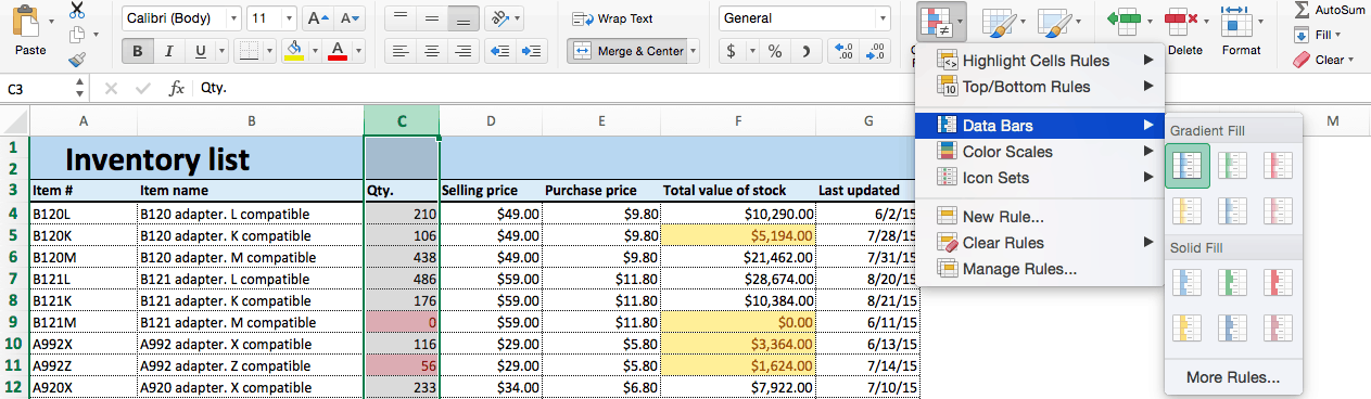
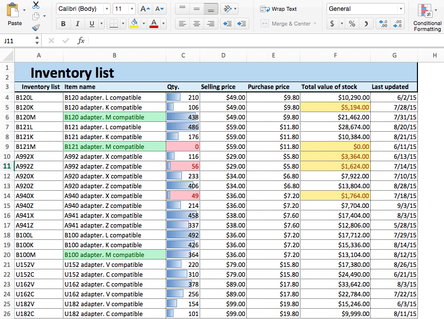
Step 4: Apply Color Scales

Color scales are similar to data bars in that they relate a cell’s values in a selected range. However, instead of representing this relationship by the length of a bar, color scales do so with color gradients. One color is assigned the “lowest” value and another the “highest,” with a range of colors in between.

We’ll apply color scales to our Selling price column. Click the top of column D to select this range.
Click Conditional Formatting > Color Scales. You’ll see a variety of different color ranges; select the one you want.
Your spreadsheet now shows the selling prices by color — red cells are the most expensive, and green cells are the least expensive.

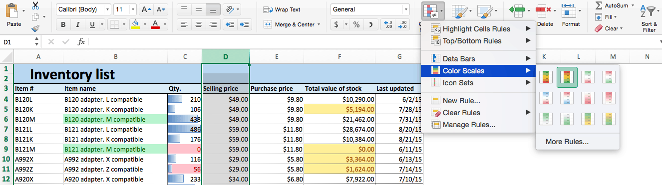
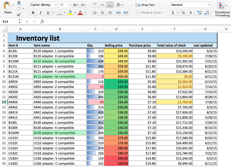
Step 5: Apply Icon Sets

Icon sets apply colorful icons to data. They are simply another way to call attention to important data, and relate cells to one another.

We’ll apply icon sets to the Purchase price column to show low, middle, and high priced items. Click the top of the Purchase price column to select the range of values.
Click Conditional Formatting > Icon Sets. You’ll see a variety of options for Directional, Shapes, Indicators, and Ratings icons. You can choose any of these to fit the needs of your data. In this example, we’ll choose the first Directional option: red, yellow, and green arrows that indicate high, middle, or low priced items.
Your sheet reflects this new formatting rule.

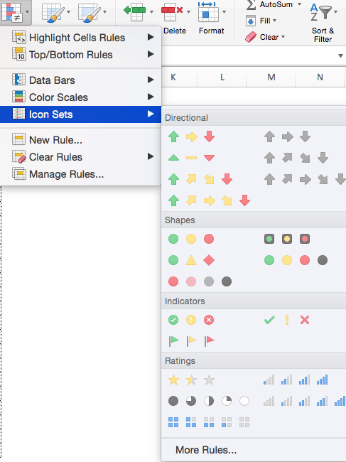
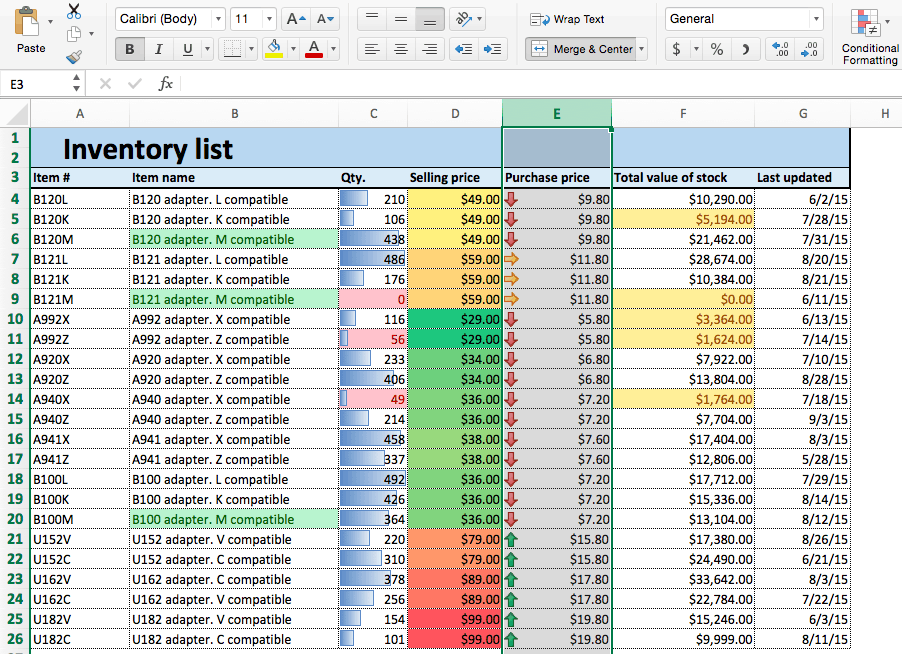
Step 6: Edit and Delete Conditional Formatting Rules

Now you’ve learned the most common conditional formatting presets in Excel, your spreadsheet provides a lot of information at a glance. However, you might want to edit some of these rules later on, or delete them completely.

Click Conditional Formatting and select Manage Rules… from the dropdown list.
The Manage Rules box will appear. Click the dropdown menu at the top of the box and click This Sheet to list the conditional formatting rules you have applied to the current sheet.
To edit a rule, click the rule you want to change. In this example, we want to highlight the bottom ten values in the Total value of stock column, rather than the bottom five that we currently have highlighted. Click the Bottom 5 row. Then, click Edit Rule… at the bottom of the box.
A new box opens where you can adjust the conditions of the rule. Type 10 in the number field and click OK.
Excel will bring you back to the Manage Rules box. You must click OK to save the changes you made to the original rule.
To delete a rule, return to the Manage Rules box and choose This Sheet. Click the rule you want to delete — in this case, the color grading on Selling price. Click the — symbol (next to Edit Rule…) in the lower left hand corner. Click OK.
The conditional formatting on the Selling price column is now deleted.

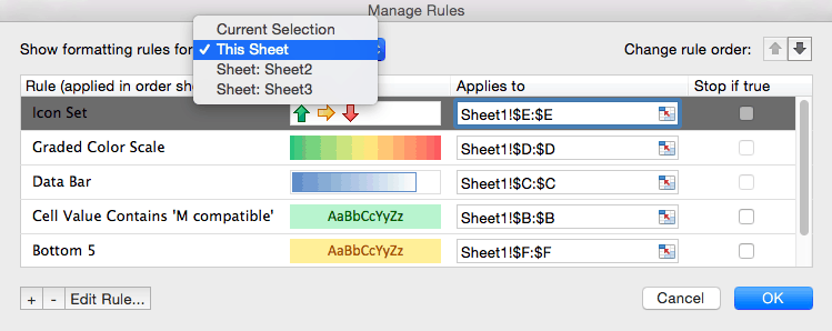
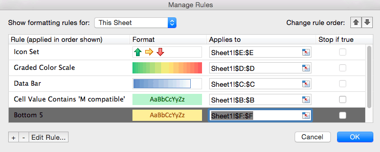
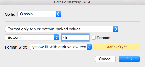
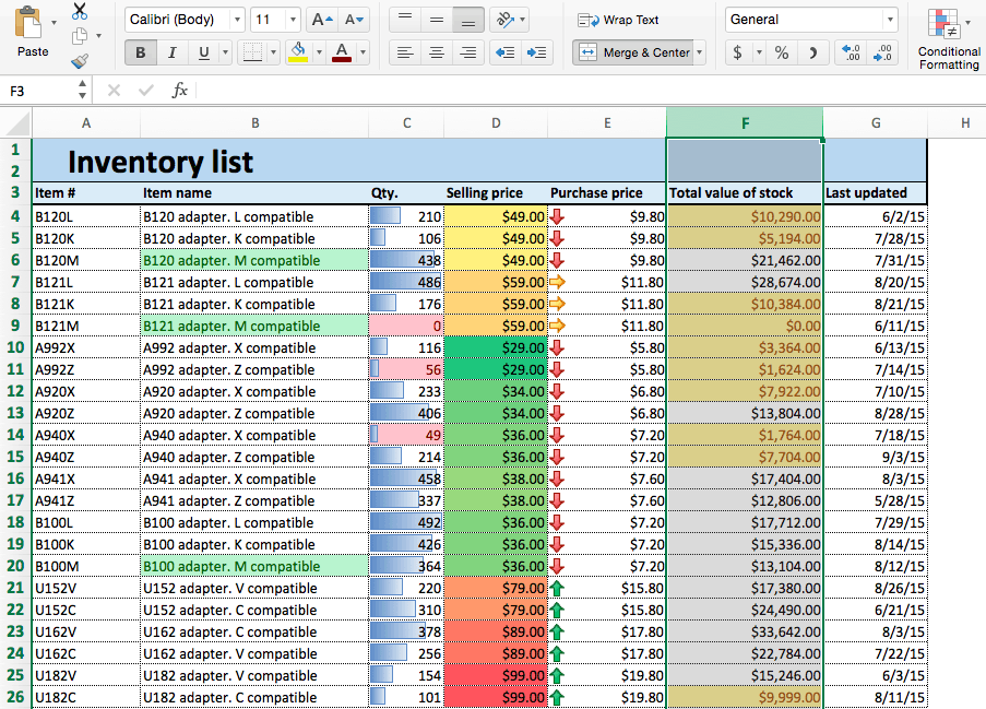
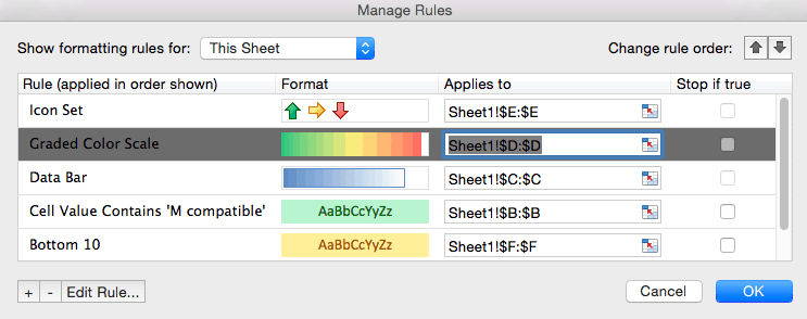
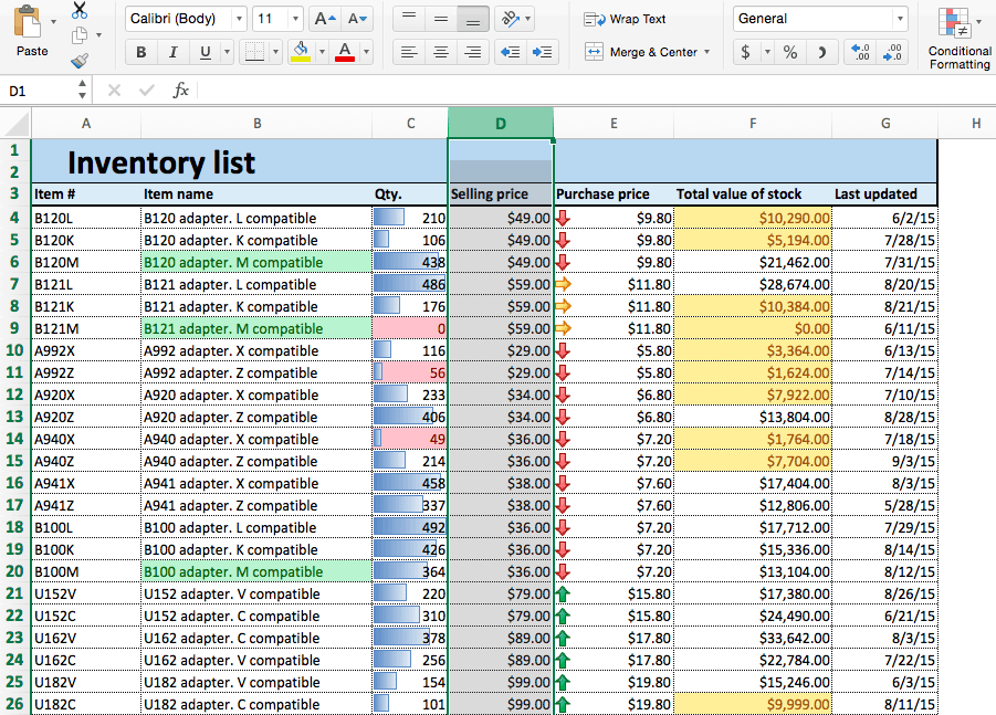
You now have everything need to create basic conditional formatting using presets in Excel 2016. For more advanced functionality such as creating a new rule, using Excel formulas, and creating rules dependent on another cell, see the “Advanced” section below.

First, we’ll look at how we can apply the same conditional formatting rules we learned in Excel to another spreadsheet program, Smartsheet.

How to Apply Basic Conditional Formatting in Smartsheet

Use conditional formatting in Smartsheet to apply many of the same rules and effects available in Excel. We’ll guide you through every function described in the previous section, with some modifications that better align with Smartsheet features.

You can create spreadsheets in Smartsheet two ways: by manually entering data into Smartsheet, or by importing an existing spreadsheet from programs like Excel and MS Project. For this tutorial, we’ll use the same data set from the Excel tutorial, so we’ll import the original version (with no conditional formatting) from Excel.

Step 1: Open Your Existing Excel Spreadsheet in Smartsheet

Step 2: Apply Highlight Rules

To highlight a cell, click the conditional formatting icon on the toolbar.
A box will appear where you can set conditional formatting rules. Click Add New Rule in the top left corner. The if-then logic is already written into the new rule, so you can simply create the conditions.
Click set condition. Just like in the Excel example, we want to highlight any items that are stocked below 100 units. Select Qty. from the column list on the left, select is less than from the center dropdown list, and then type 100 in the field on the right. Click OK.
Now we need to apply the formatting. Click this format and a dropdown menu with formatting options appears. For this example, we’ll use a paint fill. Click the paint bucket icon and select red.
Specify which cells should get this formatting. Smartsheet will default to format the entire row, but we only want to highlight the cells in the Qty. column. Click entire row and click Qty. from the dropdown list. Click OK.
Your conditional formatting rule is now reflected in your spreadsheet.
To highlight text cells, repeat steps 1 and 2. Click set condition. Now, we want to highlight any M compatible items. Select Item name from the left-most list, contains from the center list, and type M compatible in the right field. Click OK.
Click this format and click the paint bucket item. Select green. For this rule, we want to highlight the entire row. (Again, Smartsheet defaults to this option.) Click OK.
Your second rule is now reflected in your data set.

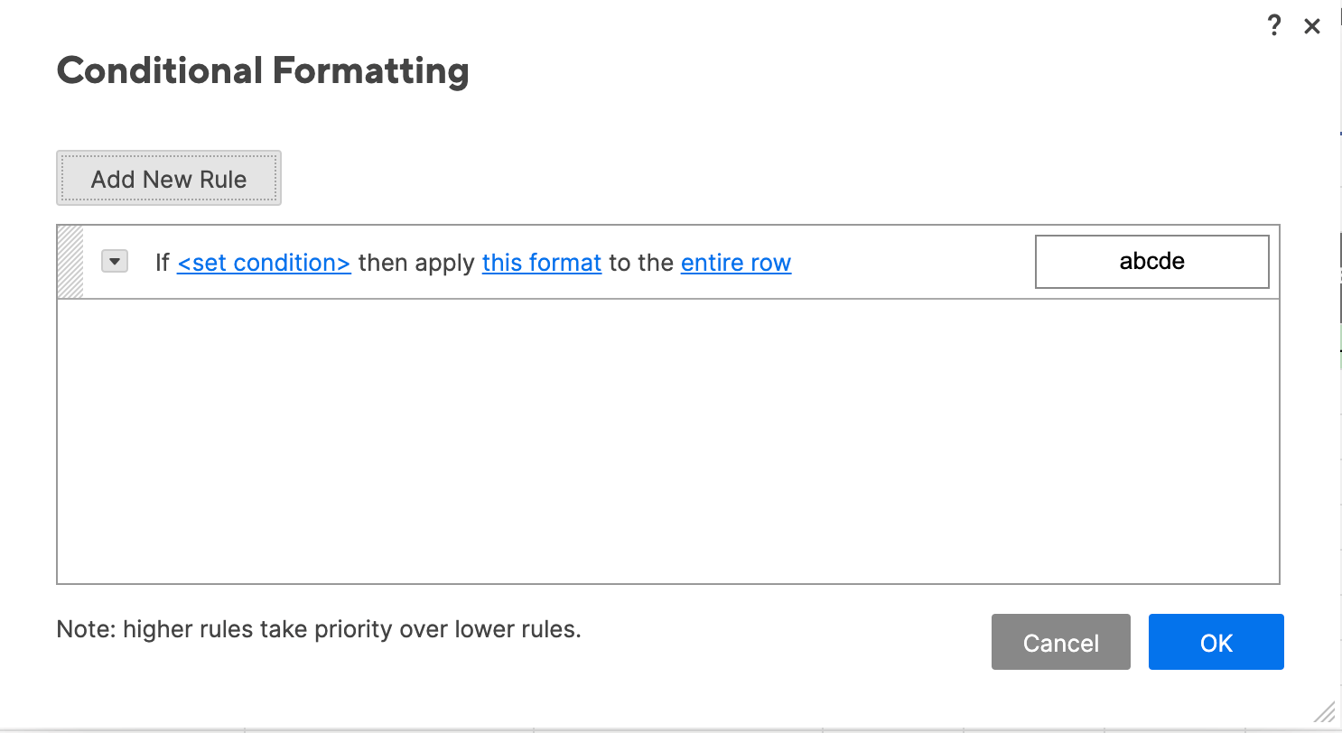
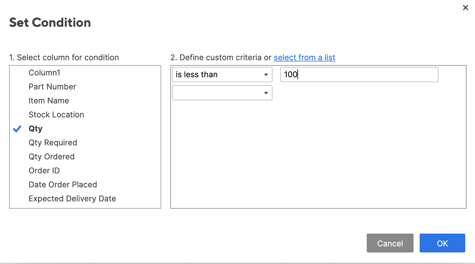
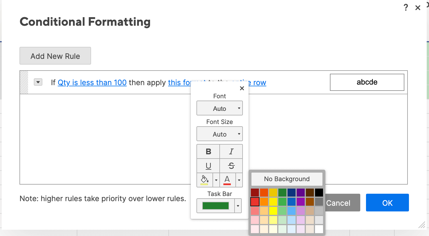
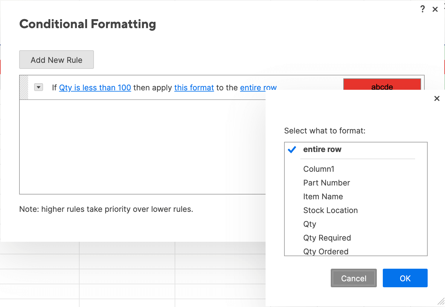
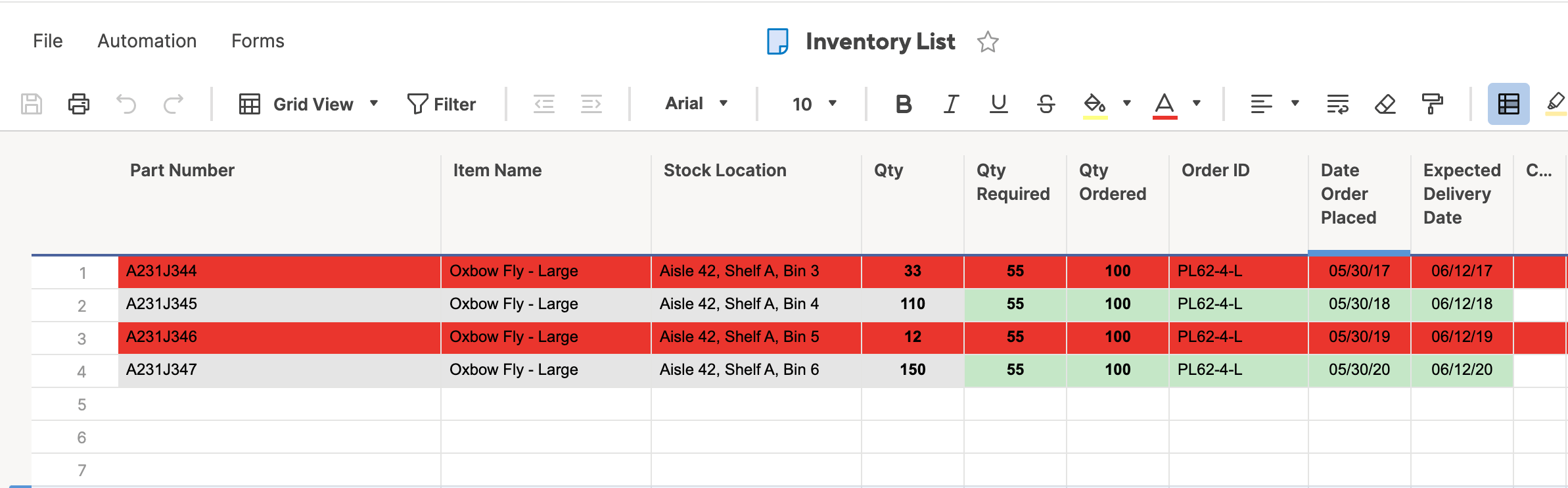
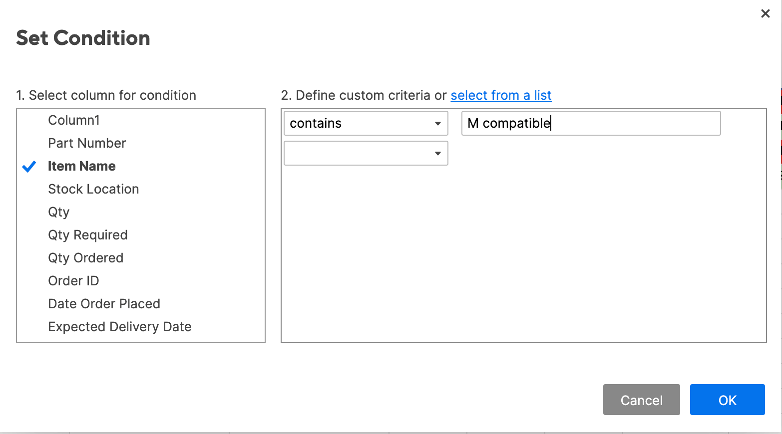
Step 3: Apply Progress Bars (Data Bars)

In place of Excel’s Data Bars preset, you can create Progress Bars in Smartsheet. Progress Bars are a symbol that you can apply to cells to show and compare the level of completeness. In this example, we’ll apply progress bars to denote current inventory levels (from zero to 100 percent).

To create Progress Bars in Smartsheet, you first need to create a new Symbols column. Cells in a Symbols column will only hold special characters, such as progress bars.
To create a new column, right-click the Qty. column and click Insert Column Right.
A box will open. We’ll name this column Inventory Level, and select Symbols… from the list of column-types. In the right-hand field, scroll down and select the progress bar icon. Click OK.
Click into cells in the new Inventory Level column and select the appropriate level of inventory: Empty, Quarter, Half, Three Quarter, or Full. This progress bar relates the current level (from the Qty. column) to level you need.
Here’s what your sheet will look like when all progress bars are filled in.

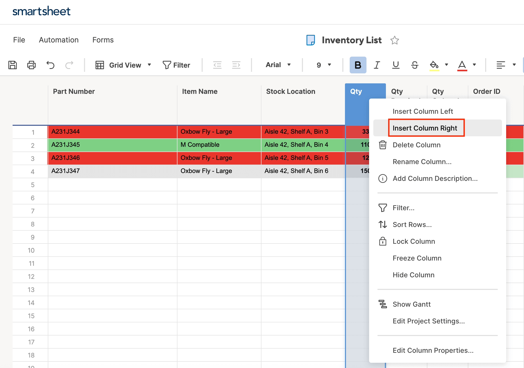
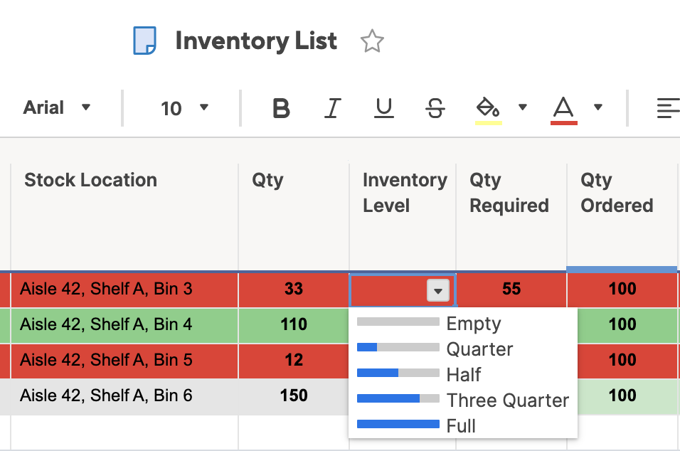
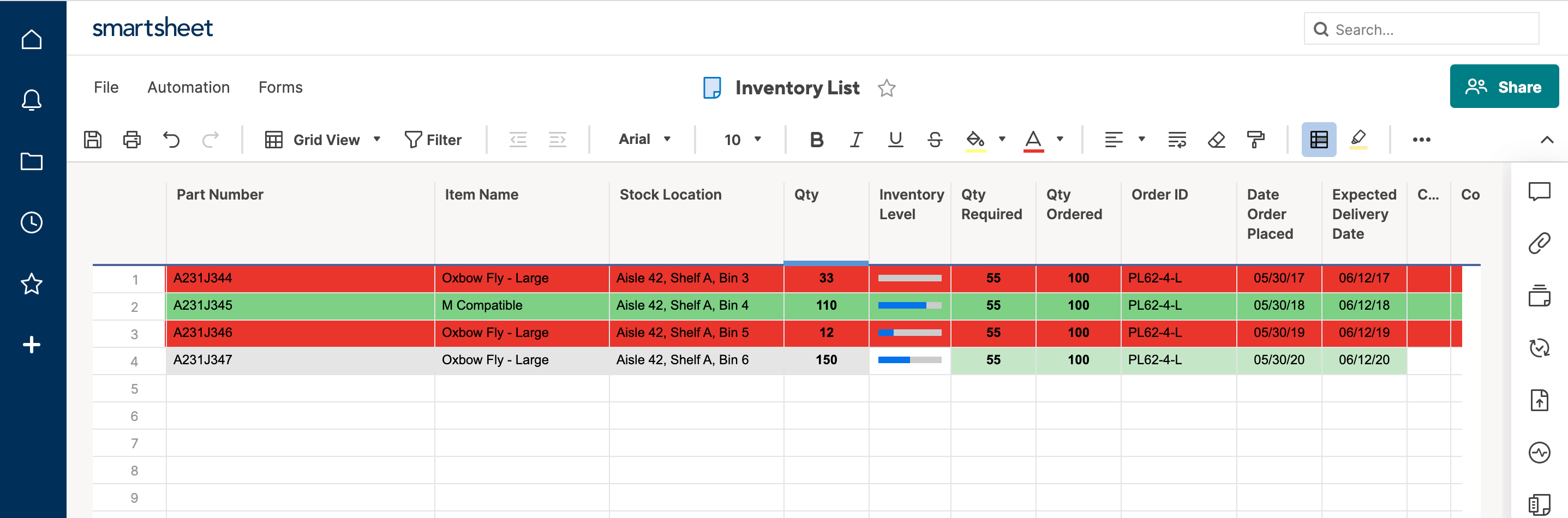
Tip: You can also type Empty, Quarter, Half, Three Quarter, or Full into each cell, and Smartsheet will autofill with the appropriate progress bar.

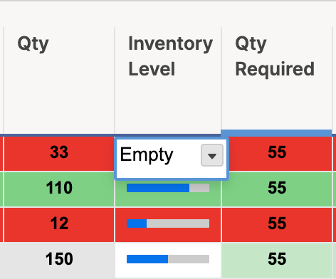
Tip: You can also automate progress bars by using an if-then formula in Smartsheet. For more information on how to do this, check out this resource on symbol formulas.

Step 4: Apply Icon Sets

To apply icon sets in Smartsheet with conditional formatting, you’ll have to use formulas (we’ll get into that in the “Advanced” section). Instead, you can add informative icons to your data by creating a special Symbols column.

Right-click the Qty. column and click Insert Column Right.
In the box that opens, type Qty. Status in the name field. Click Symbols from the dropdown menu and choose from the library of available symbols (Flag, Priority, Decision, Status, Direction, and Measure icons). In this example, we’ll choose RYG balls in the Status section. Click OK.
Now, you can update your sheet with the appropriate color status ball by adding conditional formatting as shown above.

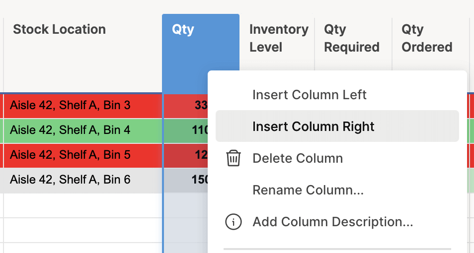
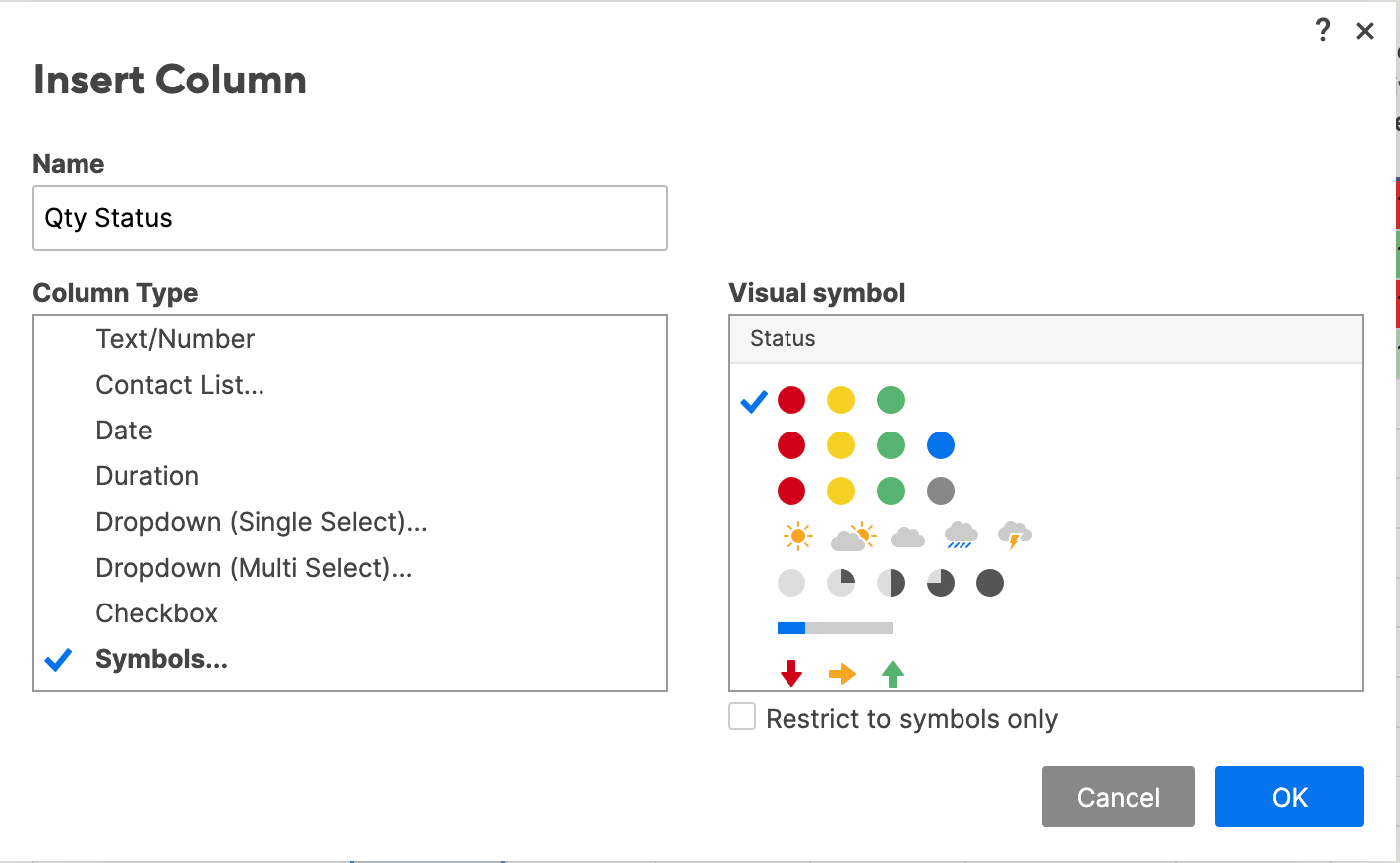
Step 5: Edit and Delete Conditional Formatting Rules

Editing and deleting conditional formatting rules in Smartsheet is extremely easy.

To edit a rule, click the Conditional Formatting icon on the toolbar to open the list of rules. Click the condition you wish to change and edit the information in the box that opens. Click OK.
To delete a rule, click the carrot on the left side of each rule. Click Delete Rule from the dropdown menu. Click OK.

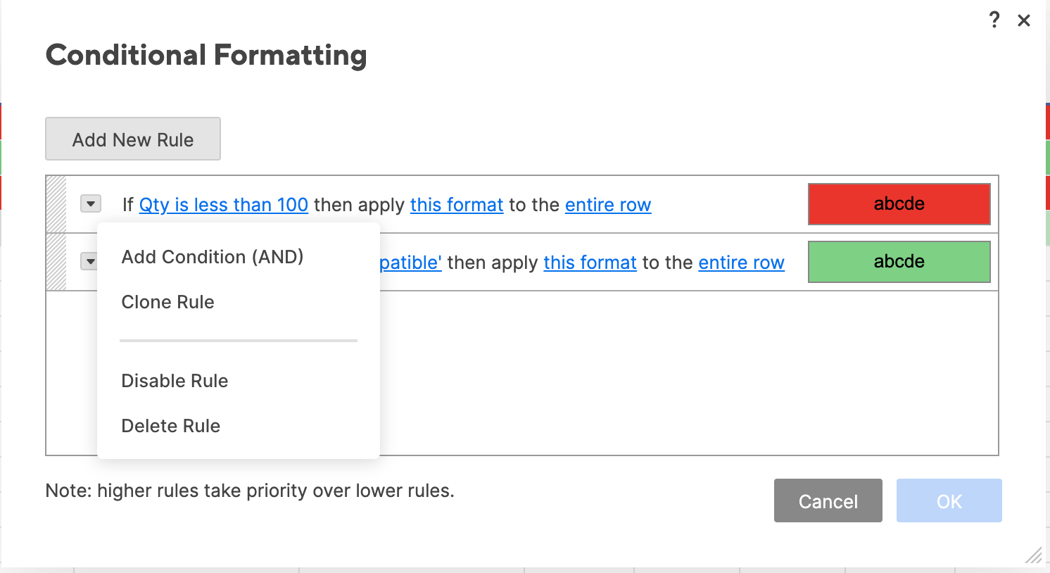
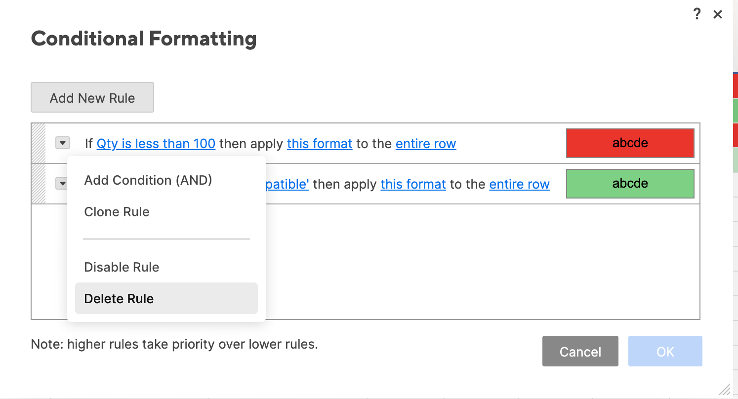
Tip: You can also disable a rule by clicking Disable Rule from the dropdown menu and then clicking OK. This will put the rule on “hold” without deleting it, in case you want to re-enable it later on.

Now you know how to use conditional formatting and other colors and symbols to add formatting to your sheet in Smartsheet. In the following sections, we’ll walk you through more advanced conditional formatting functions in Excel and Smartsheet.

Advanced Conditional Formatting Functions in Excel

Once you have mastered the basics, Excel includes some additional advanced conditional formatting functions. We’ll guide you through applying stop-if-true rules, using the AND formula, setting rule hierarchies and precedence, and other unique situational formatting conditions below.

Step 1: Create a New Rule and Apply Stop if true Rule

In some instances, you might want to stop a certain condition, without deleting the entire rule. The Stop if true rule in Excel enables you to do so.

In our example, we applied an icon set of three directional arrows to the Purchase price column to indicate low, medium, and high price ranges. However, we might actually only want to call attention to the lowest cost items, as three icons can clutter the sheet (and provide more information than actually needed).
First, create a separate condition on this column. Click the Purchase price column to select these values.
Click Conditional Formatting > Manage Rules… to open the Manage Rules box. Keep the default Show formatting rules for: Current Selection from the dropdown menu, because we are only adjusting the rule on this column.
Click the + in the bottom left corner to create a new rule. A new box opens where you can assign conditions to the new rule.
From the Style menu, select Classic.
Instead of applying a different icon to bottom, middle, and top price ranges (as we currently have), we only want to show the bottom 50 percent. So, select Top from the left dropdown menu, type 50 in the middle field, and check the Percent box.
To apply color formatting, Select Custom format from the Format with dropdown menu, and a new formatting box opens. Click the Fill tab, and click No Color.
Next, click the Font tab, and select black text. Click OK.
Click OK again in the original New Formatting Rule box.
You’ll return to the Manage Rules box, where you now have two rules applied to the Purchase price column. Click the Stop if true box to the right of the new rule you just created. Click OK.
Your sheet will now only show the icon sets for the items with a purchase price in the bottom 50 percent.

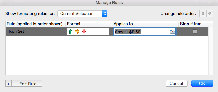
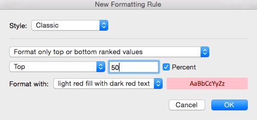
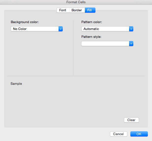
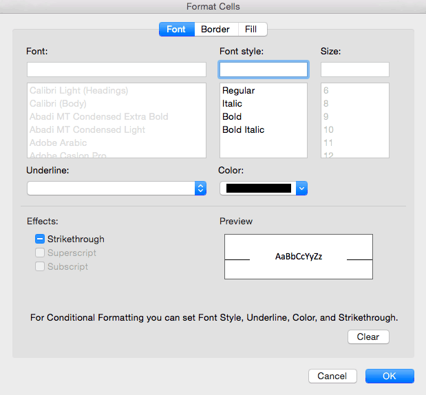
Step 2: Apply Multiple Conditions to a Rule with AND Formula

Adding Excel’s formulas to your conditional formatting rules is one way to elevate your logical rules. The AND formula is one of the most popular, easy-to-use formulas. It lets you add multiple conditions within a single rule, rather than writing out each rule separately. To format cells they must meet both conditions.

We’ll create a new rule to highlight any cell in the Item # column that contains both a B and an L. Click the top of the Item # column to select this range of cells.
Click Conditional Formatting > New Rule.
In the dialogue box, select Classic from the top dropdown list. Select Use a formula to determine which cells to format, since we’re using a formula.
We want to search cells in the Item # column for a B and L, and highlight that cell when both conditions are true. To do this, we’ll use Excel’s ISNUMBER and SEARCH formulas, with the AND formula, to look for the B and L values.
=AND(ISNUMBER(SEARCH(«B»,A1)),ISNUMBER(SEARCH(«L»,A1)))
Click OK. Your sheet will highlight all cells in Item # that meet both of these conditions.

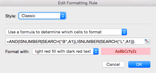
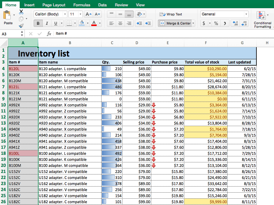
Tip: Understanding the formula:

We use AND at the beginning of the formula to show that both of the following conditions must be met in order to apply the conditional formatting.
The basic syntax of the nested formula is ISNUMBER(SEARCH(“substring”,text)) where “substring” is the character(s) you are looking for, and “text” is the cell(s) you want to search.
We are searching for two separate conditions, so we write the ISNUMBER(SEARCH(“substring”,text)) formula twice, separated by a comma.

This example is just one of hundreds of different formulas you could enter with the AND function. For more information on using Excel formulas with conditional formatting, click here.

Step 3: Conditional Formatting Based on Another Cell

You can also create rules to highlight certain cells based on the value of another cell.

In this example, we’ll create a “quantity threshold” — items with inventory level below this threshold will be considered “at risk.” We already have a rule that highlights cells in the Qty. column under 100. However, that threshold might change over time, depending on manufacturing or selling rates. So, we want to create a highlight rule that is dependent upon a threshold that we set.
To the right of your data, create a box for Quantity Threshold and choose an amount. In this example, we use 200. (Note the cell you type the amount in. Here, it’s I5.)
Create a new rule by clicking Conditional Formatting > New Rule.
In the dialogue box, click Classic and Use a formula to determine which cells to format from the dropdown menus.
In the formula field, type =C4<$I$5 and keep the default formatting. Click OK.
Numbers in the Qty. column that are less than the Quantity Threshold in I5 (200) will now be highlighted.
Now, you’ve created a dynamic rule. This means that as your threshold changes, the rule will still be applied to the Qty. column and the formatting will adjust as appropriate.

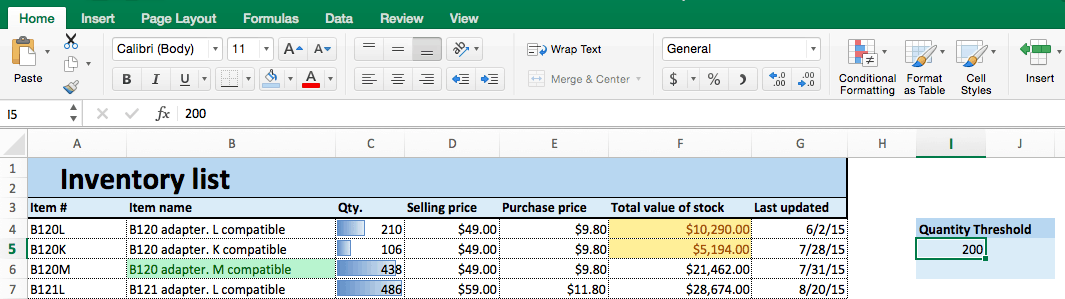
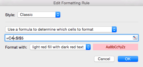
Tip: Understanding the formula:

In this formula, we are simply testing whether or not values in column C are less than the value in I5.
Start with “=C4” to tell Excel where we want to start evaluating values from.
Use ‘$’ symbol around I because it’s an absolute value — we are only evaluating cells in column C against this single cell.

Step 4: Data Validation and Dropdown Lists

While data validation is not technically monitored through conditional formatting rules, you can use it to a similar effect: controlling the formatting of your sheet. You can apply data validation to ensure that any cell-type only allows certain entries (text or numbers only, text length, etc.). In this example, we’ll show you how to create a dropdown list and validate data only from that dropdown list.

We’ll create an additional column of which employee last updated the sheet, and create a dropdown list to choose from. First, click where you want to add the column on the sheet. Create a new column by clicking Insert > Insert Sheet Columns from the ribbon on the Home tab.
We’ll name this column Updated By.
Now we need to make a list of employees, that the dropdown list will later pull from. Create a second sheet (in the same Excel workbook) by clicking the + sign on the tab at the bottom of the spreadsheet, and write a list of employee names in column B.
Select the range of data (all the names) you want to include in your list. Make this list into a table by clicking the Insert tab > Table.
The dialogue box will show the range of data you selected for the table. Click My table has headers, since we began the list with Employees. Click OK.
Now we have to name this list so that Sheet 1 can pull from it. Click Formulas tab > Define Name on the ribbon.
In the dialogue box, type the name of the list. We’ll call it Employees. Double check that the selected range is still correct. Click OK.
Go back to Sheet 1. Now, we have to make the Updated By column into a dropdown list. We’ll use the data validation function to do this.
Select the Updated By column to apply data validation to this range of cells.
Click the Data tab on the ribbon and click Data Validation > Data Validation…
In the dialogue box, choose List from the dropdown menu to restrict data entered in this range to a list. Type =Employees in the Source field, since we’re pulling from the list we just created (in Sheet 2). Click OK.
There is now a dropdown list in the Updated By column. Your sheet will only accept data in this column that comes from the Employees list on Sheet 2.
You can now fill in the column by selecting a name from the dropdown list.

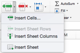
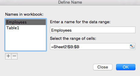
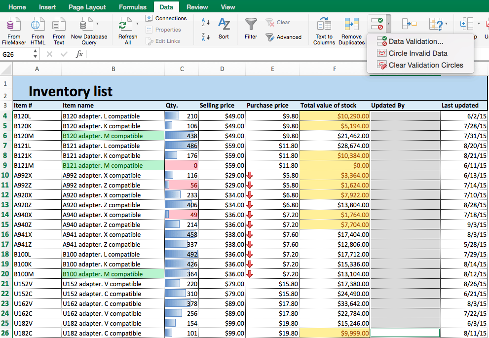
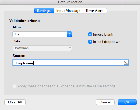
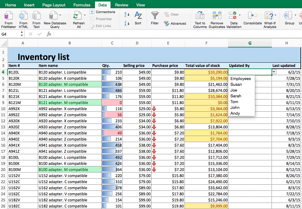
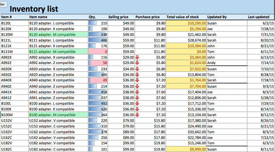
Step 5: Rule Hierarchy and Precedence

As you accumulate conditional formatting rules, watch out for rule hierarchy. Since you can apply multiple conditions to a cell (or row), they occasionally conflict. When this happens, Excel has default precedence rules that may cause one rule to override another, so you can lose your formatting. To combat this, you can change the hierarchy of the rules.

Adjusting rule hierarchy in Excel is straightforward, but you should also understand the logic behind rule precedence:

Newer rules will always assume precedence over older rules. This means that the precedence of your rules will be in the reverse order of how you created them.
When multiple rules evaluate as true to a cell, they may or may not conflict. Applying multiple rules to a cell does not necessarily mean that they will interfere.
Rules don’t conflict if they are changing different things about the cell. For instance, if one rule changes text color and another changes fill color both rules should co-exist in the cell.
Rules conflict when the outcomes are the same. For instance, if one rule changes a font color to green and another changes the font color to blue the newer rule takes precedence.

To adjust rule hierarchy in Excel, follow these steps:

All rule hierarchy is controlled through the Rule Manager in Excel.
From the Home tab, click Conditional Formatting > Manage Rules… to open the Rule Manager.
Select This Sheet from the top dropdown list to pull up all lists applied to the current sheet.
To change the order (hierarchy) of rules, select a rule and click the up and down arrows in the top right corner to move it. Click OK. Remember the rule closest to the top will take precedence.

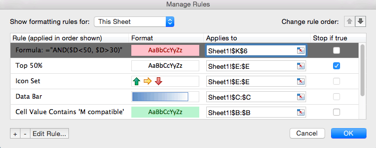
Advanced Conditional Formatting in Smartsheet

Many advanced Excel conditional formatting options are available to Smartsheet users, as well. We’ll teach you how to apply stop-if-true rules, create rules with multiple conditions, create formatting rules based on other cells, and set rule hierarchies and precedence.

Step 1: Add New Rule and Apply Stop If True Function

Adding a new rule in Smartsheet is easy (you already learned how in the “Basic” section). Now, we’ll apply the same “stop if true” logic from Excel in Smartsheet.

Add a new rule by clicking the conditional formatting icon on the toolbar. Click Add New Rule and click Set condition.
For this rule, we want to call attention to the shipment order dates that are after 06/20/30. The easiest way to do this is to apply the same logic as “stop if true” in Excel.
Click Shipment Order Date in the left field to set a condition in this column.
Instead of defining criteria (as we have been doing), click select from a list. The list of values in the Shipment Order Date column appear.
Click 06/20/30. Then, because we want to highlight all the dates that are not this date, check the Apply format when this condition is NOT met box. (This functions just like the “stop if true” box in Excel.) Click OK.
Click this format and apply whatever format you want. We’ll make the text bold.
Click entire row and select the Shipment Order Date column. Click OK.
Now, all dates other than 07/01/15 will be bolded in the Shipment Order Date column.

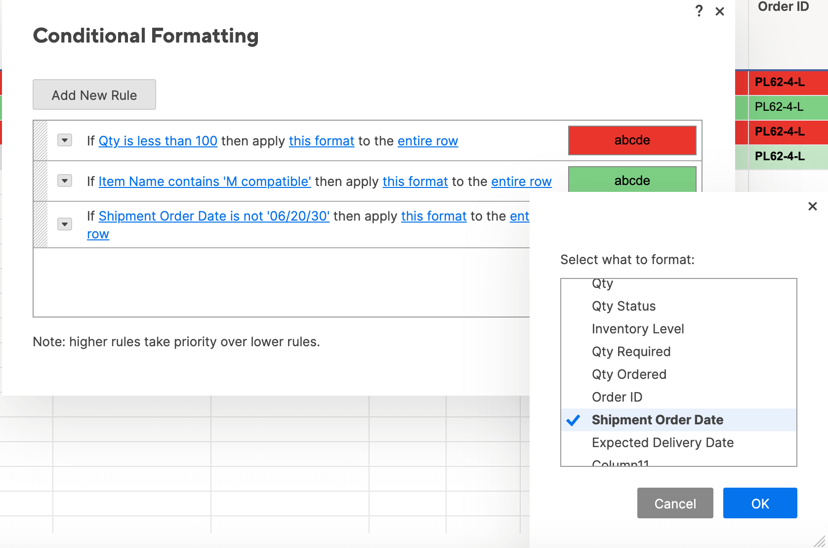
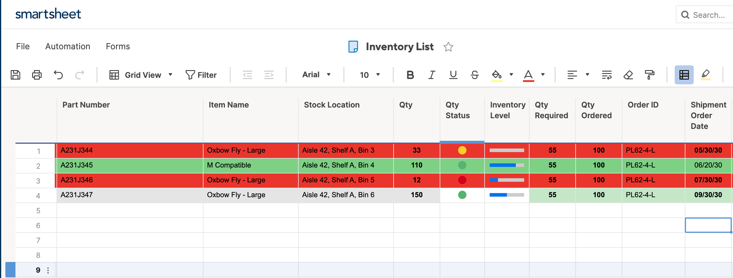
Step 2: Add Multiple Conditions to a Rule

Just like in Excel, you can use Smartsheet’s built-in formulas when creating conditional formatting rules. However, Smartsheet makes it easy to perform some of the simple functions that basic Excel formulas provide, so you don’t have to worry about remembering complicated formula syntax. To perform the AND function, you can simply click to add multiple conditions to any conditional formatting rule.

Click the conditional formatting icon on the toolbar and click Add New Rule.
Click set condition. We want to highlight cells in the Item # list that contain both a ‘B’ and an ‘L.’ Click Item # from the dropdown list on the left.
For the conditions, select contains and type B. Click into the second prompted condition and type L to create the second condition. (This will perform the AND function.) Click OK.
Apply the formatting to your rule. We’ll use a yellow fill.
Change entire row to Item #. Click OK.
Your sheet will now highlight those values in Item # that contain both a B and an L.

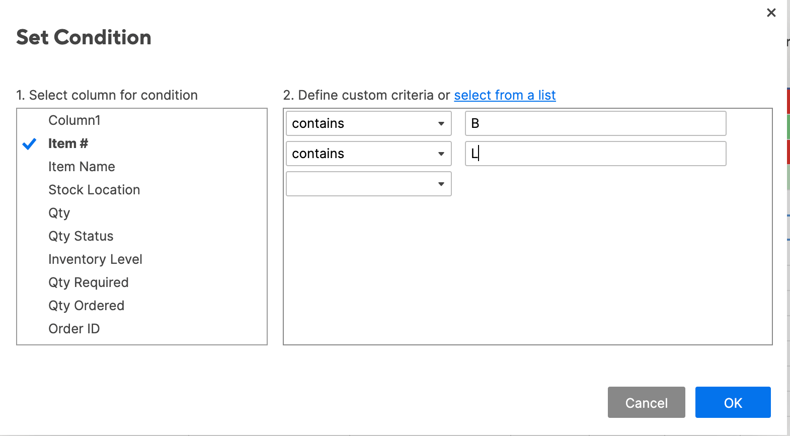
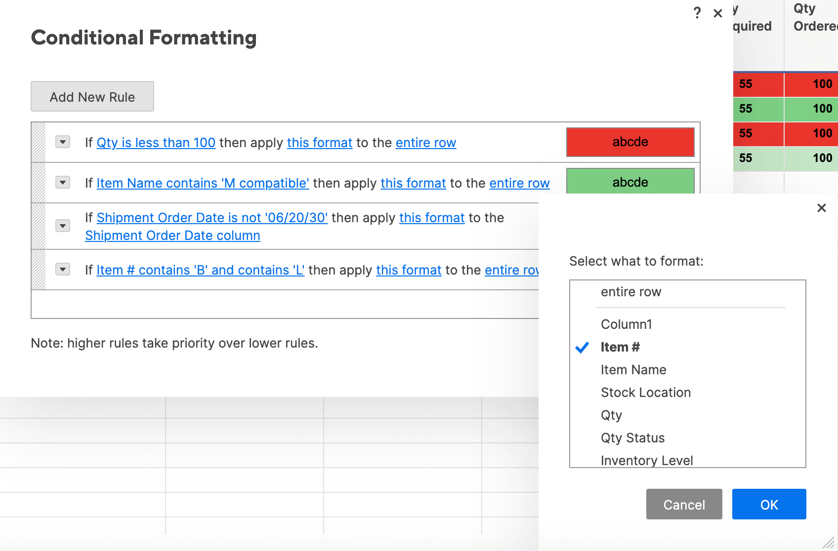
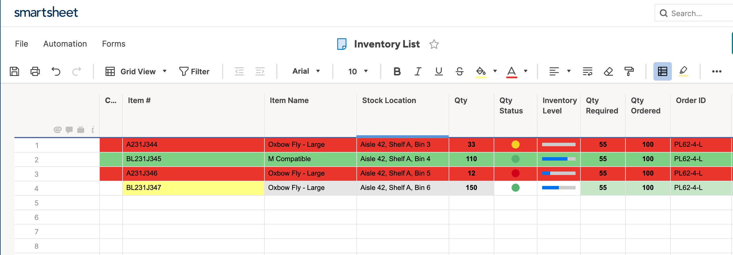
You can still use formulas with conditional formatting, if you’d like. For an introduction on how to use formulas, check out this resource.

Step 3: Conditional Formatting Based on Another Cell

Smartsheet also makes it easy to apply conditional formatting based on another cell. Instead of using complicated formulas to reference different cells, you can simply control which cells to pull from and format with a few clicks.

In this example, we want to highlight the Item Name column if the status bar is red, to call attention to at-risk items. To do this, we’ll create a rule that pulls from the Qty. Status column, but applies formatting to the Item Name column.
Click the conditional formatting icon on the toolbar and click Add New Rule > set condition.
Click Qty. Status from the drop down list and click Red. Click OK.
Apply a light red paint fill to format with.
Click entire row and select Item name. This will apply formatting to cells in the Item name column, even though we’re pulling information from the Qty. Status column.
Click your new rule and drag it to the top of your rules list. Since we have multiple highlighting rules, this will ensure that this rule takes precedence over others.
Cells in Item Name will now be highlighted if the Qty. Status ball is red.

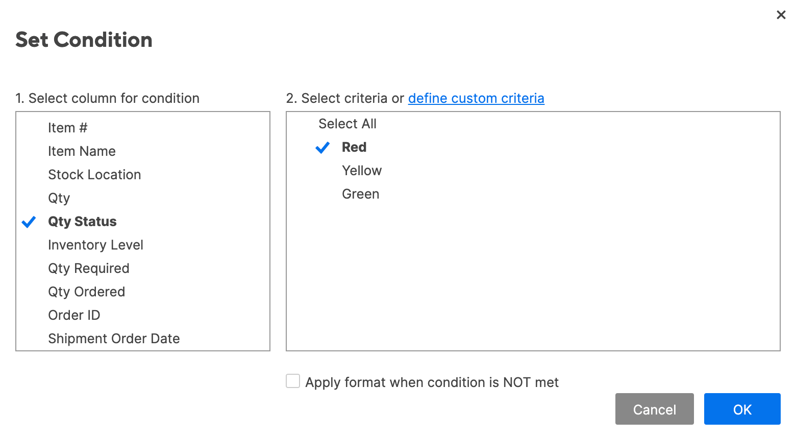
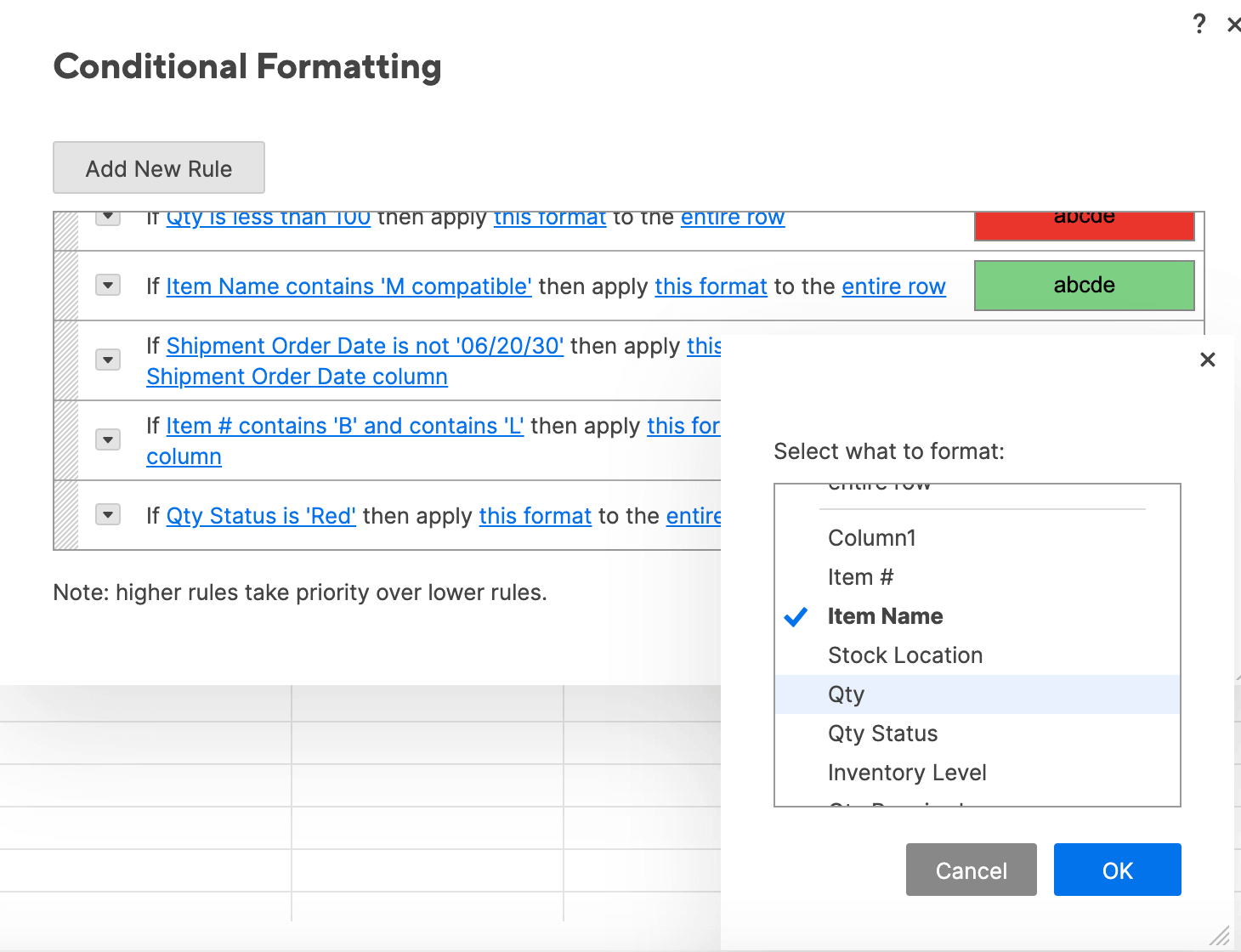
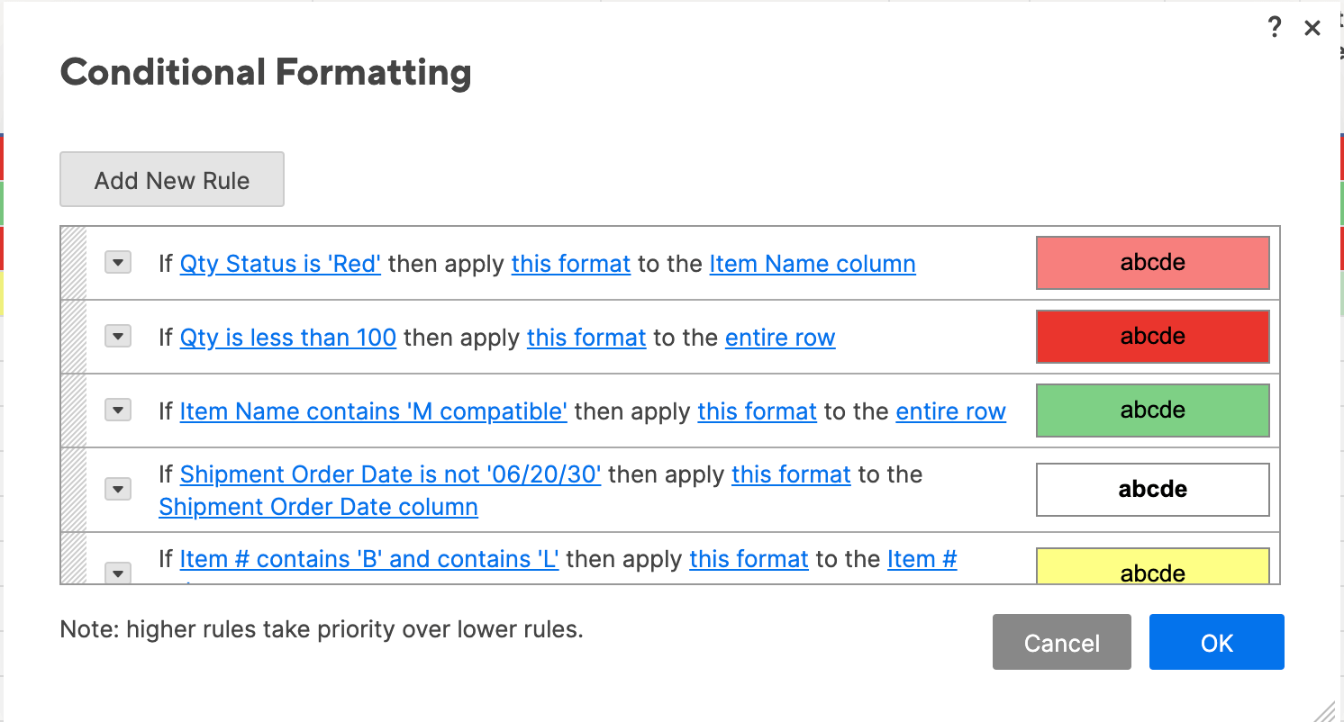
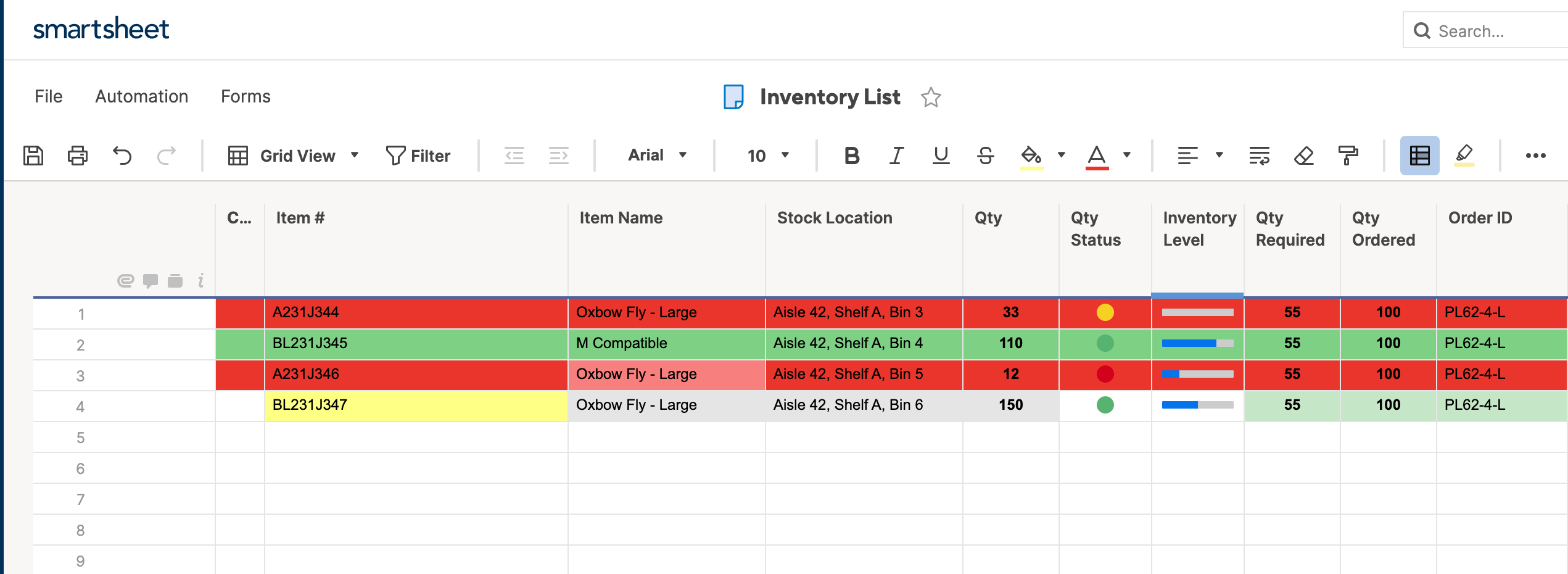
Tip: To eliminate visual redundancy, you can hide the Qty. Status column in your sheet. Simply right-click the column and click Hide column. Your sheet will retain its formatting based on that column, but it will look cleaner.

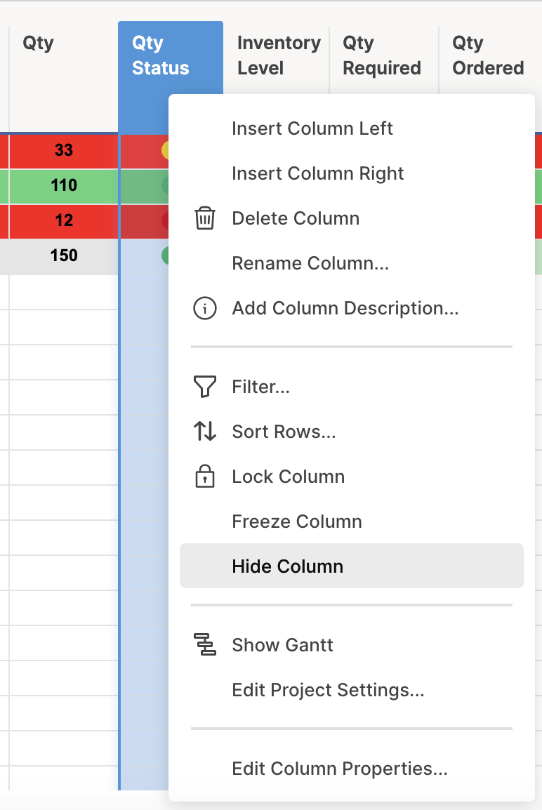
Step 4: Rule Hierarchy and Precedence

Managing rule hierarchy is quite simple in Smartsheet. The rules also interact the same way as Excel (you can apply multiple rules to a single cell, but only one will show up if there’s a conflict). However, the default precedence is a little different:

Click on the conditional formatting icon to bring up the rules.
In Smartsheet, rules higher on this list have precedence. So, the rules have descending hierarchy from the top to bottom of the list.
To change hierarchy, simply click on a rule and drag it up or down.

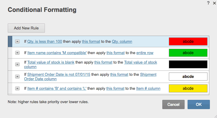
Frequently Asked Questions About Conditional Formatting

The most commonly asked questions about conditional formatting include queries about who can make changes, where to learn about using formulas, and how to copy conditional formatting rules between sheets. We’ve answered these and other frequently asked questions below:

Will conditional formatting change the values in my cells?

No. Conditional formatting only applies formatting to your cells. However, you can use conditional formatting to manipulate the values in your cells by using formulas, or by creating rules that change the value of a cell based on another cell.

Can anyone change or apply conditional formatting to the spreadsheets?

Only one person can update conditional formatting rules in Excel at a time. In Smartsheet, any collaborator with Admin permissions can create or edit conditional formatting, but editors and viewers cannot. Click the Sharing button to adjust permissions.

Does the Office 365 (cloud) version of Excel support conditional formatting?

Users can only view conditional formatting in the cloud version of Excel. To add or edit rules, download the Office 365 desktop version. Be careful of version control issues when working with Office 365.

I’m not comfortable using Excel formulas. Where can I learn more?

Here is a list of common questions for using Excel formulas with conditional formatting. For a comprehensive list of all Excel formulas, click here. For help with using formulas with conditional formatting in Smartsheet, check out these tips.

How do I add conditional formatting to a new document in Excel?

To copy conditional formatting to a new workbook or sheet, select the cells you want to copy conditional formatting from, and click the Format Paint icon. Drag your cursor over the column, rows, or document to apply the rules.

Here’s a walkthrough of this function.

Keep Your Team in Sync with Real Time Conditional Formatting in Smartsheet

Empower your people to go above and beyond with a flexible platform designed to match the needs of your team — and adapt as those needs change.

The Smartsheet platform makes it easy to plan, capture, manage, and report on work from anywhere, helping your team be more effective and get more done. Report on key metrics and get real-time visibility into work as it happens with roll-up reports, dashboards, and automated workflows built to keep your team connected and informed.

When teams have clarity into the work getting done, there’s no telling how much more they can accomplish in the same amount of time. Try Smartsheet for free, today.

Источник

Conditional formatting in excel helps format a range of cells based on the fulfillment of one or more conditions. The formatting to be applied can either be selected from the various options given in Excel or created from scratch by the user. Conditional formatting works on the rule “if this is the case, then that should be done.”

For example, if the numerical values in the range B2:B10 are less than 100, color the cells blue. The cells (of range B2:B10), which meet the specified condition (less than 100), will be colored blue.

For creating a conditional formatting rule, one should specify the following clauses:

Range clause: This represents a cell or range of cells on which conditional formatting has to be applied. It can be a named range or a selection.
Condition clause: This represents a condition (or a criterion) that needs to be satisfied by the conditional formatting rule. The condition applied can be single or multiple. But, every condition should necessarily have an “if” and “then” clause.

If the condition (in pointer “b”) is met, formatting is applied to the cell range (in pointer “a”). If not, no formatting is applied.

The purpose of applying a conditional formatting rule in excel is to analyze data based on the visualizations created. Moreover, it helps highlight the variations in data values, spot significant issues, and discover trends and patterns.

What Is Conditional Formatting In Excel?
- What Does The Conditional Formatting Feature Do In Excel?
- How To Apply Conditional Formatting In Excel?
- Examples
- Important Things To Note
- Frequently Asked Questions (FAQs)
- Recommended Articles

Conditional formatting in excel is used to format a range of cells based on the fulfillment of one or more conditions.
The option, conditional formatting is available under the Styles group in the Home Tab.
This function helps us highlight important information in our worksheet.
Conditional formatting is similar to that of cell formatting but the only difference is that the formatted cells automatically show the conditional formatting.
We can apply conditional formatting to one or more cells in the worksheet.

What Does The Conditional Formatting Feature Do In Excel?

The conditional formatting excel feature changes the appearance of a cell by changing its fill color, border, font color, and so on. With such changes, certain data cells can be distinguished from the others. This feature is available in the “styles” group of the Home tab.

A conditional formatting rule in excel can fulfill a variety of conditions. Some of these are listed as follows:

Format values greater than, less than, between, equal to
Format values above or below the average
Highlight the top or bottom 10 items
Highlight the top or bottom 10%
Highlight the duplicate or unique items
Format a date falling within a certain period
Format text containing certain words or characters
Format cells using a conditional formatting formulaConditional formatting using Formula is just changing the format of cells based on the user’s condition or criteria. The outcome will be either TRUE or FALSE if all of the formulas are logical. read more

This list is not exhaustive. One can explore more conditions or create a new conditional formatting rule in Excel.

Note: Conditional formatting is different from simple formatting in ExcelFormatting is a useful feature in Excel that allows you to change the appearance of the data in a worksheet. Formatting can be done in a variety of ways. For example, we can use the styles and format tab on the home tab to change the font of a cell or a table.read more. This is because the application of the former requires a condition to be met, while the latter is not condition-based.

How To Apply Conditional Formatting In Excel?

We can use the conditional formatting function in excel using the below steps:

Select the cells we want to format.
Go to Home Tab.
Select the Conditional Formatting option under the Styles group.
Choose the required condition from the list of options found in the Conditional Formatting drop down menu.

Let us consider some examples to understand the working of conditional formatting in Excel.

Examples

Example #1 – Apply the “Equal To” Conditional Formatting Rule To A Single Numeric Cell

The following image shows a numerical value in cell A1. We want to color the given cell (range clause) red if the value it contains is equal to 1 (condition clause).

The steps to apply conditional formatting in excel to the given cell (A1) are listed as follows:

Select cell A1. Click the “conditional formatting” drop-down from the “styles” group of the Home tab. Choose “new rule,” as shown in the following image.
The “new formatting rule” window opens, as shown in the following image. Under “select a rule type,” choose the option “use a formula to determine which cells to format.”
Click inside the box under “format values where this formula is true.” Select cell A1 on which conditional formatting should be applied. The cell reference “=$A$1” appears in this box, as shown in the following image.
Alternatively, one can type the absolute reference “=$A$1” in the box displayed within the red rectangle.
Complete the formula entered in the preceding step. The entire formula is “=$A$1=1” (exclude the beginning and ending double quotation marks).
Click “format,” shown in a red box in the following image.
The “format cells” dialog box opens, as shown in the following image. Click the “fill” tab.
Select the desired color. We have selected red. Click “Ok.”
Check the preview in the box to the right of “preview.” The formatting of cell A1 will match the preview displayed in this step.
If the preview is fine, click “Ok” in the “new formatting rule” dialog box.

Note: If the preview is not satisfactory, one can make changes by clicking the “format” button again.
Once “Ok” is clicked in the preceding step, the “new formatting rule” window closes. The output appears, as shown in the following image. Cell A1 has been colored red. This is because this cell meets the stated condition, which was, “if the value is 1, color the cell red.”
Hence, it has been proved that the value of cell A1 does equal to 1. Such validations are quite helpful when the dataset is large and one wants to know which cell contains what value.

Example #2 – Apply The “Greater Than” Conditional Formatting Rule To A Numeric Range

The succeeding image shows certain numerical values in the range A5:A19. We want to highlight the values that are greater than 30 (condition clause) in the given range (range clause).

The steps for applying the given conditional formatting rule in excel to the stated range are listed as follows:

Step 1: Select the range A5:A19 on which conditional formatting is to be applied. Subsequently, from the “conditional formatting” drop-down (in the Home tab), choose “highlight cells rules.” Next, select “greater than.”

Step 2: The “greater than” window opens, as shown in the following image. Under “format cells that are greater than,” enter 30. This is because the values greater than 30 are to be highlighted.

Select the desired color in the box to the right of “with.” We have selected “light red fill with dark red text.” Click “Ok” to proceed.

Step 3: The output is shown in the following image. Hence, the values in the range A5:A19 that are greater than 30 have been highlighted.

In total, 8 cells contain values greater than 30. Since all these cells are appearing in a different color, one can easily distinguish them from the other cells of the dataset.

Example #3 – Apply The “Duplicate Values” Conditional Formatting Rule To A Numeric Range

Working on the dataset of example #1, we want to highlight the duplicate valuesHighlight Cells Rule, which is available under Conditional Formatting under the Home menu tab, can be used to highlight duplicate values in the selected dataset, whether it is a column or row of a table.read more (condition clause) in the range A5:A19 (range clause). Use the conditional formatting technique of Excel.

The steps to highlight duplicates in the given range are listed as follows:

Step 1: From the “conditional formatting” drop-down in the Home tab, select “highlight cells rules.” Choose the option “duplicate values,” as shown in the following image.

Step 2: The “duplicate values” window appears. In the first box to the left, select “duplicate.” In the box to the right, select the required color. We have chosen “light red fill with dark red text.”

Next, click “Ok.”

Step 3: The output is shown in the following image. The duplicate values in the range A5:A19 have been highlighted in the chosen color. Hence, the duplicates can be easily distinguished from the unique values.

As the next step, one can decide whether to retain or delete the single duplicate value of the dataset. Moreover, had the dataset been much larger than the present one, identifying duplicates by mere observation would have been difficult. So, in such cases, conditional formatting would have helped the user know which cells contain duplicate values.

Example #4 – Apply “A Date Occurring” Conditional Formatting Rule To A Date Range

The following image shows some random dates of the year 2018. We want to highlight those dates in the range E4:E19 (range clause), which pertain to the current week (condition clause). Use the conditional formatting tool of Excel.

Note that this article was created in the last week of October 2018. This covers the period from October 28 to November 3 of 2018.

The steps to apply the given conditional formatting to the date range in excel are listed as follows:

Step 1: Select the range E4:E19 containing dates. From the Home tab, click the “conditional formatting” drop-down. Choose “highlight cells rules” and click the option “a date occurring.” This is shown in the following image.

Step 2: A new window titled “a date occurring” opens. Several options related to dates can be seen in the box to the left. These options are shown within a red box in the following image.

Step 3: From the box on the left, select “this week.” In the box to the right of “with,” we have chosen the color “light red fill with dark red text.” Click “Ok.”

Step 4: The output is shown in the following image. The dates falling in the current week (10/28/2018 to 11/03/2018) are highlighted. A total of four dates relate to this period.

Remember that once “this week” is selected, Excel automatically takes into account the dates of the present week. So, after selecting “this week,” had we been in the last week of December 2021, Excel would have considered this period for applying the given conditional formatting rule.

Example #5 – Apply Multiple Conditional Formatting Rules To A Single Numeric Range

The following image shows some dates and numbers in columns G and H respectively. We want to apply multiple conditional formatting rules to column H (range clause), which are listed as follows (two conditional clauses):

Highlight the numbers lying between 31 and 43 (both inclusive).
Highlight the numbers less than 0.

Use the conditional formatting feature of Excel.

Step 1: Select the range H5:H20. From the “conditional formatting” drop-down, choose “highlight cells rules.” Next, click “between.”

Note: Ignore the alignment of the label “count,” which has changed from “left” to “center” in the following image. This is due to the different versions of Excel being used to create images.

Step 2: The “between” dialog box opens. Enter the numbers 31 and 43 in the first and second boxes respectively. These are shown in a red box in the following image.

Step 3: Select the desired color for highlighting the cell values. We have chosen “yellow fill with dark yellow text.” Next, click “Ok.”

Step 4: The output is shown in the following image. The numbers of column H, which are between 31 and 43, have been highlighted.

Had there been numbers 31 and 43 in column H, they too would have been highlighted. This is because both the upper and lower limits are included in the “between” condition.

Step 5: For applying the second condition, select the formatted range H5:H20. Since we want to apply multiple conditional formatting rules to the same range, ensure that the output (H5:H20 to which formatting has been applied) of the preceding step is selected.

Next, from the “conditional formatting” drop-down, choose “highlight cells rules.” Click “less than” and the succeeding window opens.

In the box to the left, enter 0. In the box to the right, select the desired color. We have chosen “light red fill with dark red text.” Click “Ok.”

Note: It is recommended to choose different colors while applying multiple conditional formatting rules to the same excel range. This helps distinguish between the different outcomes.

Step 6: The output is shown in the following image. The negative numbers in column H have been highlighted in light red color.

Now, column H shows outcomes based on two criteria. The result of the first conditional formatting rule (between 31 and 43) is in yellow, while the result of the second one (less than 0) is in light red. In this example, the two criteria (or conditions) were not overlapping. This is the reason it is easy to compare the two outputs.

In overlapping criteria, the first condition may be to highlight numbers lying between 31 and 43. The second condition may be to highlight numbers equal to 42. In such cases, comparison between the outcomes of the two conditions may become difficult.

Note: For changing priorities of multiple conditional formatting rules, refer to the second question under the heading “frequently asked questions.” This section is given at the end of this article.

Example #6 – Apply “Data Bars,” “Color Scales,” And “Icon Sets” Formatting Methods To Multiple Numeric Ranges

In the subsequent images, the values of the “count” column (of example #4) have been pasted in three different columns titled “count1,” “count2,” and “count3.” Format the ranges L6:L21, K6:K21, and M6:M21 by using data barsData bars are a type of conditional formatting option in Excel that are used to highlight cells or data ranges in a worksheet based on certain criteria.read more, color scales, and icon setsExcel icon sets are part of the conditional formatting graphics for numerical data sets. They help design the numbers more beautifully Directional, Shapes, Indicator, and Ratings are the many types of icon sets.
read more respectively.

Show only the usage of the stated formatting methods without creating a new conditional formatting rule. There are three range clauses (three given ranges) in this example but no conditional clause.

The steps for using the stated formatting methods are listed as follows:

Step 1: Select the range L6:L21. From the “conditional formatting” drop-down, choose “data bars.” Next, select the desired color theme. We have chosen “blue data bar” from “gradient fill.”

The selection is shown in the following image. Notice that while selecting the color theme, Excel displays a preview (on the selected range) in the background.

Note: Data bars, color scales, and icon sets are the different conditional formatting techniques in excel that visually enhance the appearance of a dataset. In these techniques, the bars, shapes, color patterns, arrows, etc., are used to represent data.

Step 2: Select the range K6:K21. From the “conditional formatting” drop-down, choose “color scales.” We have selected the “green-yellow-red” color scale.

One can observe the selected theme in the background of the following image.

Step 3: Select the range M6:M21. From the “conditional formatting” drop-down, choose “icon sets.” Select the desired theme. We have selected “3 arrows (colored)” from the “directional” icon sets.

The selection is shown in the following image.

Step 4: The final output is shown in the following image. Notice how formatting has changed the appearance of the given dataset.

In all three ranges, the negative numbers have been colored differently. This helps distinguish between negative and positive numbers. For instance, -12 has been colored red (in the range K6:K21) by the color scale formatting method. With icon sets formatting, this number has been allotted a red, downward arrow (in the range M6:M21).

With the data bars formatting technique, the negative numbers (of range L6:L21) have leftward bars, while positive numbers have rightward bars. Moreover, bigger numbers have longer bars, while smaller numbers have shorter bars.

Example #7 – Apply The “Equal To” Conditional Formatting Rule By Using A VBA Code

It is possible to apply a conditional formatting rule by using a VBA code Conditional formatting is also possible in Excel VBA programming by using the ‘Format Conditions Collection’ macro/procedure. A conditional format is one that is applied only to cells that meet certain criteria, such as values above a certain threshold, positive or negative values, or values with a specific formula, and so on.read more. For instance, with the condition “A1=1,” a VBA code is written as follows:

Sub Example()
ThisWorkbook.Worksheets(1).Range(“A1”).Select
With ThisWorkbookVBA ThisWorkbook refers to the workbook on which the users currently write the code to execute all of the tasks in the current workbook. In this, it doesn’t matter which workbook is active and only requires the reference to the workbook, where the users write the code.read more.Worksheets(1).Range(“B1”)
.FormatConditions.Delete
.FormatConditions.Add Type:=xlExpression, _
Formula1:=”=A1=1″
.FormatConditions(1).Interior.ColorIndex = 46
End With
End Sub

You can download the conditional formatting template here – Conditional Formatting Excel Template.

Important Things To Note

Conditional formatting in excel formats a range of cells based on one or more conditions.
We can use this option under the Styles group in the Home Tab.
Using conditional formatting, we can apply multiple rules to a same cell.
We can also copy the conditional formatting using format painter.

Frequently Asked Questions (FAQs)

1. What is conditional formatting and when is it used in Excel?

Conditional formatting in excel helps apply a specified format to one or more cells subject to the fulfillment of a condition. Prior to applying a conditional formatting rule, the cell or cell range needs to be selected. Conditional formatting can be applied to a row, column, table, or PivotTable.

Conditional formatting eases comparisons across data values and thereby facilitates data analysis. The conditional formatting feature is used in the following situations:

a. When there is a need to distinguish some cells from the others
b. When there is a need to highlight the important information of a worksheet

Note: For details related to the working of the conditional formatting feature, refer to the examples of this article.

2. In case of multiple conditional formatting rules, which rule assumes priority in Excel? State the steps to change the precedence (priority) of the conditional formatting rules.

It is possible to apply as many conditional formatting rules to one range, as required. However, in such cases, the rule at the topmost position in the “conditional formatting rules manager” assumes the highest priority. The lower the rule in this window, the lower is its importance (priority).

The steps to change the precedence of the conditional formatting rules in excel are listed as follows:

a. Select the range on which multiple conditional formatting rules have been applied.
b. In the Home tab, click the “conditional formatting” drop-down from the “styles” group. Next, click “manage rules.”
c. The “conditional formatting rules manager” window opens. Select a rule by clicking it once.
d. Change the importance of the rules by moving them up or down with the “move up” or “move down” buttons. These buttons are in the form of upward and downward arrows displayed to the right of the “delete rule” button.
e. Select the “stop if true” checkbox, if required. When this check box is selected, Excel stops evaluation at that rule, if it evaluates to true. For instance, there are three rules and the “stop if true” checkbox is checked for the first rule. Then, either of the following outcomes can be obtained:
• If a particular cell within the selected range meets the first rule, the formatting set for this rule is applied. The remaining two rules are not evaluated for this cell.
• If a cell within the selected range does not meet the first rule, the other two rules are also evaluated and accordingly, formatting is applied.

The importance of the multiple conditional formatting rules (applied to the selected range) is changed.

3. How to copy and delete the conditional formatting rules in Excel?

The steps to copy the conditional formatting rule from one range to the other are listed as follows:

a. Select any cell of the first range to which a conditional formatting rule has been applied.
b. From the Home tab, click “format painter.” The mouse pointer changes to a paintbrush icon.
c. Click the first cell of the new range where the conditional formatting rule has to be pasted. Drag the paintbrush icon to the last cell of this range. Release the mouse when done.

The conditional formatting rule is copied to the new range.

The steps to delete (or remove) the conditional formatting rules are listed as follows:

a. Select the range from which the conditional formatting rule has to be removed.
b. From the “conditional formatting” drop-down in the Home tab, choose “clear rules.” Select an option depending on whether the formatting rule has to be cleared from the selection, worksheet, table or PivotTable.

The conditional formatting rule is cleared depending on the selections in both the preceding pointers.

Note: Alternatively, after selecting the range, one can click “manage rules” from the “conditional formatting” drop-down. The “conditional formatting rules manager” window opens. Next, remove any of the applied rules by selecting the rule and clicking “delete rule.” Note that only one rule can be selected at a time.

Need more help?

See Also

What is Conditional Formatting

How Does Conditional Formatting Work?

Cell Formatting You Can/Cannot Change

Conditional Formatting Options

Highlight Cells Rules

Greater Than…

Less Than…

Between…

Equal To…

Text that Contains…

A Date Occurring…

Duplicate Values…

Top/Bottom Rules

Top 10 Items…

Bottom 10 Items…

Top 10 %…

Bottom 10 %…

Above Average…

Below Average…

Data Bars

Color Scales

Icon Sets

Change Conditional Formatting Rule

Delete Conditional Formatting Rule

Deleting all Rules from Selection

New Rule

New Formatting Rule Dialog Box

Format all cells based on their values

Format only cells that contain

Format only top or bottom ranked values

Format only values that are above or below average

Format only unique or duplicate values

Use a formula to determine which cells to format

Common Use Cases of Conditional Formatting

Use Conditional Formatting to Highlight Alternate Rows

Use Conditional Formatting to Find & Highlight Blank Cell Rows

Use Conditional Formatting to Highlight Overdue Dates

Use Conditional Formatting to Compare Two Columns

Use Conditional Formatting to Create Search and Format Box

Highlight Rows Meeting two Separate Conditions

Checked Box Strikes Text Through

Highlight Cell when Target is Achieved

What is conditional formatting in Excel

How to use Conditional formatting in Excel

Conditional Formatting Formula Excel

Excel Conditional Formatting Based on Another Cell

Conditional Formatting Presets

Summary

What Is Conditional Formatting?

Conditional Formatting Basics

How to Apply Basic Conditional Formatting in Excel

Step 1: Apply Highlight Rules to Your Excel Spreadsheet

Step 2: Create Top/Bottom Rules

Step 3: Apply Data Bars

Step 4: Apply Color Scales

Step 5: Apply Icon Sets

Step 6: Edit and Delete Conditional Formatting Rules

How to Apply Basic Conditional Formatting in Smartsheet

Step 1: Open Your Existing Excel Spreadsheet in Smartsheet

Step 2: Apply Highlight Rules

Step 3: Apply Progress Bars (Data Bars)

Step 4: Apply Icon Sets

Step 5: Edit and Delete Conditional Formatting Rules

Advanced Conditional Formatting Functions in Excel

Step 1: Create a New Rule and Apply Stop if true Rule

Step 2: Apply Multiple Conditions to a Rule with AND Formula

Step 3: Conditional Formatting Based on Another Cell

Step 4: Data Validation and Dropdown Lists

Step 5: Rule Hierarchy and Precedence

Advanced Conditional Formatting in Smartsheet

Step 1: Add New Rule and Apply Stop If True Function

Step 2: Add Multiple Conditions to a Rule

Step 3: Conditional Formatting Based on Another Cell

Step 4: Rule Hierarchy and Precedence

Frequently Asked Questions About Conditional Formatting

Will conditional formatting change the values in my cells?

Can anyone change or apply conditional formatting to the spreadsheets?

Does the Office 365 (cloud) version of Excel support conditional formatting?