
How to check if a cell is empty or is not empty in Excel; this tutorial shows you a couple different ways to do this.
Sections:
Check if a Cell is Empty or Not — Method 1
Check if a Cell is Empty or Not — Method 2
Notes
Check if a Cell is Empty or Not — Method 1
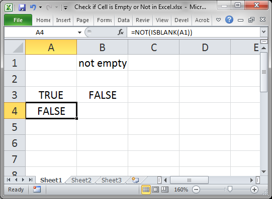
Use the ISBLANK() function.
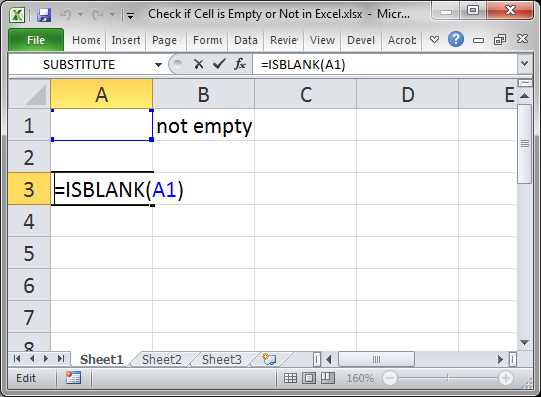
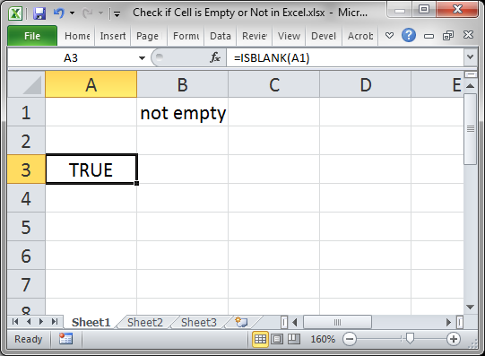
This will return TRUE if the cell is empty or FALSE if the cell is not empty.
Here, cell A1 is being checked, which is empty.
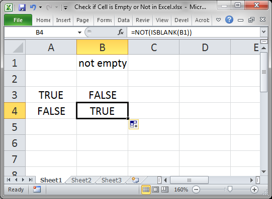
When the cell is not empty, it looks like this:
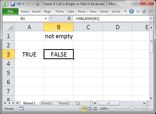
FALSE is output because cell B1 is not empty.
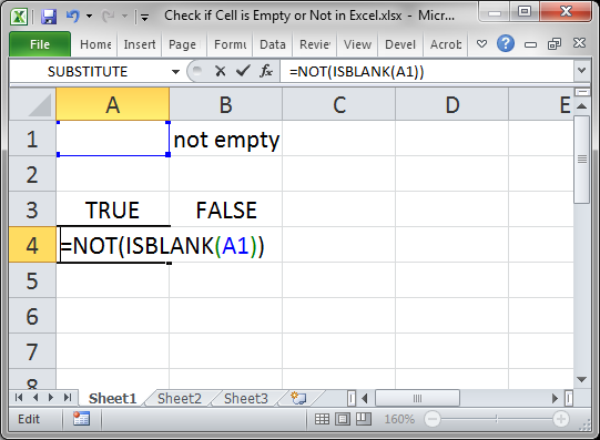
Reverse the True/False Output
Some formulas need to have TRUE or FALSE reversed in order to work correctly; to do this, use the NOT() function.
Result:
Whereas ISBLANK() output a TRUE for cell A1, the NOT() function reversed that and changed it to FALSE.
The same works for changing FALSE to TRUE.
Check if a Cell is Empty or Not — Method 2
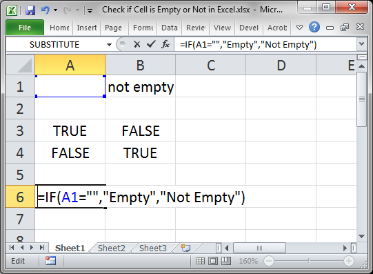
You can also use an IF statement to check if a cell is empty.
=IF(A1="","Empty","Not Empty")
Result:
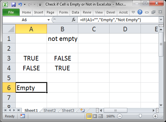
The function checks if this part is true: A1=»» which checks if A1 is equal to nothing.
When there is something in the cell, it works like this:
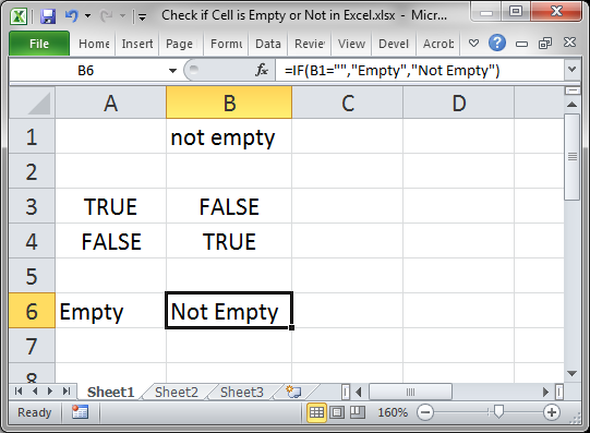
Cell B1 is not empty so we get a Not Empty result.
In this example I set the IF statement to output «Empty» or «Not Empty» but you can change it to whatever you like.
Reverse the Check
The example above checked if the cell was empty, but you can also check if the cell is not empty.
There are a few different ways to do this, but I will show you a simple and easy method here.
=IF(A1<>"","Not Empty","Empty")
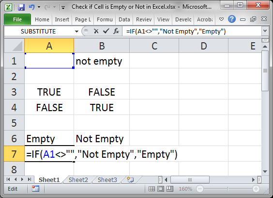
Notice the check this time is A1<>»» and that says «is cell A1 not equal to nothing.» It sounds confusing but just remember that <> is basically the reverse of =.
I also had to switch the «Empty» and «Not Empty» in order to get the correct result since we are now checking if the cell is not empty.
Result:
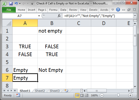
As you can see, it outputs the same result as the previous example, just like it should.
Using <> instead of = merely reverses it, making a TRUE become a FALSE and a FALSE become a TRUE, which is why «Empty» and «Not Empty» had to be reversed in order to still output the correct result.
Notes
It may seem useless to return TRUE or FALSE like in the first method, but remember that many functions in Excel, including IF(), AND(), and OR() all rely on results that are either TRUE or FALSE.
Checking for blanks and returning TRUE or FALSE is a simple concept but it can get a bit confusing in Excel, especially when you have complex formulas that rely on the result of the formulas in this tutorial. Save this tutorial and work with the attached sample file and you will have it down in no time.
Make sure to download the attached sample file to work with these examples in Excel.
Similar Content on TeachExcel
Excel VBA Check if a Cell is in a Range
Tutorial: VBA that checks if a cell is in a range, named range, or any kind of range, in Excel.
Sec…
Make Complex Formulas for Conditional Formatting in Excel
Tutorial: How to make complex formulas for conditional formatting rules in Excel. This will serve as…
Sort Data Alphabetically or Numerically in Excel 2007 and Later
Tutorial: This Excel tip shows you how to Sort Data Alphabetically and Numerically in Excel 2007. T…
Filter Data to Display the Results that Begin With Specified Text or Words in Excel — AutoFilter
Macro: This Excel macro automatically filters a set of data based on the words or text that are c…
Odd or Even Row Formulas in Excel
Tutorial: Formulas to determine if the current cell is odd or even; this allows you to perform speci…
Formula to Count Occurrences of a Word in a Cell or Range in Excel
Tutorial: Formula to count how many times a word appears in a single cell or an entire range in Exce…
Subscribe for Weekly Tutorials
BONUS: subscribe now to download our Top Tutorials Ebook!

In this article, we will learn All about Check marks and Check boxes in Excel.
What is Check Mark and Check Box?
Check box is an object which is used to create a checklist for the data. Checkbox in excel is a dependent object which shows empty or ticked depending on the condition on the cell. Whereas Checkmark is a tick symbol used in Wingdings format. While writing some information or making a checklist, where elements are marked using a small tick mark. All the elements which are considered are marked with these tick marks. Many of us like to use the same in Excel. It makes data presentable and easy to understand.
Insert Check Marks Example :
All of these might be confusing to understand. Let’s understand how to use the function using an example. Here First is by changing font style
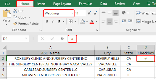
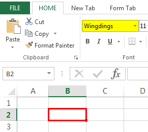
Go to Home > Select webdings in font style option and type alphabet a from the keyboard. You will see a checkmark on the selected cell.
The second method is by adding checkmark from symbols option
Go to Insert > Symbol

Symbol dialog box appears on your sheet.
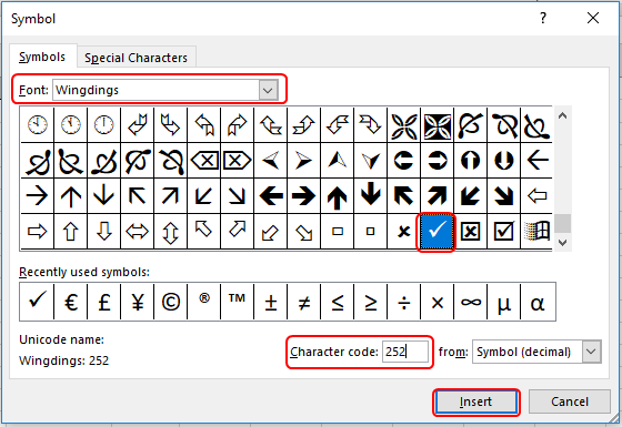
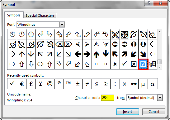
Select Wingdings in Font and type character code 252. Insert Checkmark.

As you can see check marks are added.
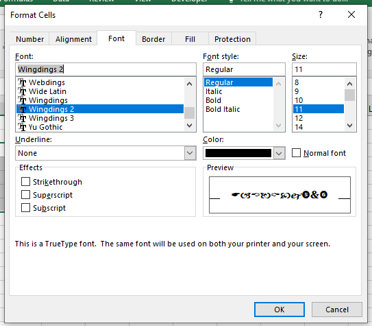
Check mark option is enabled in the format cell option. Use the Ctrl + 1 on the cell and select font option and then select wingdings 2. Wingdings 2 operate capital P as check mark in excel.
IF function excel tests the condition and returns value either it’s True or False.
Syntax of IF function:
= IF ( Logic_test , [value_if_true] , [Value_if_false] )
Logic test : operation to perform
The COUNTIF function of excel just counts the number of cells with a specific condition in a given range.
Syntax Of COUNTIF Statement
= COUNTIF ( range , condition )
Range: it is simply the range in which you want to count values.
Condition: This is where we tell Excel what to count. It can be a specific Text (should be in “”), a number, a logical operator(=,><,>=,<=,<>) and wild card operators (*,?).
We will construct a formula to do our task. In logic_test argument we will use the countif function and for the value_if_True use the Capital P.
= IF ( COUNTIF ( array , cell_value ), «P» , «» )
Let’s understand more about this function using it in an example.
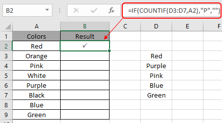
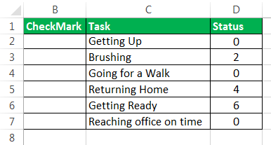
Here we have a list of colors data and and a list of colors which needed to be checked with colors data.

Here we need to use the formula to get the check mark symbol wherever required.
So we will use the formula to get the checkmark
= IF ( COUNTIF ( D3:D7 , A2 ), «P» , «» )
Explanation:
COUNTIF will return 1 if the value is found or returns 0 if not. So the COUNTIF function works fine logic test for the IF function.
The IF function returns capital P if the value is 1 or else it returns an empty string if the value is 0.
Here the arguments to the function are given as cell reference.
Copy the formula to another cell using the Ctrl + D shortcut or drag down option in excel.
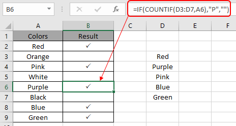
As you can see the check marks wherever required.
Insert Checkbox in Excel
To prepare the wedding checklist, we need an item list for wedding preparation, occasion, budget and checklist.
Items & Occasion:- Below are the list of Main Items and Occasions:-

Budget & %age of Items and Occasion need to spend: —Below is the list of Budget

Let’s continue with items:-
Step 1:-For every item, we have to define the sub items in which we will include each and everything. We have prepared the list for each item and occasion:-

Step 2:-
In front of list, enter the Estimated budget, Actual budget and Checklist:-
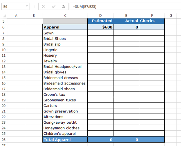
For example: -We have an Apparel list in range C6:C26.
Insert 3 columns: first for estimated budget, second for actual money spent and third for Checks
In cell D6, we will have the estimated budget which is linked to Sheet 2 where we have mentioned the estimated budget

Actual would be the sum of actual range =SUM(E7:E25)
Insert the check boxes by following below steps:-
Go to Developer tab > Controls group > Insert > Check box (form control)

After inserting the check box, right click with the mouse on check box

After inserting the check box, right click with the mouse on check box, pop up will appear

How to make a checklist?
Click on Edit text and delete the name of check box

Again, right Click on checkbox with the mouse and click on Format control from the pop-up
Format Control dialog box will appear
In Color and lines tab > Select the color for checkbox from fill color

In Color and lines tab > Select the color for checkbox

Once more, right click on the check boxes > Format Control > Control.

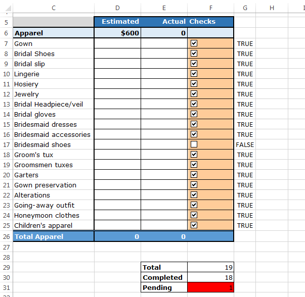
Link the cell with cell G7. When we check and uncheck the checkboxes, linked cell will change into true and false

Click on ok.

Now, copy the check box in the range and change the linked cell for every check boxes


According to the check boxes, we will return total no. of checkpoints completed and number of things that are left

Enter the formula for total nos:- =COUNTA(G7:G25)

Enter the formula for total Completed:- =COUNTIF(G7:G25,»True»)

Note: When we check the check box then the linked cell will show true and, on uncheck, the result would be false.
To return pending no. we will subtract completed numbers from total numbers

This table will be helpful to track how many items are pending in the list.
Now, we will put the Conditional Formatting on pending cells, if the number of pending cells is zero, then cell color would be highlighted in green color; in case of greater than zero, it will be highlighted in red color.
Follow the steps below:-
Select the cell of Pending numbers
Go to Home tab > Conditional Formatting >New rule

New formatting rule dialog box will appear >Use a Formula to determine which cells to format >Enter the formula in format values box> =$F$31=0
Click on Format > Format cells dialog box will appear > Fill tab > Select green color

Click on OK

For second, follow the same process
Home Tab > Conditional Formatting >New formatting rule dialog box will appear > Use a Formula to determine which cells to format > Enter the formula in format values box > =$F$31>0
Click on Format > Fill Tab > Choose Red color > Click on ok > Click on ok

Note: — If you forgot any item, then this cell will be helpful to remind you that the items are still pending in the checklist.
Now, we will do the same thing for every checklist and then our wedding checklist will get prepared.
Here are all the observational notes using the formula in Excel.
Notes :
- The function returns an error if a non-numeric value is used without a quote sign («value»).
- The function returns the check mark using the IF function with COUNTIF function.
- You can keep record of office or home budget after creating the checklist template
- You can also track the pending items basis on the checklist
Hope this article about How to use the Check mark and Check box in Excel is explanatory. Find more articles on calculating values and related Excel formulas here. If you liked our blogs, share it with your friends on Facebook. And also you can follow us on Twitter and Facebook. We would love to hear from you, do let us know how we can improve, complement or innovate our work and make it better for you. Write to us at info@exceltip.com.
Related Articles :
How to use the Shortcut To Toggle Between Absolute and Relative References in Excel : F4 shortcut to convert absolute to relative reference and same shortcut use for vice versa in Excel.
How to use Shortcut Keys for Merge and Center in Excel : Use Alt and then follow h, m and c to Merge and centre cells in Excel.
How to Select Entire Column and Row Using Keyboard Shortcuts in Excel : Use Ctrl + Space to select whole column and Shift + Space to select whole row using keyboard shortcut in Excel
Paste Special Shortcut in Mac and Windows : In windows, the keyboard shortcut for paste special is Ctrl + Alt + V. Whereas in Mac, use Ctrl + COMMAND + V key combination to open the paste special dialog in Excel.
How to Insert Row Shortcut in Excel : Use Ctrl + Shift + = to open the Insert dialog box where you can insert row, column or cells in Excel.
Popular Articles :
50 Excel Shortcuts to Increase Your Productivity : Get faster at your tasks in Excel. These shortcuts will help you increase your work efficiency in Excel.
How to use the VLOOKUP Function in Excel : This is one of the most used and popular functions of excel that is used to lookup value from different ranges and sheets.
How to use the IF Function in Excel : The IF statement in Excel checks the condition and returns a specific value if the condition is TRUE or returns another specific value if FALSE.
How to use the SUMIF Function in Excel : This is another dashboard essential function. This helps you sum up values on specific conditions.
How to use the COUNTIF Function in Excel : Count values with conditions using this amazing function. You don’t need to filter your data to count specific values. Countif function is essential to prepare your dashboard.
Excel for Microsoft 365 Excel for Microsoft 365 for Mac Excel 2021 Excel 2021 for Mac Excel 2019 Excel 2019 for Mac Excel 2016 Excel 2016 for Mac Excel 2013 Excel 2010 Excel 2007 Excel for Mac 2011 More…Less
Sometimes you need to check if a cell is blank, generally because you might not want a formula to display a result without input.

In this case we’re using IF with the ISBLANK function:
-
=IF(ISBLANK(D2),»Blank»,»Not Blank»)
Which says IF(D2 is blank, then return «Blank», otherwise return «Not Blank»). You could just as easily use your own formula for the «Not Blank» condition as well. In the next example we’re using «» instead of ISBLANK. The «» essentially means «nothing».
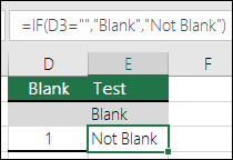
=IF(D3=»»,»Blank»,»Not Blank»)
This formula says IF(D3 is nothing, then return «Blank», otherwise «Not Blank»). Here is an example of a very common method of using «» to prevent a formula from calculating if a dependent cell is blank:
-
=IF(D3=»»,»»,YourFormula())
IF(D3 is nothing, then return nothing, otherwise calculate your formula).
Need more help?
Check marks have become a part of our task-oriented lives. If you use Excel to generate and execute lists (and you probably do), inserting an Excel check mark symbol will come in mighty handy. In this tutorial, we’ll show you how to insert a check mark in Excel.
What is a check mark?
A check mark or tick (✓) is a symbol that is universally associated with a positive response (for example, yes, completed, correct, etc.). The tick symbol in Excel is treated as text. This means that the color and size can be changed like any other text would be, and the location can be changed using the standard Copy and Paste commands.
Check marks are not the same as check boxes. A check box in Excel is an object which is placed on a worksheet. A check box that appears to be in a cell will not be deleted if that cell is deleted, because the check box is not actually a part of the cell. The location of a check box can be changed by dragging it as you would any other object.
Download your free check mark practice file!
Use this free Excel check mark file to practice along with the tutorial.
How to insert a check mark
There are multiple ways to insert a check mark in Excel. Five commonly-used methods are shown below.
Method 1: Shift P, Wingdings 2 font
A check mark is just another text character. If you can remember that SHIFT + P is that character, you can simply type an uppercase P in your desired cell, and change the font to Wingdings 2 as you would perform any regular font change. The Wingdings check mark will then be displayed in the worksheet.
 You may also care to know that SHIFT + O in the Wingdings 2 font inserts the X symbol (×).
Method 2: Insert — symbol menu
The Excel ribbon has an Insert tab, and from there a Symbol dropdown. Choose the Symbol command and you will find all the supported symbols in Excel.
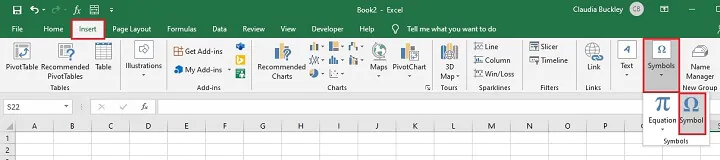 In the Symbol dialog box, choose the Wingdings font option, and scroll down to find the check mark character.
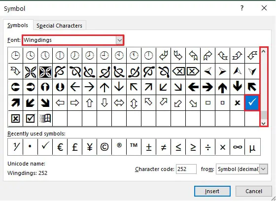 Select the check mark and click the Insert button to place the check mark in the worksheet, then click Close to close the dialog window.
You can see in the above image that Excel stores recently used symbols toward the bottom of the Symbol dialog box to save time if you need to insert them again.
Method 3: ALT 0252
If you saw the character code 252 at the bottom of the dialog box in the previous method, this might be a good reminder of an Excel check mark shortcut.
You’ll need to change the font to Wingdings, then hold the ALT button while typing in 0252. Note that the numbers should be entered from the numeric pad on the keyboard, and not from the QWERTY numbers above the letters.
 If you forgot to change the font to Wingdings before doing the ALT 0252 shortcut, you may see a character that looks like this: ü. No worries. Just change that cell to the Wingdings font and your check mark will be displayed.
Note: There is no such option on Mac devices.
Method 4: UNICHAR function
A check mark can be inserted using a function? Yes, it can. UNICHAR is a text function that returns the character represented by the Unicode argument in parentheses. Remember that each character is assigned a special code within the computer’s memory. Once you know the code for the character you want to insert, you can use UNICHAR to insert it.
=UNICHAR(10003) inserts a check mark, and UNICHAR(10004) inserts a heavy check mark.
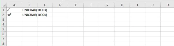 This method offers the advantage of not having to change to a special font. If you choose to use the UNICHAR function, bear in mind that the check mark has to be the only value in that cell.
UNICHAR(10007) and UNICHAR(10008) will insert the X and heavy X, respectively.
Method 5: Conditional formatting
Conditional formatting tells cells how to behave if certain conditions are met. The Conditional Formatting feature can add icons into cells based on cell values, and you can use this feature to add a check mark in Excel.
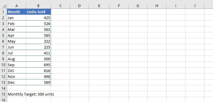
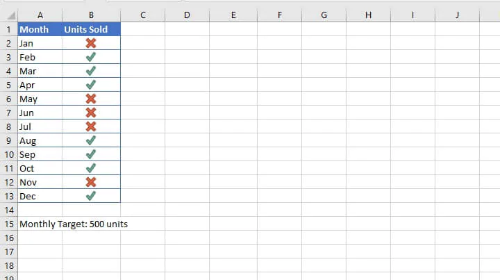
For example, download the practice file and work along while we use conditional formatting to insert a check mark next to each month where the target of 500 unit sales per month was met, and an X next to the months where the target was not met.
Download your free check mark practice file!
Use this free Excel check mark file to practice along with the tutorial.
To apply conditional formatting, follow the steps below:
- Select the range where you want to place check marks (B2 to B13).
- Go to the Home tab > click Conditional Formatting > then choose Icon Sets and select the set which includes the check mark indicator. This will be a 3-symbol icon set (a check mark, an X, and an exclamation mark).
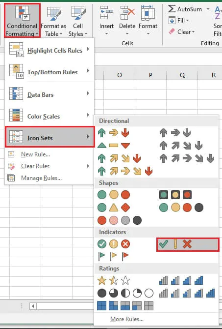 By default, Excel places a check mark for values within the 67th percentile and higher, and an X for values below the 33rd percentile. For values between the 33rd and 66th percentiles, an exclamation symbol is the default.
- Change this default rule by going to the Manage Rules button under the Conditional Formatting menu while the data range is selected. This will bring up the Conditional Formatting Rules Manager window. Click the Edit Rules command to change the conditions under which these symbols are applied.
- In the lower third of the Edit Formatting Rule window, change Percent to Number under the Type dropdown, and change the value 67 to 500. This will cause cells that are greater than or equal to 500 to have a check mark inserted.
- Just below that, change the exclamation symbol to an X from the Icon dropdown, change the >= symbol to >, the Type to Number, and the Value to 0.
- For the third symbol, click the dropdown and select No cell icon.
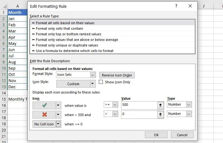
- Click OK to confirm your changes and OK to apply them and return to the worksheet.
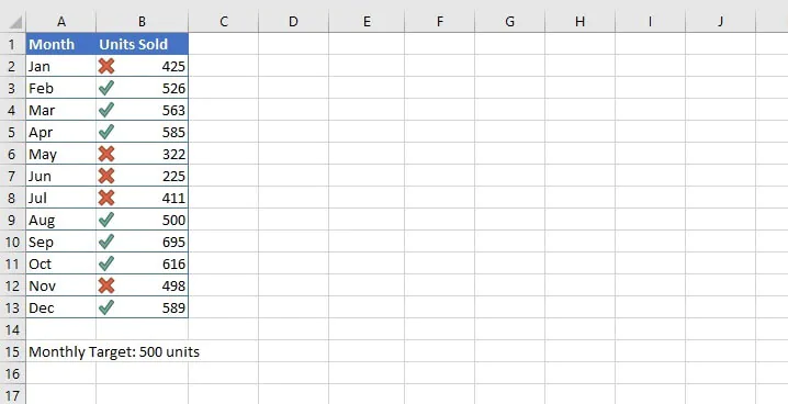 You will now be able to tell at a glance whether the monthly target was met or not.
There is also the option of displaying the symbols only, without the associated number. Do this by returning to the Conditional Formatting Rules Manager, choosing Edit Rule, and then selecting the Show Icon Only checkbox.
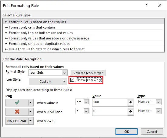 When applied, the cells will now display the icons only.
 Of course, since the check mark behaves just like a text character, you can make it bold, color it, increase the font size, change the alignment, and apply any other text formatting you like.
Learn more
Easy breezy. If you’ll be using check marks in Excel often, decide on your one or two favorite methods and practice them.
Like what you learned? Try the GoSkills range of Excel courses to see what else you can learn in Excel. You can try our Microsoft Excel — Basic and Advanced course. Or start with our free Excel in an Hour course to learn some basics in Excel.
Learn Excel for free
Start learning formulas, functions, and time-saving hacks today with this free course!
Start free course
What is Check Mark/Tick (✓) Symbol in Excel?
A check mark in Excel shows whether or not a given task is done. Remember, it is different from the checkbox. There are three simple methods to insert a checkmark in Excel. The first is just copying a tick mark and pasting it into Excel. The second option is inserting a symbol from the insert tab. The third is when we change the font to “Wingdings 2” and press the keyboard shortcut “SHIFT+P.”
For example, suppose you insert a check mark as a symbol in a cell, just as in normal text. You can also copy a check mark when we copy a cell. Moreover, you can also delete a check mark when we delete a cell. You can also format and change the font size and color like normal text.
The check marks/tick marks can be used as buttons to style our writing content. It can be illustrated in the below example.
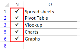
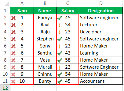
In the above example, the data in Excel is represented as different points by using the tick mark.
We can use the check mark to validation of the data in ExcelThe data validation in excel helps control the kind of input entered by a user in the worksheet.read more. Here is the below example.
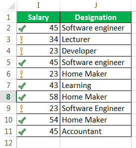
In the above example, the condition taken is salary > = 45. All the data above 45 shows the check mark; for all other data less than 45, it displays an exclamatory symbol.
Table of contents
- What is Check Mark/Tick (✓) Symbol in Excel?
- How to Make a Check Mark in Excel?
- Top 7 Ways to Put Check Mark (✓ Tick) in the Excel
- #1 – By Using Tick Symbol Option in Excel
- #2 – Using the Character Code
- #3 – Use a Keyboard Shortcut excel key to Insert Tick Mark
- #4 – Using Char Functions
- #5 – Using the Option in Conditional Formatting
- #6 – Using the ASCII Code
- #7 – From the Bullet Library
- The behavior of the Tick (✓) symbol in Excel>
- Things to Remember
- Recommended Articles
How to Make a Check Mark in Excel?
Let us follow the below steps.
- A check mark is a wonderful option in Microsoft Excel. It is present in the Insert Tab and the Symbols field.

- If we click on the Symbols, a dialogue box is displayed below.

After inserting the (✓) in the required cell, we can change the text associated with the check mark.
Users can change the user-defined text for the check mark field.
- The following process can do this.
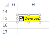
After inserting the checkbox from the Developer option, right-click on the checkbox cell and select the Edit Text option.

- Write the user-defined text in the place of the checkbox text.

The Excel tick marks are used to create checkboxes, and the checklist is used for selecting single or multiple options at a time.

Top 7 Ways to Put Check Mark (✓ Tick) in Excel
You can download this Check-Mark-Excel-Template here – Check-Mark-Excel-Template
#1 – By Using Tick Symbol Option in Excel
We know that Microsoft Office supports many symbols in Excel. The checkmark is also one of the symbols.
Go to the “Insert” tab and select the “Symbols “option.
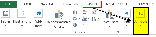
A dialogue box will appear, as shown in the below figure.
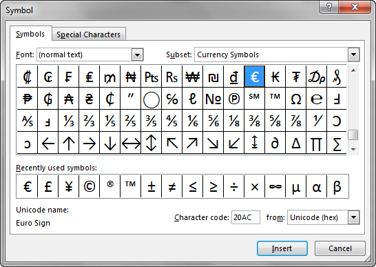
From the “Font” option, we must select the “Wingdings” font. As a result, you may find many symbols and drag the scroll bar to the end. In addition, you may find two check marks or tick marks in Excel.
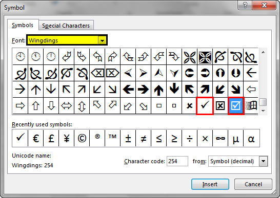
The next is the character code. The check mark’s character codes are “252 “and “254”. Now, it is time to choose the symbol we want, i.e., if the user wants only a tick mark in Excel, then “252” is the character code.

Or, if the user wants to use a check mark inside a square box, then “254” is the character code.
#2 – Using the Character Code
Step 1: We must place the cursor in the cell where we want to insert a check mark. Then, we will go to the “Home” tab and change font settings to “Wingdings.”
Step 2: We must click and hold the “ALT” key while typing the character code. Then, release the “ALT “key. As a result, the symbol we typed will be displayed in the desired cell.

The character code of the tick symbol is “0252,” and the character code of the checkmark in the square box is “0254.”
#3 – Use a Keyboard Shortcut Excel key to Insert Tick Mark
The cell or column of cells where we want to insert a checkmark needs to have the “Font” settings in the “Home” tab. The “Font” settings are that the font style should be “Wingdings 2 “or “Webdings.“
There are two shortcuts for checkmarks in “Wingdings”. There are as follows.
Shortcut 1: We must press the “Shift + P” keys to insert the tick mark symbol in Excel.

Shortcut 2: We may press the “Shift + R” keys to insert the checkmark inside a square box.

The Excel shortcutsAn Excel shortcut is a technique of performing a manual task in a quicker way.read more for check marks in the “Webdings” font style. We should follow the above rule of font settings like the “Wingdings.”
Keyboard shortcut: “a” is the shortcut for a checkmark in this font style.
#4 – Using Char Functions
Microsoft Excel supports many functions in addition to formulas and shortcuts.
Char() is the function in ExcelThe character function in Excel, also known as the char function, identifies the character based on the number or integer accepted by the computer language. For example, the number for character «A» is 65, so if we use =char(65), we get A.read more that can display the characters, special symbols, etc., whenever necessary.
Example: char(252)
=IF(C2=0, CHAR(252),"")

#5 – Using the Option in Conditional Formatting
For this, select the“ Home” tab, then go to conditional formattingConditional formatting is a technique in Excel that allows us to format cells in a worksheet based on certain conditions. It can be found in the styles section of the Home tab.read more, and in the drop-down, select the “Icon Sets” option.
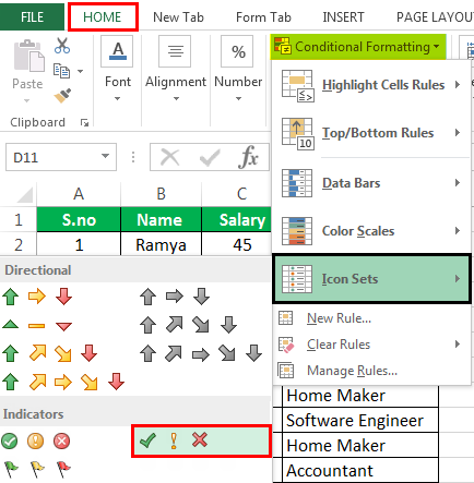
Then you can see the check marks in your data according to the conditions.
#6 – Using the ASCII Code
The ASCII code of the check mark is obtained using the ASCII character. For example, the ASCII character of the checkmark is Ü, and the ASCII code of the checkmark is 252.
#7 – From the Bullet Library
We can find the tick mark symbol in Excel’s “Bullet Library.”
That can be used as a bullet option.
Go to the Home tab -> Bullet Library -> select Tick Mark.
The behavior of the Tick (✓) symbol in Excel>
- Like the normal text and other numeric characters, the symbols behave similarly.
- We can make the check mark “Bold “or “Italic “by applying the styles.
- We can fill the cell color with the required color.
- We can change the tick mark color to another by changing it from the home tab.
- Like the check mark in Excel, we can use another option manually and check that option whenever necessary. That is called a checkbox.
Things to Remember
- Unlike Radio buttons in ExcelIn Excel, radio buttons or options buttons record a user’s input. They can be found in the developer’s tab’s insert section. read more, we can select this check mark in multiple numbers.
- We can use this check mark to fill out any survey or application forms to choose the criteria.
- The checkmark is also used to determine the compulsory options while reading the privacy policy.
Recommended Articles
This article is a guide to Check Mark in Excel. We discuss the methods to insert check mark/tick mark in Excel, examples, and a downloadable template. You may learn more about Excel from the following articles: –
- Match Data in Excel
- Format in Excel
- Excel Add Months to Date
- How to Remove Watermark in Excel Sheet?