What is a cell style in excel

To apply several formats in one step, and to make sure that cells have consistent formatting, you can use a cell style. A cell style is a defined set of formatting characteristics, such as fonts and font sizes, number formats, cell borders, and cell shading. To prevent anyone from making changes to specific cells, you can also use a cell style that locks cells.

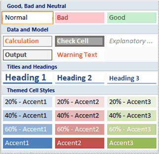
Microsoft Office Excel has several built-in cell styles that you can apply or modify. You can also modify or duplicate a cell style to create your own, custom cell style.

Important: Cell styles are based on the document theme that is applied to the whole workbook. When you switch to another document theme, the cell styles are updated to match the new document theme.

1. Select the cells that you want to format. For more information, see Select cells, ranges, rows, or columns on a worksheet.

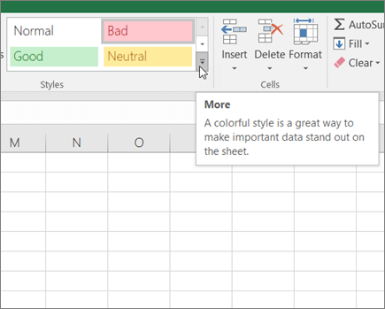
2. On the Home tab, in the Styles group, click the More dropdown arrow in the style gallery, and select the cell style that you want to apply.

   

1. On the Home tab, in the Styles group, click the More dropdown arrow in the style gallery, and at the bottom of the gallery, click New Cell Style.

2. In the Style name box, type an appropriate name for the new cell style.

3. Click Format.

4. On the various tabs in the Format Cells dialog box, select the formatting that you want, and then click OK.

5. Back in the Style dialog box, under Style Includes (By Example), clear the check boxes for any formatting that you do not want to include in the cell style.

6. Click OK.

1. On the Home tab, in the Styles group, click the More dropdown arrow in the style gallery.

   

2. Do one of the following:

   • To modify an existing cell style, right-click that cell style, and then click Modify.

   • To create a duplicate of an existing cell style, right-click that cell style, and then click Duplicate.

3. In the Style name box, type an appropriate name for the new cell style.

   Note: A duplicate cell style and a renamed cell style are added to the list of custom cell styles. If you do not rename a built-in cell style, the built-in cell style will be updated with any changes that you make.

4. To modify the cell style, click Format.

5. On the various tabs in the Format Cells dialog box, select the formatting that you want, and then click OK.

6. In the Style dialog box, under Style Includes, select or clear the check boxes for any formatting that you do or do not want to include in the cell style.

You can remove a cell style from data in selected cells without deleting the cell style.

1. Select the cells that are formatted with the cell style that you want to remove. For more information, see Select cells, ranges, rows, or columns on a worksheet.

2. On the Home tab, in the Styles group, click the More dropdown arrow in the style gallery.

   

3. Under Good, Bad, and Neutral, click Normal.

You can delete a predefined or custom cell style to remove it from the list of available cell styles. When you delete a cell style, it is also removed from all cells that are formatted with it.

1. On the Home tab, in the Styles group, click the More dropdown arrow in the style gallery.

   

2. To delete a predefined or custom cell style and remove it from all cells that are formatted with it, right-click the cell style, and then click Delete.

   Note: You cannot delete the Normal cell style.

1. Select the cells that you want to format. For more information, see Select cells, ranges, rows, or columns on a worksheet.

2. On the Home tab, in the Styles group, click Cell Styles.

   

   Tip: If you do not see the Cell Styles button, click Styles, and then click the More button next to the cell styles box.

3. Click the cell style that you want to apply.

1. On the Home tab, in the Styles group, click Cell Styles.

   

   Tip: If you do not see the Cell Styles button, click Styles, and then click the More button next to the cell styles box.

2. Click New Cell Style.

3. In the Style name box, type an appropriate name for the new cell style.

4. Click Format.

5. On the various tabs in the Format Cells dialog box, select the formatting that you want, and then click OK.

6. In the Style dialog box, under Style Includes (By Example), clear the check boxes for any formatting that you do not want to include in the cell style.

1. On the Home tab, in the Styles group, click Cell Styles.

   

   Tip: If you do not see the Cell Styles button, click Styles, and then click the More button next to the cell styles box.

2. Do one of the following:

   • To modify an existing cell style, right-click that cell style, and then click Modify.

   • To create a duplicate of an existing cell style, right-click that cell style, and then click Duplicate.

3. In the Style name box, type an appropriate name for the new cell style.

   Note: A duplicate cell style and a renamed cell style are added to the list of custom cell styles. If you do not rename a built-in cell style, the built-in cell style will be updated with any changes that you make.

4. To modify the cell style, click Format.

5. On the various tabs in the Format Cells dialog box, select the formatting that you want, and then click OK.

6. In the Style dialog box, under Style Includes, select or clear the check boxes for any formatting that you do or do not want to include in the cell style.

You can remove a cell style from data in selected cells without deleting the cell style.

1. Select the cells that are formatted with the cell style that you want to remove. For more information, see Select cells, ranges, rows, or columns on a worksheet.

2. On the Home tab, in the Styles group, click Cell Styles.

   

   Tip: If you do not see the Cell Styles button, click Styles, and then click the More button next to the cell styles box.

3. Under Good, Bad, and Neutral, click Normal.

You can delete a predefined or custom cell style to remove it from the list of available cell styles. When you delete a cell style, it is also removed from all cells that are formatted with it.

1. On the Home tab, in the Styles group, click Cell Styles.

   

   Tip: If you do not see the Cell Styles button, click Styles, and then click the More button next to the cell styles box.

2. To delete a predefined or custom cell style and remove it from all cells that are formatted with it, right-click the cell style, and then click Delete.

   Note: You cannot delete the Normal cell style.

Need more help?

You can always ask an expert in the Excel Tech Community or get support in the Answers community.

A cell style is a defined set of formatting characteristics, such as fonts and font sizes, number formats, cell borders, and cell shading.Microsoft Office Excel has several built-in cell styles that you can apply or modify. You can also modify or duplicate a cell style to create your own, custom cell style.

Finally, the Styles group lets users to apply criteria based formatting to cell in Excel. Also, we might use the inbuilt templates; of Format as Table & Cell Styles buttons for Table and Cells. To emphasize, these various templates is based on color with different shades, styles in Microsoft Excel.

Where is cell style in Mac Excel?

Apply a cell style
Select the cells that you want to format. On the Home tab, click Cell Styles, and then select the style that you want.

What is a cell style?

A cell style is a defined set of formatting characteristics, such as fonts and font sizes, number formats, cell borders, and cell shading. To prevent anyone from making changes to specific cells, you can also use a cell style that locks cells.

What is Comma style format in Excel?

Comma style is a formatting style used in visualizing numbers with commas when the values is over 1000, such as if we use this style on data with value 100000 then the result displayed will be as (100,000), this formatting style can be accessed from the home tab in the number section and click on the 1000 (,) separator

How do I count cell styles in Excel?

#1 Count Colored Cells Using Filter and SUBTOTAL

1. In any cell below the data set, use the following formula: =SUBTOTAL(102,E1:E20)
2. Select the headers.
3. Go to Data –> Sort and Filter –> Filter. This will apply a filter to all the headers.
4. Click on any of the filter drop-downs.
5. Go to ‘Filter by Color’ and select the color.

What is Accent 6 Excel?

Orange color (accent 6, darker 50%)
– Select your particular cells assume that, A1:H16. – Select background color as Red with black border and Click ok. – Select background color as Orange and Click ok.

How do I pin cell styles in Excel?

1. Click the Cell Styles button. Right-click the style you want to duplicate, and then click Duplicate.
2. In the Style dialog box, modify the name of your style and select the elements to include in the style.
3. Click the Format button.
4. Use the controls in the Format Cells dialog box to define your style.
5. Click OK.

What is Accent 1 Excel?

To apply a cell style:
Select the cell(s) you want to modify. Click the Cell Styles command on the Home tab, then choose the desired style from the drop-down menu. In our example, we’ll choose Accent 1. The selected cell style will appear.

Which elements are included in cell styles?

In Microsoft Excel, cell style refers to the various appearances that can be applied to a cell, or the text contained within it. Some of the style elements include background color of the cell, border style for the cell, font type, font size, bold, italics, underline, strikethrough, and others.

What is 3D formula in Excel?

A 3D formula is a formula that refers to the same cell (or range of cells) on multiple worksheets. The 3D formula “=SUM(Sheet1:Sheet4! A2)” can be used to add up the numbers in cell “A2” on 4 different worksheets.

What is an absolute cell reference?

In contrast, the definition of absolute cell reference is one that does not change when it’s moved, copied or filled. This way, the reference points back to the same cell, no matter where it appears in the workbook. It’s indicated by a dollar sign in the column or row coordinate.

How do you put a comma after 3 digits in Excel?

Number

1. Decimal places – The number of decimal places can be from 0 to 30 and this can be changed by either typing directly into the box or using the spinner button.
2. Use 1000 separator – The 1000 separator will insert a comma every 3 digits, i.e. hundred, thousand etc.

Where are borders on Excel?

Select a cell or a range of cells to which you want to add borders. On the Home tab, in the Font group, click the down arrow next to the Borders button, and you will see a list of the most popular border types. Click the border you want to apply, and it will be immediately added to the selected cells.

Can you Countif by color?

The short answer is that COUNTIF cannot be used to check for background color or any formatting; it can only test for values. If you only need to figure out the number of purple cells once or twice, you can use Excel’s Find and Replace feature to figure it out.

How do I add Coloured cells in Excel?

Select a range or ranges where you want to count colored cells or/and sum by color if you have numerical data. Press and hold Ctrl, select one cell with the needed color, and then release the Ctrl key. Press Alt+F8 to open the list of macros in your workbook. Select the SumCountByConditionalFormat macro and click Run.

Where is Paste Special in Excel?

Using the Ribbon: Go to Home –> Clipboard –> Paste –> Paste Special. This will open the Excel Paste Special Dialogue box. Using Keyboard Shortcut: Use the Excel Paste Special Shortcut – Alt + E + S + V. Using Right-click Menu: Right Click in the cell where you want to paste, and then select paste special.

Where is Green Accent 6 Excel?

Select cells from B3 to B5. From the drop-down menu select the color Green, Accent 6.

How do you AutoFill in Excel?

Click and hold the left mouse button, and drag the plus sign over the cells you want to fill. And the series is filled in for you automatically using the AutoFill feature. Or, say you have information in Excel that isn’t formatted the way you need it to be, such as this list of names.

How do you import cell styles?

Copy cell styles from another workbook

1. Open the workbook that contains the cell styles that you want to copy.
2. Open the workbook that you want to copy the styles into.
3. On the Home tab, in the Styles group, click the More button.
4. Click Merge Styles.

How do you copy cell styles?

Copy cell formatting

1. Select the cell with the formatting you want to copy.
2. Select Home > Format Painter.
3. Drag to select the cell or range you want to apply the formatting to.
4. Release the mouse button and the formatting should now be applied.

Home > Microsoft Excel > How to Use Cell Styles in Excel: A Step-by-Step Guide

(Note: This guide on how to use cell styles in Excel is suitable for all Excel versions including Office 365)

Consider an Excel sheet that has data of different types and formats. The data might be downloaded, inserted, or circulated between users one after the other. In those cases, each data might have different formatting depending on the user settings. This will make the data unpleasant to look at and hinders its readability.

You would then want to modify and organize the data in a well-formatted and orderly fashion. You can select each cell or cell range and modify the look and format of the cell manually. However, this task can be a little daunting and time-consuming. 

Here, using the Cell Styles option in Excel you can easily modify the formatting and profile of the cell and its contents with the click of a button.

In this article, I will show you how to apply built-in styles, create custom styles, and remove the cell styles in Excel when not necessary.

You’ll Learn:

• What Are Cell Styles in Excel?
• How to Use Cell Styles in Excel?
  • Apply Built-In Cells Styles
  • Create a Custom Cell Style
  • Customize an Existing Style
  • Duplicate a Cell Style
  • Remove the Cell Style
  • Delete Cell Styles

Watch this video on How to Use Cell Styles in Excel in an easy way

Related Reads:

The 7 Golden Rules of Excel Spreadsheet Design

How to Create Excel Drop Down List With Color?

How to Graph a Function in Excel? 2 Easy Ways

What Are Cell Styles in Excel?

Cell Style refers to formatting and features that you can customize in a cell. The features that can be modified using cell styles include the font style, font color, color fill, format type, cell borders, cell color, and much more. 

Cell Styles have similar characteristics to Conditional Formatting. In Conditional Formatting, the format of the cells is changed when specific conditions or criteria are met. Whereas, Cell Styles are static i.e. you can change the cell styles whenever you want based on your needs.

The cell styles option will be very useful when you have to change the style formatting of a group of cells altogether instead of changing them one by one. You can create a particular cell style by including all the cell format aspects like font color, size, font style, fill, borders, etc., and then use them whenever needed. 

Using the built-in or custom-created cell styles will make all the cells look more consistent and give a professional finish to the data, thereby making it easier to read.

There are a variety of options available when it comes to cell styling in Excel. You can do the following: 

• Apply the Built-In Cell Styles in Excel
• Create a Custom Cell Style
• Copy and Duplicate an Existing Cell Style
• Modify an Existing Cell Style
• Remove the Cell Style from the Cells
• Delete a Cell Style

In this guide, I will explain how to use Cell Styles with an example. 

Consider an example, where you have a consolidated list of sales made by an automobile company in 11 years. 

When you enter the data onto an Excel sheet, the formatting will be different for numbers and texts. Also, there is no distinction or highlights to show the differentiation of data. You can now use the Cell Styles to format the cells and their contents.

How to Use Cell Styles in Excel?

We have recently understood what cell styles are and how you can customize cells using them. Let us now see how to use cell styles effectively to get the best profile overall. 

Apply Built-In Cells Styles

First, let us see how to apply the built-in cell styles in Excel. This is the first and foremost step when it comes to formatting a cell. After this, we can see how to create custom styles and change them.

• First, select a cell or a group of cells. In this case, let us apply the cell style to the headers i.e. the vehicle types from rows A5 to F5.

• Now, navigate to Home. Under the Styles section, click on the dropdown from Cell Styles. When you click the dropdown, you can see a variety of cell styles with different fill colors, border colors, and fonts. Since we are formatting the heading, let us select the Heading 2 style.

• Once you select your desired cell style, the style with the formatting will be applied to the selected cells.

Create a Custom Cell Style

Even though there are a variety of cell styles to choose from, there might be some instances where you might not be satisfied with the available options. In such instances, you can create your custom style with the necessary options to suit your purpose.

• To create a custom cell style, first, select a cell or range of cells. 

• Go-to Home. From the dropdown from Cell Styles, click on New Cell Style.

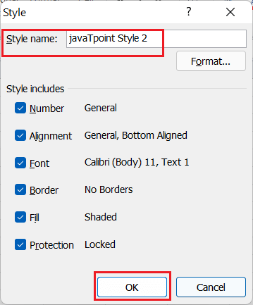
• This opens up a Style dialog box. Under Styles Includes (By example), you can see the different format options the cell is formatted for. You can choose to uncheck the checkboxes if you don’t want to include that particular aspect in the cells. 

Now, let’s get to formatting the styles. 

• From the Style Name textbox, you can set the name of the custom style.

• To change the other aspects of the cell, click on Format. This opens up the Format dialog box. Under the tabs provided, you can change the formatting type, font, border, color, and alignment of the cells. Additionally, you can also choose to lock and protect the cells to prevent them from being edited.

• After making all the necessary changes, click OK.

• This adds the custom style in the Cell Styles dropdown. 

• If you want to change the cell style, you can do it with a click. Select the cells you want to format, then select the custom format you created from the Cell Styles dropdown. 

Suggested Reads:

How to Create an Excel Slicer? 2 Easy Ways

How to Convert Excel to Word? 2 Easy Methods

How to Make a Pareto Chart Excel Dashboard? 4 Easy Steps

Customize an Existing Style

When working on cell styles, you might sometimes feel the existing styles to be a little inadequate. You also don’t want to create a cell style from scratch. In such cases, you can just tweak and modify the existing styles a little to create your style. 

• To modify an existing style, click on the dropdown from Cell Styles.

• Right-click on the style you want to customize and click on Modify. 

• When you click on Modify, the Style dialog box opens. 

• In the same way, check the checkboxes for the formatting features you want to include in the cell style. For additional settings related to font style, color, border, alignment, and protection, click on Format. 

• This opens the Format Cells dialog box. Select and customize all the necessary options and click on OK.

• Now, if you click on the dropdown from Cell Styles, you can see the default built-in font modified based on your input options.

Note: To change the modified built-in style to its default state, right-click on the style and click on Delete.

Duplicate a Cell Style

It is always a good practice to copy a cell style and then modify them instead of overriding the existing cell style. In such cases, you can duplicate a built-in or custom cell style and modify them.

• To duplicate a cell style, go to Home and click on the dropdown from Cell Styles. This shows you a list of built-in and custom cell styles.

• Now, right-click on the style you want to duplicate and select Duplicate.

• This in turn opens the Styles dialog box. Select the format features you want to include using the Format option. 

• Click OK.

• Now, the duplicated font gets saved under the Custom section of the Cell Styles dropdown. You can now use the style whenever needed. 

Remove the Cell Style

In case you are not satisfied with the cell style, you can either change the cell style or remove them. 

• To remove the cell style, first, select the cells with a particular cell style. 

• Navigate to Home. Click on the dropdown from Cell Styles. Select Normal.

• This removes the cell styles for the formatted cells and the cells are reset to the default cell styling.

Delete Cell Styles

Often, deleting and removing a particular thing might be synonymous. Here, deleting a cell style and removing a cell style are two different things. When removing, you remove the formatting of the cells and change them back to their default state. When you delete a Cell Style, you delete the particular cell style from the repository. 

You can delete a cell style if you are not satisfied with the style formatting or if you won’t need them anymore. 

• To delete a cell style, go to Home. Click on the dropdown from the Cell Styles. 

• Right-click on the cell style you want to delete and click on Delete.

• This deletes the particular cell style from the cell style repository.

Note: When you delete a cell style, all the cells which have the particular cell style will be deleted and the cells will be set to Normal (default) cell style.

Also Read:

How to Create a Funnel Chart in Excel? 2 Useful Ways

How to Insert a Hyperlink in Excel? 3 Easy Ways

How to Save Excel Chart as Image? 4 Simple Ways

Frequently Asked  Questions

Closing Thoughts

Cell Styles help combine a lot of attributes and aspects of a cell into a single click. They are an essential factor in Excel that greatly help in improving the readability and presentability of the data. 

In this article, we saw how to apply a cell style, modify, duplicate a cell style, create a custom cell style, remove a cell style, and even delete them. Depending on your needs, you can choose to use any option that suits your purpose the best. 

Please visit our free resources center for more high-quality Excel guides. 

Ready to take the next step and hone your skills in Excel?

Simon Sez IT has been teaching Excel for over ten years. For a low, monthly fee you can get access to 140+ IT training courses. Click here for advanced Excel courses with in-depth training modules.

How to Format Excel Spreadsheets Using Cell Styles

Create professional-looking work

Updated on February 23, 2020

Formatting your Excel spreadsheets gives them a more polished look, and can also make it easier to read and interpret the data, and thus better suited for meetings and presentations. Excel has a collection of pre-set formatting styles to add color to your worksheet that can take it to the next level.

These instructions apply to Excel for Microsoft 365 and Excel 2019, 2016, 2013, and 2010.

What Is a Cell Style?

A cell style in Excel is a combination of formatting options, including font sizes and color, number formats, cell borders, and shading that you can name and save as part of the worksheet.

Apply a Cell Style

Excel has many built-in cell styles that you can apply as is to a worksheet or modify as desired. These built-in styles can also serve as the basis for custom cell styles you can save and share between workbooks.

1. Select the range of cells you want to format.

2. On the Home tab of the ribbon, select the Cell Styles button in the Styles section, to open the gallery of available styles.

3. Select the desired cell style to apply it.

Customize Cell Styles

One advantage of using styles is that if you modify any cell style after applying it in a worksheet, all cells using that style automatically update to reflect the changes.

Further, you can incorporate Excel’s lock cells feature into cell styles to prevent unauthorized changes to specific cells, worksheets, or workbooks.

You can also customize cell styles either from scratch or using a built-in style as a starting point.

1. Select a worksheet cell.

2. Apply all desired formatting options to this cell.

3. On the Home tab of the ribbon, select the Cell Styles button in the Styles section, to open the gallery of available styles.

4. Select New cell styles at the bottom of the gallery.

5. Type a name for the new style in the Style name box.

6. Select the Format button in the Style dialog box to open the Format Cells dialog box.

7. Select a tab in the dialog box to view the available options.

8. Apply all desired changes.

9. Select OK to return to the Style dialog box.

10. Underneath the name is a list of the formatting options that you selected. Clear the checkboxes for any unwanted formatting.

11. Select OK to close the dialog box and return to the worksheet.

The new style’s name will now appear at the top of the Cell Styles Gallery under the Custom heading. To apply your style to cells in a worksheet, follow the steps above for using a built-in style.

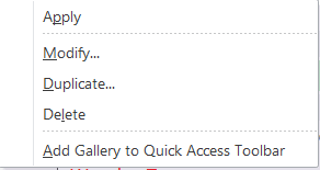
To edit cell formatting, launch the Cell Styles Gallery and right-click on a cell style and choose Modify > Format. The right-click menu also includes a Duplicate option.

Copy a Cell Style to Another Workbook

When you create a custom cell style in a workbook, it’s not available across Excel. You can easily copy custom styles to other workbooks, though.

1. Open the first workbook containing the custom style you want to copy.

2. Open the second workbook.

3. In the second workbook, select Cell Styles on the ribbon to open the Cell Styles gallery.

4. Select Merge Styles at the bottom of the gallery to open the Merge Styles dialog box.

5. Select the name of the first workbook and choose OK to close the dialog box.

An alert box will pop up asking if you want to merge styles with the same name. Unless you have custom styles with the same name but different formatting options in both workbooks, click the Yes button to complete the transfer into the destination workbook.

Remove Cell Style Formatting

Finally, you can remove any formatting you apply to a cell without deleting the data or the saved cell style. You can also delete a cell style if you no longer want to use it.

1. Select the cells that are using the cell style that you want to remove.

2. On the Home tab of the ribbon, select the Cell Styles button in the Styles section, to open the gallery of available styles.

3. In the Good, Bad, and Neutral section near the top of the gallery, select Normal to remove all applied formatting.

The above steps can also be used to remove formatting that has been applied manually to worksheet cells.

Delete a Style

You can delete any built-in and custom cell styles from the Cell Styles gallery except for Normal, which is the default. When you delete a style, any cell that was using it will lose all associated formatting.

1. On the Home tab of the ribbon, select the Cell Styles button in the Styles section, to open the gallery of available styles.

2. Right-click on a cell style to open the context menu and choose Delete. The cell style is immediately removed from the gallery.

Thanks for letting us know!

Get the Latest Tech News Delivered Every Day

Subscribe

MS Excel or Microsoft Excel is powerful spreadsheet software with a distinct range of built-in features and functions. It can handle vast amounts of data and supports various formatting options for data recorded within the spreadsheets. Excel has different formatting options to format our worksheets quickly, from simply copying the formatting from other cells to predefined conditional formatting. Apart from this, Cell style is another wonderful feature for formatting Excel cells within the sheets.

This article discusses the brief introduction of Cell Styles in Excel and the step-by-step tutorial to apply predefined Cell Styles and create custom Cell Styles in Excel.

What is Cell Style in Excel?

A cell style refers to a combination of many formats or attributes that we can apply within the Excel cells. Although we can apply each combined formatting separately, it will take more time. Instead of using various formatting separately, we better apply a single style to simultaneously implement a collection of formats. A cell style is a quick way to change the appearance of the sheet efficiently.

A cell style can combine preferences for the six attributes described below:

• Fonts (type, color, and size)
• Alignment (vertical and horizontal)
• Number Format
• Pattern
• Borders
• Protection (locked & hidden)

We can combine the above formats into a single cell style. For example, we can create a style that includes settings for a specific font color, a cell background color, and italic font style, a cell border, and a number format. Whenever we need to use such a combination of formatting, we can quickly apply them all by simply selecting the style we created instead of applying each format one by one. It helps us apply multiple formats at once with a few clicks quickly and adds consistency to the overall look of the worksheet.

How is a cell style helpful in Excel?

Although cell styles in Excel are not as powerful as Word, they are helpful and save time to apply complex formatting within the sheet quickly. For example, consider that we have entered some data to around forty to fifty cells with the font size of 12 pt. But, later, we realized that we needed to use the font size of 16 pt. in all those cells instead of 12 pt. In such a case, we can edit the cell style and put the font of 16 pt., rather than editing the font size of each corresponding cell. All the cells with that specific style will automatically change to the font size of 16 pt.

Likewise, we can also modify the other attributes (such as font type, color, size, number format, borders, vertical and alignment, etc.) through a cell style.

How to use Cell Styles in Excel?

Excel typically offers two efficient options to use cell styles on a selected cell or a range of multiple cells. We can either use any of the existing cell styles installed within Excel or create our custom style manually by choosing specific fonts, colors, shades, etc.

An existing cell style is the combination of formatting options already created and ready for us to use to desired cell or range of cells. Excel has a wide range of existing cell styles divided into different types: Normal, Bad, Good, and Neutral. Furthermore, the styles are divided based on different data types as well. For example, Data and Model. The existing cell styles cover almost everything from titles and headings to color in different elements and accents to currency and number formats.

We need to perform the following steps to use or apply existing/ predefined cell styles in Excel:

• First, we need to select the specific cell or a range of multiple cells to which we wish to apply the style.
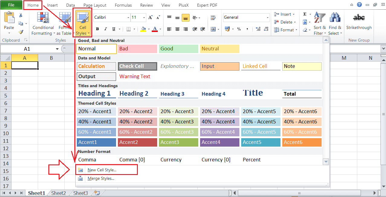
• After selecting the desired cells, we need to go to the Home tab and click on the drop-down icon associated with the ‘Cell Styles‘ option under the Styles
  
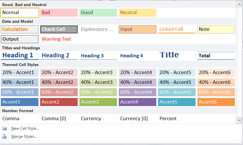
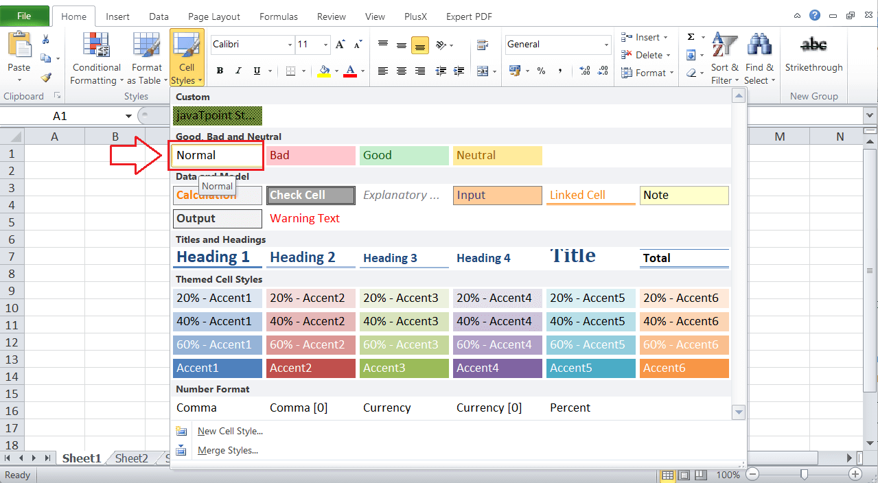
• Clicking on the Cell Styles drop-down icon will launch a pop-up window, as shown below:
  
  In the above image, these are the existing cell styles in Excel. We can click on the desired cell style, and the same will be instantly applied to the selected cell or range within the active sheet. Apart from this, we can also check the live preview of any particular style by moving the mouse pointer over it. As soon as our pointer hovers on a specific style, Excel displays the corresponding style temporarily on the selected cell or a range.

In this way, we can apply existing or default cell styles in Excel.

How to create a Cell Style in Excel?

Although Excel has several default cell styles, we may sometimes need our specific style to use in any particular workbook. We can create a custom cell style with desired settings for each corresponding format within the style. Whenever we want to use our custom style, we can select it and reuse it like the Excel default cell styles.

We need to perform the following steps to create a custom cell style in Excel:

• First, we need to select a cell or a range of cells.
• Next, we need to go to the Home > Cell Styles and click on the ‘New Cell Style‘ option, as shown below:
  
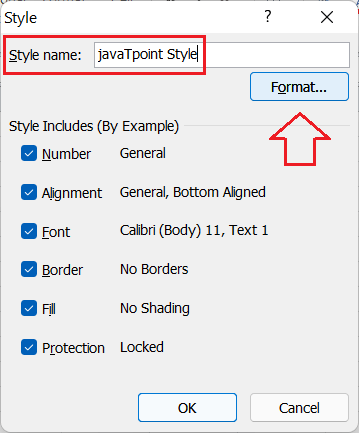
• In the next window, Excel displays the existing preferences of applied style. We can enter a name for our style at the top of the window next to the ‘Style name‘. After entering the name for our custom style, we need to click on the ‘Format‘ button to specify formatting preferences.
  
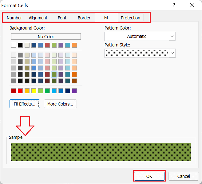
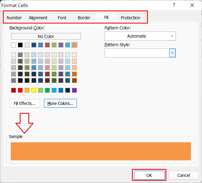
• After clicking the Format button from the Style window, we will see the Format Cells dialogue box. In the Format Cells dialogue box, we need to go through all the tabs and choose the desired preferences like the number, font, border, etc.
  
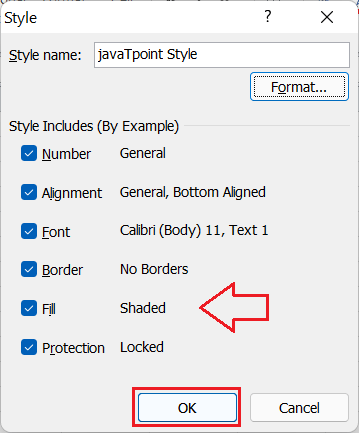
  We selected the green background in the above image with automatic pattern color and dotted pattern style.
• After choosing the desired preferences through different tabs, we need to click the OK It will again move us back to the Style window, as shown below:
  
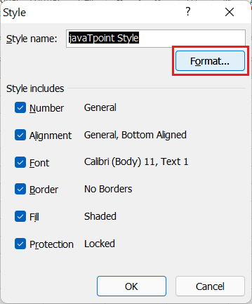
  In the above image, we can notice that the preferences in the style window have changed from the earlier ones. Now, it displays the preferences that we choose from the Format Cells dialogue box.
• After verifying the selected formatting preferences from the Style window, we need to click on the OK button to save our custom style in the active workbook. We can uncheck the checkbox of any format settings we don’t want to use from the Styles window before clicking on the OK button.
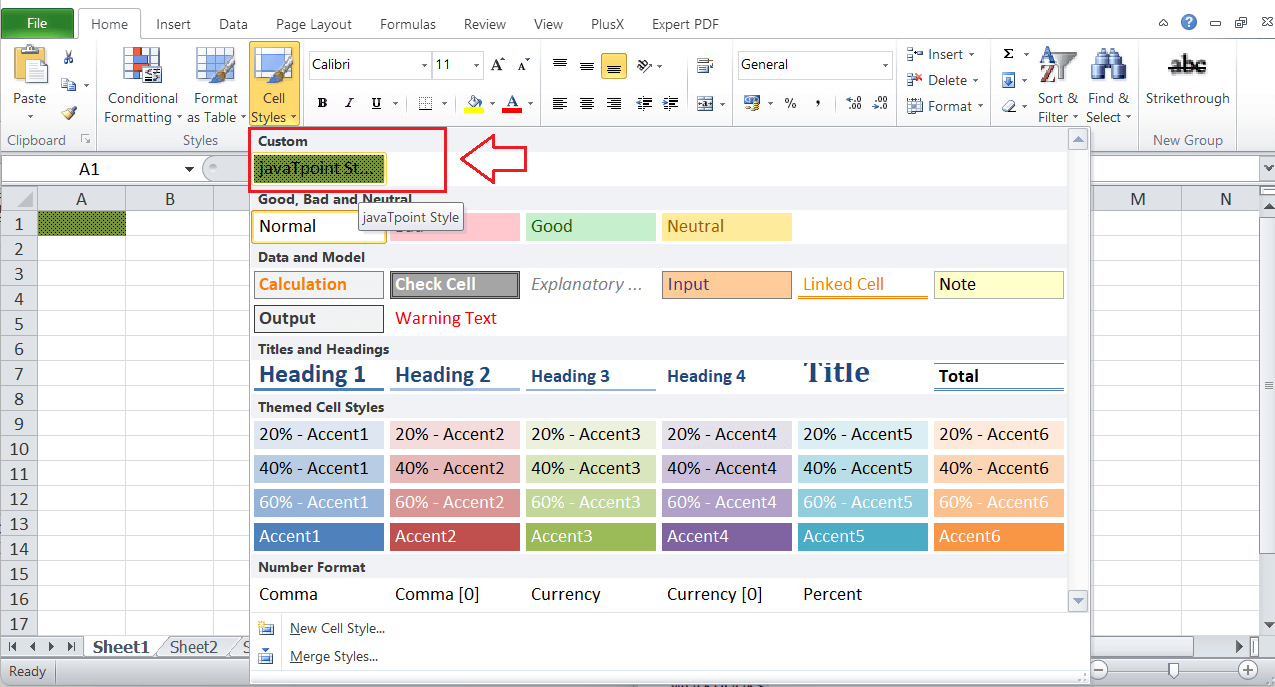
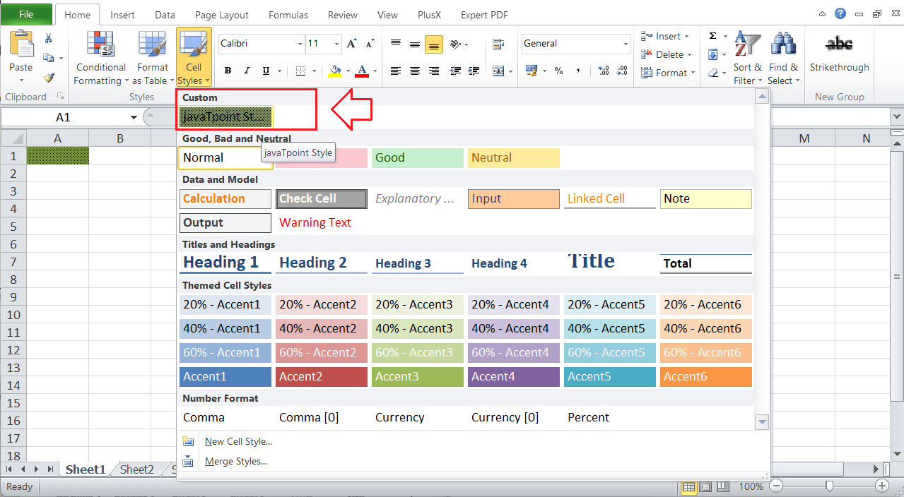
• After creating the custom style, we can access the same by going to Home > Cell Styles > Custom. We will get our saved styles at the top of the style selection window under the Custom option, as shown below:
  
  We can click on our created style, and it will be applied to the selected cells within the current workbook.

Note: When we create a custom style in Excel, the style is saved within the workbook. This means that we can access our created style in all the sheets of the current workbook only, not on other workbooks.

How to merge or export cell styles from one Workbook to another?

As discussed above, the custom cell style we create is saved within the respective workbook only. Therefore, we need to merge cell styles to use the same style with other workbooks, which typically copies the applied style from one workbook to another.

We can perform the following steps to merge or export cell style from one workbook to another:

• First, we need to open both the workbooks: the one from which we want to copy/ merge cell style and another to which we want to apply the style.
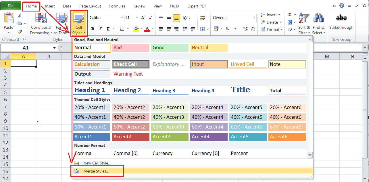
• Next, we need to go to the workbook to which we are going to apply a style. After that, we must navigate the Home > Cell Styles and click on the ‘Merge Styles‘ option, as shown below:
  
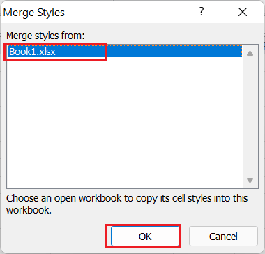
• After clicking on the Merge Style option, Excel displays a list of other workbooks running in the background. We can select the workbook name from which we want to merge the style into our current workbook. After selecting the desired workbook, we must click the OK
  
  In the above image, we are merging the style from Book1.xlsx to Book2.xlsx.
  After merging the style into our desired workbook, we can access it from Home > Cell Styles > Custom.
  

How to Edit a Cell Style?

Excel also enables users to edit the cell styles as per their choice. We can edit our custom styles as well as the existing styles in Excel. For this, we need to go through the following steps:

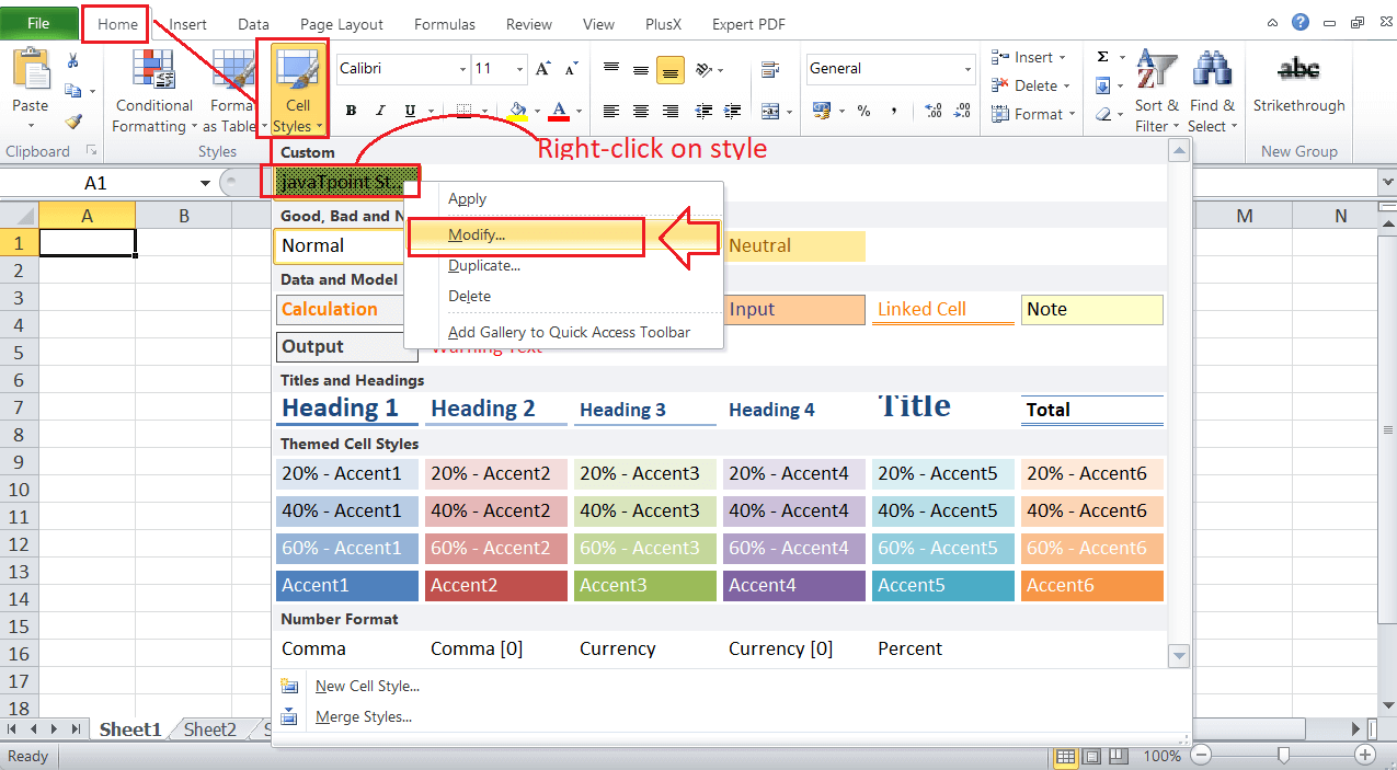
• First, we need to go to Home > Cell Styles and press the right-click button on the style we want to edit. Next, we must click the Modify option from the list, as shown below:
  
• After clicking the Modify option, Excel launches the Style window and displays the current preferences of formatting saved in the corresponding style. Since we want to edit the style, we need to click the Format button from the Style window.
  
• In the Format Cells dialogue box, we can change formatting using their respective tabs within the Format Cells window. Once we have edited the formatting preferences, we need to click the OK button to return to the Style window.
  
• Lastly, we need to click the OK button from the Style window to save all the changes within the selected style. We can also input a new name for the modified style before clicking the OK button.
  
  Similarly, we can use the other options from the right-click menu list to perform related actions, such as applying a style, duplicating it, deleting a style, etc.
  

How to remove/ clear Cell Styles in Excel?

If we don’t like the style or we want to remove the applied style from our workbook completely, it only takes a few steps to follow.

First, we need to select all those cells or a range of cells from which we are willing to remove the applied style. Next, we need to go to the Home tab and click the Cell style icon. In the next window, we need to click the ‘Normal‘ style located near the top under Good, Bad and Neutral. It looks like this:

Clicking on the ‘Normal’ option removes any applied style from the selected cells within the active workbook.

Quick Keyboard Shortcuts for Cell Styles

The keyboard key combination or shortcut is the fastest way to access any specific features or commands in Excel. Excel has predefined shortcuts for most of the built-in features. Unfortunately, we don’t have any definite key combination for cell styles in Excel. However, the Alt key method works perfectly.

Whenever we press the Alt key while the Excel window is active, we activate the quick shortcut keys of Excel tools or commands. Excel then displays specific key (s) on built-in tools within the active window. We only need to press the combination of keys one after another to move through Excel tools or features sequentially.

To access the cell styles in Excel, we need to use the Alt key followed by the ‘H’ and ‘J’ keys, i.e., «Alt + H + J». The Alt key activates the quick shortcuts keys, the H key navigates the Home tab, and the J key selects the Cell Styles option from the ribbon.

After pressing the shortcut key combination, we can use the arrow keys to select the desired style and hit the Enter key to apply.

For other cells styles options, we need to use the following shortcuts:

Action	Shortcut Key
New Cell Style	Alt + H + J + N
Merge Style	Alt + H + J + M

---