
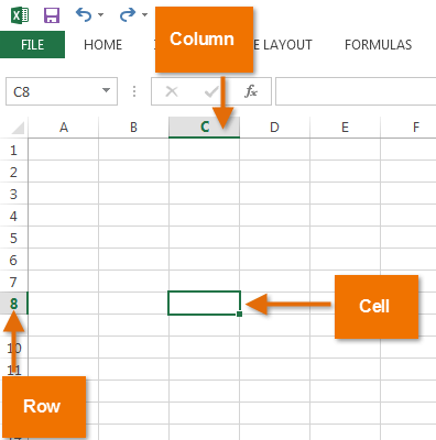
A cell is the storage unit in a spreadsheet program like Microsoft Excel or Google Sheets. Cells are the boxes in a spreadsheet that may contain data. The cells in a spreadsheet are organized within a column and row in the worksheet, and can be formatted for aesthetics or visibility.
Instructions in this article apply to Excel 2019, 2016, 2013, 2010; Excel for Microsoft 365; Excel Online; Excel for Mac; and Google Sheets.
Spreadsheet Cell Types
Cells hold four types of information (also called data types):
- Numbers that can include formulas, dates, and times.
- Text, often referred to as text strings or just strings.
- Boolean values of TRUE or FALSE.
- Errors including #NULL!, #REF!, and #DIV/0! that indicate a problem.
What Are Cell References?
Cell referencing is a system that identifies data and gives it an address so that data can be located in a spreadsheet. A cell reference is used in spreadsheets to identify individual cells and is a combination of the column letter and row number where it is located.
To write a cell reference, start with the column letter and end with the row number, such as A14 or BB329. In the image above, the word Household is located in cell F1 and the highlighted cell is G7.
Cell references are used in formulas to reference other cells. For example, instead of entering the number $360 into a formula found in cell D1, enter a reference to cell G5. When a cell reference is used, if the data in cell G5 changes, the formula in cell D1 also changes.
Cells Can Be Formatted
By default, all cells in a worksheet use the same formatting, but this makes large worksheets containing lots of data difficult to read. Formatting a worksheet draws attention to specific sections and makes data easier to read and understand.
Cell formatting involves making changes to the cell, such as changing the background color, adding borders, or aligning the data in the cell. In contrast, number formatting deals with the way numbers in the cells are displayed, for example, to reflect a currency or percent.
Displayed vs. Stored Numbers
In both Excel and Google Sheets, when number formats are applied, the number that displays in the cell may differ from the number that is stored in the cell and used in calculations.
When formatting changes are made to numbers in a cell, those changes affect the appearance of the number and not the number itself.
For example, if the number 5.6789 in a cell is formatted to display only two decimal places (two digits to the right of the decimal), the cell displays the number as 5.68 due to rounding of the third digit.
Calculations and Formatted Numbers
When using formatted cells of data in calculations, the entire number, in this case, 5.6789, is used in all calculations, not the rounded number appearing in the cell.
How to Add More Cells to a Worksheet
A worksheet has an unlimited number of cells, so you don’t need to add more to the sheet. But, you can add data inside the spreadsheet by adding a cell or group of cells between other cells.
To add a cell to a worksheet:
-
Right-click or tap-and-hold the cell location where you want to add a cell.
-
In Google Sheets, select Insert cells, then choose Shift right or Shift down. This moves every cell in that direction one space and inserts a blank cell in the selected area.
In Excel, choose Insert, then choose either Shift cells right, Shift cells down, Entire row, or Entire column. Select OK to insert the cell.
If you select more than one cell, the program inserts that many cells into the worksheet. For example, highlight one cell to insert just one cell or highlight five cells to add five cells to that location.
-
The cells move and blank cells are inserted.
Delete Cells and Cell Contents
Individual cells and their contents can be deleted from a worksheet. When this happens, cells and their data from either below or to the right of the deleted cell move to fill the gap.
-
Highlight one or more cells to be deleted.
-
Right-click the selected cells and choose Delete.
-
In Excel, choose either Shift cells left or Shift cells up, then select OK. The menu shown here is one way to remove rows and columns.
In Google Sheets, choose Shift left or Shift up.
-
The cells and the corresponding data are removed.
To delete the contents of one or more cells without deleting the cell, highlight the cells and press Delete.
FAQ
-
How do you reference a cell in another Google spreadsheet?
You can use Google Sheets to reference data from another sheet. First, place your cursor in the cell where you want the data and type an equal (=) sign. Next, go to the second sheet, select the cell you want to reference, and press Enter.
-
How do you change cell size in a Google spreadsheet?
To change cell sizes, you can resize rows or columns. One way to do so is with the mouse. Place the mouse pointer on the boundary line between columns or rows, then hold down the left mouse button and drag the double-headed arrow to the desired row or column size.
-
How do you change cell color in a Google spreadsheet?
Select the cell or range of cells to change. Next, select the Fill color icon in the menu bar, and choose the color you want to use.
Thanks for letting us know!
Get the Latest Tech News Delivered Every Day
Subscribe
![]()
Excel Cell

Cell is an Object of Excel Sheet to enter information. It represents with Column Name followed by Row Number. The address of the First Cell in the Excel Sheet is A1 (A is the First Column and 1 is the first Row in Excel sheet). The format of an Excel spread sheet looks like a Table and the intersection of Rows and Columns formats blocks (boxes), each of these small blocks are called Cells in Excel.
How to enter data in a Cell
You can select any Cell in the Excel and press F2 function key to make the Cell editable. Then enter the data using your keyboard in the Cell. You can also double click on a Cell to make it to data entry mode.
What kind of information we can enter in a Cell
We can enter text, numbers, dates, formulas, images, chars, icons and special characters in Excel Cells. We can perform mathematical and logical operations based on our requirements. We can also format the Cell with font styles, colors, number formats,etc.
| Type of Data | Approach to Enter in Excel |
|---|---|
| Enter Date in excel | Use Shortcut key CTRL+ ; (Control and Semicolon) to enter date in Excel. |
| Enter formula in excel | Double Click on any Cell and start with = and enter your formula expression. |
| Enter time in excel | You can use TIMEVALUE(time_text) function to accept the Time. Or you can formate the cell into required time format “h:mm:ss AM/PM”, and enter time value in the cell. |
| Enter today’s date in excel | You can use Ctrl+ ; Shortcut key to enter todats Date in Excel. |
| Enter a checkmark in excel | You can use Char(252) function or Alt+0252 to enter Check Box Character and Change Font of the Cell to Wingdings. |
| Enter a drop down list in excel | Goto Data tab in the Ribbon menu and Clcik on the Data Validation Command to enter Drop down List. |
| Enter 20 digit number in excel | Start with ‘ (apostrophe) and enter the number or format the cell as Text, the number will save as string. |
| Enter a checkbox in excel | Use alt code 0252 and format font to Wingdings. Alternatively, use Symbol command in Insert menu. |
Merge Split (Un Merge) Cells
We have following options and tools in the Excel to merge and unmerge (split) the cells in Excel. You use it based on your requirement.
How to Merge Cells in Excel ?
Follow the below steps to merge the Cells in Excel:
- Select the required range of cells in the sheet
- Go to Home tab in the Ribbon Menu
- Press the ‘Merge Cells‘ Command to merge the Cells.
How to Split Merged Cells in Excel?
Follow the below steps to split the merged Cells in Excel:
- Select the merged cell in the sheet
- Go to Home tab in the Ribbon Menu
- Press the ‘Merge Cells‘ Command to split the cells.
How to Merge Data in Two or More Cells in Excel?
Follow the below steps to merge the data in multiple Cells in Excel:
- You can use the Concatenate Formula to Merge the Cells. For example, =Concatenate(A1,B1)
- You can use concatenate operator & to merge the cell data. For example, =A1&B1
How to Change Excel Cell Size?
You can follow the one of the method to increase the size of the cell in Excel.
- By increasing the width of the column
- Increase the height of the Row
- Increase the font size to make the cell bigger
- merge multiple Cells to make one large size cell
How to Split Data in a Cell in Excel?
Follow the below steps to split the data in a Cell into multiple Cells and Columns:
- Select the required Cell or Column to Split
- Go to Data tab in the Excel Ribbon menu
- Click on the ‘Text to Column’ command in the Data tools group
- Choose and Delimited character or fixed with option to split the data.
How to Extract the Text from Excel Cell?
Follow the below steps to split the data in a Cell into multiple Cells and Columns:
- Select the required Cell or Column to Split
- Go to Data tab in the Excel Ribbon menu
- Click on the ‘Text to Column’ command in the Data tools group
- Choose and Delimited character or fixed with option to split the data.
Lock and Unlock Cells in Excel
We need to protect our data in Excel to hide it from others users. We can use built in Excel tools to lock and unlock the Cells.
How to Lock Excel Cells?
You can lock entire sheet or specific range of cells in the Excel. Follow the below steps to lock the required Cells in the Excel.
- Select the required range of cells to lock (By default Excel cells are locked)
- Then Go to Review Tab in the Excel Ribbon menu
- Click on the ‘Protect Sheet’ command available in the Protect Group.
- Choose the Required things to restrict and enter the password to protect
- And confirm it and press OK to lock it.
How to Un Lock Excel Cells?
Follow the below steps to unlock the cells in Excel. Make sure you have the password to unlock the sheet.
- Go to Review Tab in the Excel Ribbon menu
- Click on the ‘Unprotect Sheet’ command available in the Protect Group.
- Enter the password to un lock the sheet
- Select the required range of cells to un lock.
- Right Click on it and press Format Cells command
- Un select the Locked check mark in the Protection Tab
- Now you can reset the password (if required)
Removing Text from Cells
You can select the required cells to remove the text, press delete key on your keyboard. Excel stores verity of data in Cells, you can follow the below methods to remove the required data from Cells.
| Data | Approach to remove |
|---|---|
| Text | Click Delete Button or Press the Clear Contents command from Editing Tools in Home Tab. |
| Format | Press Clear Formats command from Editiong tools to delete only Formats of the Cells. |
| Comments | Press Clear Comments command from Editiong tools to delete only Comments in the Cells. |
| Delete Everything | Press Clear All command from Editiong tools to delete everything in Cells. |
How to Remove Specific Text From Excel Cell
You can follow the one the following methods to remove specific text from Excel Cells.
- One Cell: You can double click on the cell and select the required text and press delete button from your keyboard.
- Multiple Cells or Columns: You can select entire range of cells and use find and Replace Dialog (Ctrl+H) to remove the specific text (Find What:= your text, Leave blank in the Replace with: text box)
- Part Of Text Criteria: You can use formulas (Mid, Find,Len,Trim) to remove the text based on specific criteria or to Remove Part Of Text From Excel Cell.
How to New Line In Excel Cell
Press Alt+Enter to add new line in Excel. You can use Char(10) with Excel Formula.
Fill Color in Excel Cells
You can fill single or multiple color to set the background colors of the Excel Cells. You fill Solid color or Gradients Color.
- Standard Colors: You can select any cell and go to the Home tab and click on the fill color control (color bucket icon) to set the standard colors in Excel.
- Theme Colors: You can use the one of the colors from Excel Theme Styles, All the cells will change automatically when you change color theme.
- Gradient Colors: You can set Multiple color shading within a single cell using Gradient Effects in Excel. Click on the Format Cells command from the right click menu. And go to Fill Tab and press the Fill effects to set the Cells gradient colors. You can use this option to Split a cell in excel with two or three colors
Cell in Excel Object Model
Cell is a child object of Worksheet. Worksheet is a collection of all cells in the worksheet. Portion of the spreadsheet (One or group of Cells) is called Range in Excel. Here is the Object Model of Excel Cell.

How to Refer a Cell
We use Column Name followed by Row Number to refer a Cell in Excel. For example, C5 is the intersection area of Column C and Row 5. Here C5 is called the address of the Cell. There are two types of methods we can use to refer a Cell.
- Relative Reference: The address of the Cell will change relatively while performing the Excel Operations. It is the default reference type and we can refer as A1 to refer the first cell of a sheet.
- Absolute Reference: The address of the Cell will be fixed and will not change while performing Excel Operations like Copying, Dragging and Auto filling the Cells. We can put $ symbol to make the Row or Column Absolute. For Example, $C$5 is the absolute reference of the cell A5.
We refer the cells to use the data of any cell in other cells and objects. We can use Relative reference, Absolute reference or both combined based on our requirement.
For Example:
=$D$5: will lock both Column and Row, Both Column and Rows are Absolute.
=$D5: will lock Column and will not lock the Row, Column is Absolute and Row is Relative.
=D$5: will lock Row and will not lock the Column, Row is Absolute and Column is Relative.
= D5: Both Column and Rows are Relative.
What is an Active Cell?
A Cell which is currently selected in the Active Sheet of the Active Window is called Active Cell. ActiveCell is an Object of the Worksheet Object , we can use ActiveCell to deal with the currently selected cell of the active worksheet.
For Example:
- We can Enter the data in the Active Cell by typing from keyboard. You can use ActiveCell.Value=10 in Excel Macros.
- We can Format the Active Cell using builtin tools, You can format using Excel Macros like ActiveCell.Font.Bold

© Copyright 2012 – 2020 | Excelx.com | All Rights Reserved
Page load link
Updated: 02/07/2022 by
A cell may refer to any of the following:
1. A cell is the intersection where a row and a column meet on a spreadsheet that starts with cell A1. In the following example, a highlighted cell is shown in a Microsoft Excel spreadsheet. D8 (column D, row  is the highlighted cell that’s also known as the cell address and cell reference. Any modifications made while this cell is highlighted will be limited to this cell in the worksheet.
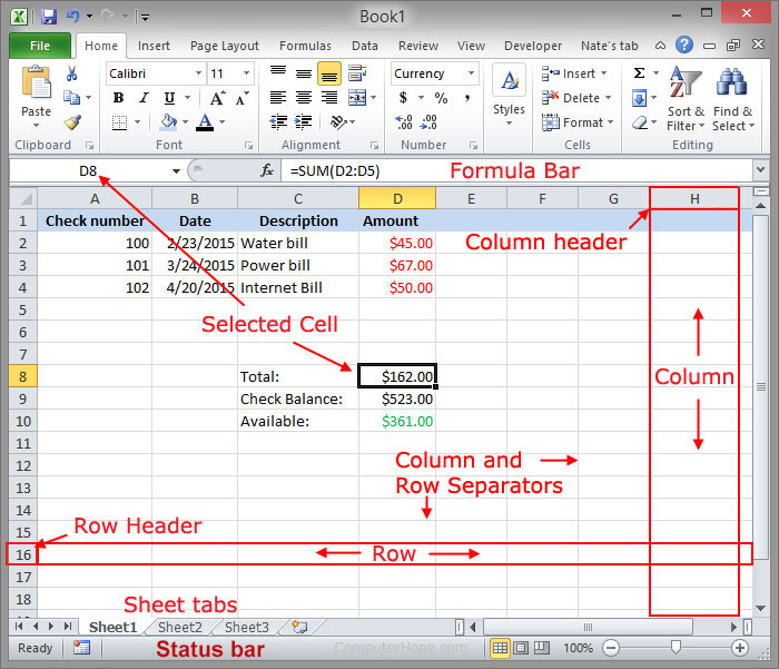
Here, D8 is the active cell. In the formula bar, you can see that the cell content is =SUM(D2:D5). This formula evaluates the result of $162.00 by calculating the sum of the values stored in cells D2 through D5.
Each cell in a spreadsheet can contain any value that can be called using a relative cell reference or called upon using a formula.
- How can you determine the cell reference?
- How do the rows and columns increase?
- How to move between cells.
- Related information.
How can you determine the cell reference?
While moving in a spreadsheet with the keyboard arrow keys or by clicking a cell with the mouse, the cell reference (cell address) is updated. Also, the column and row headers are highlighted. In the picture above, you can see the «D» column, and the «8» row is highlighted in yellow.
How do the rows and columns increase?
When you first open the spreadsheet, the active cell is always placed in the first column (column «A»). As you move to the right, the columns are increased by going through the English alphabet. So, pressing the right arrow key once moves the active cell into the «B» column, pressing the right arrow again moves the active cell into the «C» column, etc. When you get to the last letter of the alphabet («Z»), the columns become two letters with the «AA» column, then «AB,» «AC,» etc. After getting to «AZ,» the columns become «BA,» «BB,» «BC,» etc. If you were to get to «ZZ,» the next column would increase to three letters and start with «AAA,» then «AAB,» «AAC,» etc.
Rows are increased numerically, starting with the first row of number «1.» Pressing the down arrow key would increase the row to «2,» and pressing it again would increase the row to «3.»
- How many sheets, rows, and columns can a spreadsheet have?
Tip
See our spreadsheet definition for further information on using spreadsheets.
How to move between cells
To move between cells in a spreadsheet, click the cell where you want to move to or use the arrow keys to move up, down, left, and right one cell. You can also use the page up and page down keys to move one page at a time.
- Excel up and down arrow keys move page instead of cell.
Other keyboard shortcuts
In addition to moving between cells using the arrow keys, you can also use the following keyboard shortcuts.
- F5 — The F5 function key lets you go to a specific cell. For example, you could press F5, type «n9» and press Enter to go to cell N9.
- Tab — Press Tab moves one cell to the right.
- Shift+Tab — Move one cell to the left.
- Home — Move to the first cell in the row.
- Ctrl+Home — Go to the first cell in the spreadsheet (A1).
- Ctrl+End — Go to the last cell with data in the worksheet.
2. Like a spreadsheet cell, a cell is a section within an HTML table that is created using the HTML <td> tag.
3. Cell is another name for a cell phone.
4. A cell refers to a unit of data that is transferred over an ATM network.
5. Cell is the geographical area that a cell tower covers for cell phone reception. It is often measured in square miles and may overlap with another cell tower’s cell.
Cel, Range, Relative cell reference, Row, Spreadsheet, Spreadsheet terms
Last update on August 19 2022 21:50:34 (UTC/GMT +8 hours)
What is a cell ?
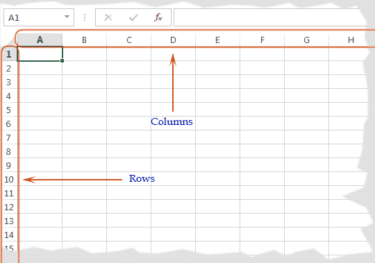
The worksheet of a workbook in Excel 2013 are made up of thousands of rectangles, are called cells. A cell is the intersection of a row and a column. Columns are identified by letters (A, B, C…), whereas rows are identified by numbers (1, 2, 3…). Here is the picture below to explain the rows and columns.
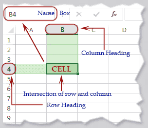
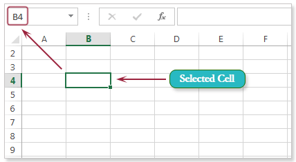
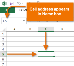
Each cell has its own name, or cell address, a combination of column and row. Here in the example below, the selected cell is the intersection or column B and row 4, so the cell address is B4. The cell address will also appear in the Name box. The another way to understand the selected row and column that, a cell’s column and row headings are highlighted when the cell is selected.
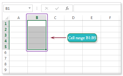
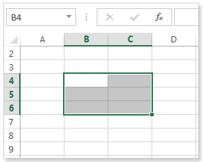
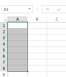
Multiple cells can also be selected at the same time. A group of cells is known as a cell range. A range of cells can be referred by using the cell addresses of the first and last cells and separated by a colon. Here in the picture below a cell range that included cells B1, B2, B3, B4, and B5 would be written as B1:B5.
 .
.
Select a cell:
To input new data into a cell or edit cell content, you have to select the desired cell and click the mouse into your desired cell to select it.
A border will appear around the selected cell, and the column and row heading associated with the selected will be highlighted. The cell will remain selected until you click another cell in the worksheet.
A cell can also be selected using the arrow keys on your keyboard.
Select a range of cells:
Sometimes we need to select a range of cells, then you need to press and hold the left mouse button, and drag the mouse until all of the adjoining cells you wish to select are highlighted and release the mouse.
The cells will remain selected until you click another cell in the worksheet.
Merge Cells:
Two or more cells can be merged in one depends on your requirement.
Merge multi Cells:
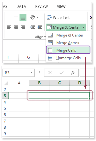
You can selecte multi cells, and then click Merge & Center in the alignment group of ribbon menu. Then choose from the option.
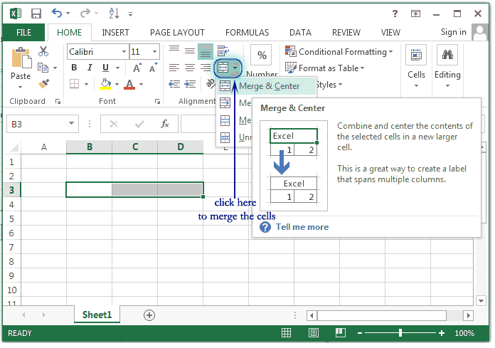
Here in the example above select B3 to D3 and click on Merge & Center. Three cells merge and make one cell. Here is the picture below.
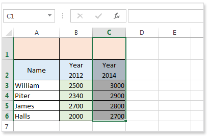
Delete a cell:
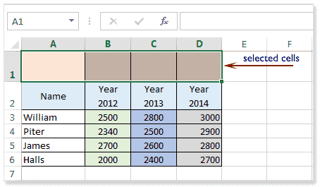
There is an important different between deleting the content of a cell and deleting the cell itself. If you want to delete a cell or cells , the cells below and right of the selected cell(s) will shift up or left and replace the deleted cells.
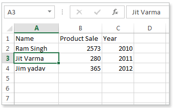
Select the cell(s) which you want to delete.Then select the Delete command under cell group from the Home tab of the Ribbon, and click on Delete Cells. Here is the example below.
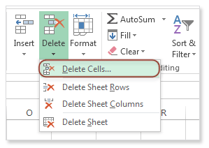
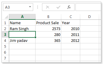
The picture below shows that the, cells below have been shifted up.
Here is another example
The picture below shows that the, cells right have been shifted left.
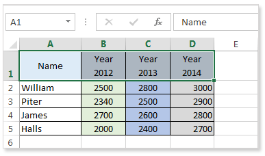
As a cell is associated with a row and column, so at the time of deletion of a cell or cells the four option may come. These are —
A cell may be deleted by replacing the below cell to up or by replacing the right cell to left.
The entire row or rows associated with the cell or cells may be deleted.
The entire column or columns associated with the cell or cells may be deleted.
Here is the picture below.
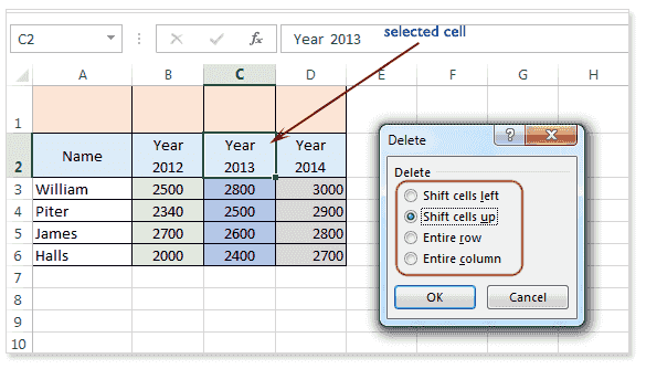
The above picture shows that, the C2 cell is selected and this cell is associated with column C and row 2. So the C2 cell can be deleted by C3 up or by shifting the D2 cell left or the entire C column can be deleted or entire 2 row can be deleted.
Cell content
Information entered into a spreadsheet will be stored in a cell. Each cell can contain several different kinds of content, including text, formatting, formulas, and functions.
Text type data
Cells can contain text, such as letters, numbers, and dates.
Insert content into cell
Click a cell to select it.
Type content into the selected cell, then press Enter on your keyboard. The content will appear in the cell and the formula bar. You can also input and edit cell content in the formula bar.
Copy and paste cell content
Excel allows you to copy content that is already entered into the spreadsheet and paste that content into other cells.
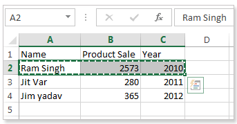
Select the cell(s) that you want to copy. Then click the Copy command under the Home tab or press Ctrl+C on the keyboard.
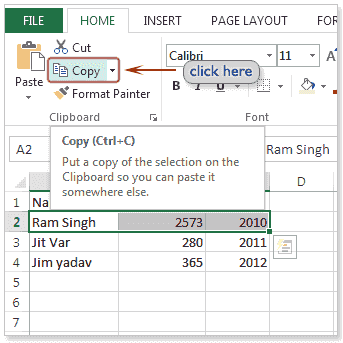
The copied cells will now have a dashed box around them. Here is the picture below after click the copy command.
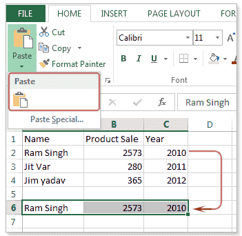
Now select the cell where you wish to paste the content and click on paste command. Here is the picture below.
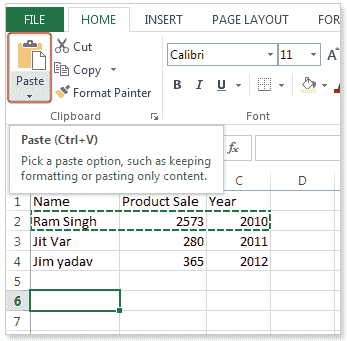
Click the arrow of the Paste command under the Home tab, or press Ctrl+V on the keyboard.
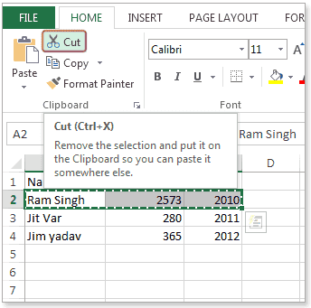
Select the cell or cells you want to cut then click the Cut command under the Home tab, or press Ctrl+X on the keyboard. The cells will now have a dashed box around them.
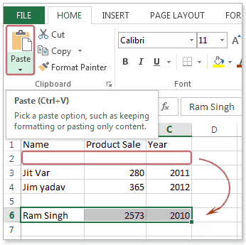
Select the cells where you wish to paste the content.
Click the Paste command under Home tab, or press Ctrl+V on the keyboard. The content from the cells which you have selected for cut will move to the desired location. See the picture below.
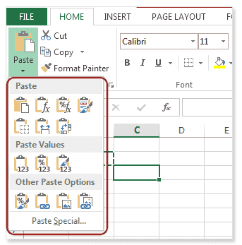
To access more paste options:
To get various types of paste options, click the drop-down arrow on the Paste command. Here is the picture below.
Instead of choosing commands from the Ribbon, you can get the options quickly by right-clicking the mouse on the cell where you want to paste the copied or cut content.
Drag and drop cells:
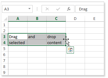
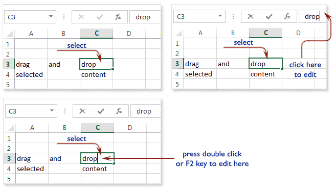
Another way to move the content instead of cut command is to drag and drop cells to move the contents. Select the range A3:C4, and place the mouse pointer at any edge of selected area. A four-headed arrow will appear, then press and hold the mouse and drag your desired place and release the mouse, the selected content will move. Here is the picture below.
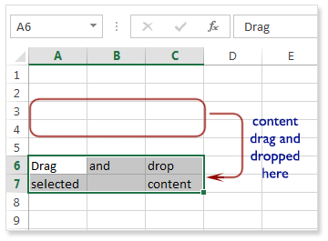
The picture below shows that the content of A3 to C4 have been moved into A6 to C7.
Delete cell content:
Select the cell with content which you want to delete.
Press the Delete or Backspace key on the keyboard. The cell’s contents will be deleted.
Edit cell content
The content of a cell can be modified by the various way. You can do it by double clicking the cell where the content located, or select the cell and click on formula bar and edit the content or select the cell and press the F2 function key from the keyboard to edit the content of the cell.
Previous: Backstage View — Excel 2013
Next:
Cell References in Excel
Lesson 7: Cell Basics
/en/excel2013/saving-and-sharing-workbooks/content/
Introduction
Whenever you work with Excel, you’ll enter information—or content—into cells. Cells are the basic building blocks of a worksheet. You’ll need to learn the basics of cells and cell content to calculate, analyze, and organize data in Excel.
Optional: Download our practice workbook.
Understanding cells
Every worksheet is made up of thousands of rectangles, which are called cells. A cell is the intersection of a row and a column. Columns are identified by letters (A, B, C), while rows are identified by numbers (1, 2, 3).
 A cell
Each cell has its own name—or cell address—based on its column and row. In this example, the selected cell intersects column C and row 5, so the cell address is C5. The cell address will also appear in the Name box. Note that a cell’s column and row headings are highlighted when the cell is selected.
 Cell C5
You can also select multiple cells at the same time. A group of cells is known as a cell range. Rather than a single cell address, you will refer to a cell range using the cell addresses of the first and last cells in the cell range, separated by a colon. For example, a cell range that included cells A1, A2, A3, A4, and A5 would be written as A1:A5.
In the images below, two different cell ranges are selected:
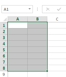
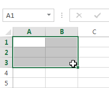
- Cell range A1:A8
 Cell range A1:A8
 - Cell range A1:B8
Cell range A1:B8
If the columns in your spreadsheet are labeled with numbers instead of letters, you’ll need to change the default reference style for Excel. Review our Extra on What are Reference Styles? to learn how.
To select a cell:
To input or edit cell content, you’ll first need to select the cell.
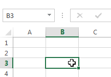
- Click a cell to select it.
- A border will appear around the selected cell, and the column heading and row heading will be highlighted. The cell will remain selected until you click another cell in the worksheet.
 Selecting a single cell
 will appear around the selected cell, and the column heading and row heading will be highlighted. The cell will remain selected until you click another cell in the worksheet.
You can also select cells using the arrow keys on your keyboard.
To select a cell range:
Sometimes you may want to select a larger group of cells, or a cell range.
- Click, hold, and drag the mouse until all of the adjoining cells you want to select are highlighted.
- Release the mouse to select the desired cell range. The cells will remain selected until you click another cell in the worksheet.
 Selecting a cell range
Cell content
Any information you enter into a spreadsheet will be stored in a cell. Each cell can contain different types of content, including text, formatting, formulas, and functions.
- Text
Cells can contain text, such as letters, numbers, and dates. Cell text
 - Formatting attributes
Cells can contain formatting attributes that change the way letters, numbers, and dates are displayed. For example, percentages can appear as 0.15 or 15%. You can even change a cell’s background color. Cell formatting
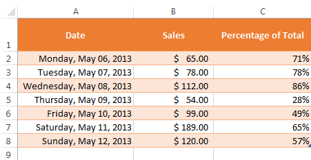
 - Formulas and functions
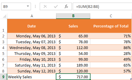
Cells can contain formulas and functions that calculate cell values. In our example, SUM(B2:B8) adds the value of each cell in cell range B2:B8 and displays the total in cell B9. Cell formulas
To insert content:
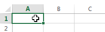
- Click a cell to select it.
 Selecting cell A1
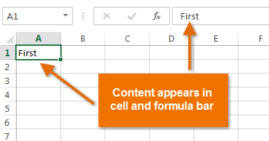
 - Type content into the selected cell, then press Enter on your keyboard. The content will appear in the cell and the formula bar. You can also input and edit cell content in the formula bar.
 Inserting cell content
To delete cell content:
- Select the cell with content you want to delete.
 Selecting a cell
 - Press the Delete or Backspace key on your keyboard. The cell’s contents will be deleted.
 Deleting cell content
You can use the Delete key on your keyboard to delete content from multiple cells at once. The Backspace key will only delete one cell at a time.
To delete cells:
There is an important difference between deleting the content of a cell and deleting the cell itself. If you delete the entire cell, the cells below it will shift up and replace the deleted cells.
- Select the cell(s) you want to delete.
 Selecting a cell to delete
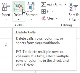
 - Select the Delete command from the Home tab on the Ribbon.
 Clicking the Delete command
 - The cells below will shift up.
 Cells shifted to replace the deleted cell
To copy and paste cell content:
Excel allows you to copy content that is already entered into your spreadsheet and paste that content to other cells, which can save you time and effort.
- Select the cell(s) you want to copy.
 Selecting a cell to copy
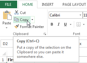
 - Click the Copy command on the Home tab, or press Ctrl+C on your keyboard.
 Clicking the Copy command
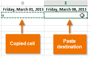
 - Select the cell(s) where you want to paste the content. The copied cells will now have a dashed box around them.
 Pasting cells
 - Click the Paste command on the Home tab, or press Ctrl+V on your keyboard.
 Clicking the Paste command
 - The content will be pasted into the selected cells.
 The pasted cell content
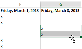
To cut and paste cell content:
Unlike copying and pasting, which duplicates cell content, cutting allows you to move content between cells.
- Select the cell(s) you want to cut.
 Selecting a cell range to cut
 - Click the Cut command on the Home tab, or press Ctrl+X on your keyboard.
 Clicking the Cut command
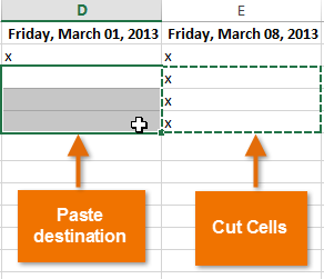
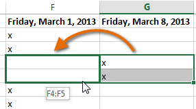
 - Select the cells where you want to paste the content. The cut cells will now have a dashed box around them.
 Pasting cells
 - Click the Paste command on the Home tab, or press Ctrl+V on your keyboard.
Clicking the Paste command
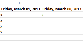
- The cut content will be removed from the original cells and pasted into the selected cells.
 The cut and pasted cells
To access more paste options:
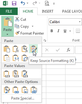
You can also access additional paste options, which are especially convenient when working with cells that contain formulas or formatting.
- To access more paste options, click the drop-down arrow on the Paste command.
 Additional Paste options
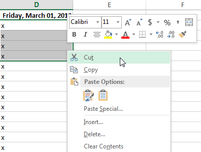
Rather than choose commands from the Ribbon, you can access commands quickly by right-clicking. Simply select the cell(s) you want to format, then right-click the mouse. A drop-down menu will appear, where you’ll find several commands that are also located on the Ribbon.
 Right-clicking to access formatting options
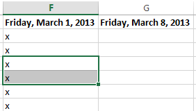
To drag and drop cells:
Rather than cutting, copying, and pasting, you can drag and drop cells to move their contents.
- Select the cell(s) you want to move.
- Hover the mouse over the border of the selected cell(s) until the cursor changes from a white cross to a black cross with four arrows.
 Hovering over the cell border
 - Click, hold, and drag the cells to the desired location.
 Dragging the selected cells
 - Release the mouse, and the cells will be dropped in the selected location.
 The dropped cells
 to a black cross with four arrows
 .
.
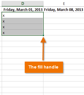
To use the fill handle:
There may be times when you need to copy the content of one cell to several other cells in your worksheet. You could copy and paste the content into each cell, but this method would be time consuming. Instead, you can use the fill handle to quickly copy and paste content to adjacent cells in the same row or column.
- Select the cell(s) containing the content you want to use. The fill handle will appear as a small square in the bottom-right corner of the selected cell(s).
 Locating the fill handle
 - Click, hold, and drag the fill handle until all of the cells you want to fill are selected.
 Dragging the fill handle
 - Release the mouse to fill the selected cells.
 The filled cells
To continue a series with the fill handle:
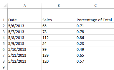
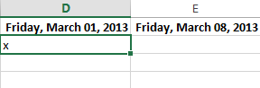
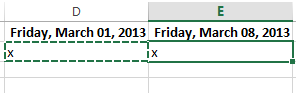
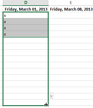
The fill handle can also be used to continue a series. Whenever the content of a row or column follows a sequential order, like numbers (1, 2, 3) or days (Monday, Tuesday, Wednesday), the fill handle can guess what should come next in the series. In many cases, you may need to select multiple cells before using the fill handle to help Excel determine the series order. In our example below, the fill handle is used to extend a series of dates in a column.
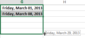 Using the fill handle to extend a series
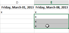
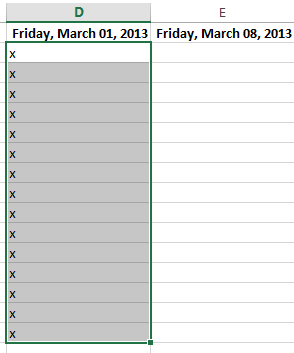
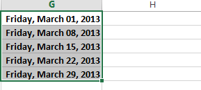 The extended series
You can also double-click the fill handle instead of clicking and dragging. This can be useful with larger spreadsheets, where clicking and dragging may be awkward.
Watch the video below to see an example of double-clicking the fill handle.
To use Flash Fill:
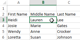
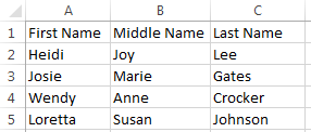
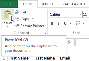
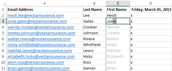
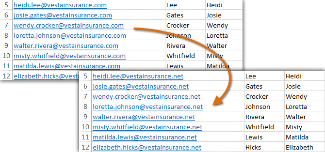
A new feature in Excel 2013, Flash Fill can enter data automatically into your worksheet, saving you time and effort. Just like the fill handle, Flash Fill can guess what type of information you’re entering into your worksheet. In the example below, we’ll use Flash Fill to create a list of first names using a list of existing email addresses.
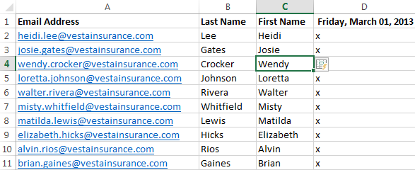
- Enter the desired information into your worksheet. A Flash Fill preview will appear below the selected cell whenever Flash Fill is available.
 Previewing Flash Fill data
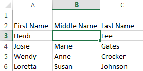
 - Press Enter. The Flash Fill data will be added to the worksheet.
 The entered Flash Fill data
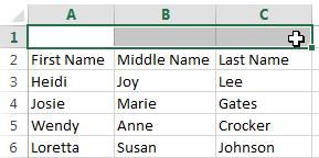
To modify or undo Flash Fill, click the Flash Fill button next to recently added Flash Fill data.
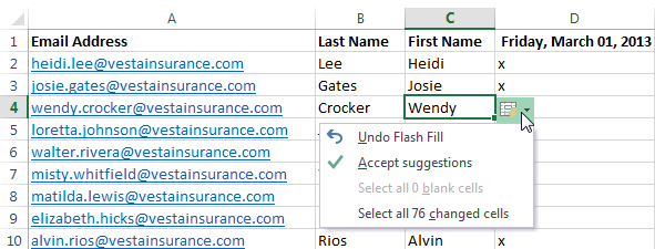 Clicking the Flash Fill button
Find and Replace
When working with a lot of data in Excel, it can be difficult and time consuming to locate specific information. You can easily search your workbook using the Find feature, which also allows you to modify content using the Replace feature.
To find content:
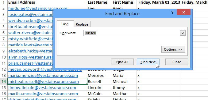
In our example, we’ll use the Find command to locate a specific name in a long list of employees.
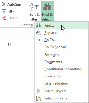
- From the Home tab, click the Find and Select command, then select Find… from the drop-down menu.
 Clicking the Find command
 - The Find and Replace dialog box will appear. Enter the content you want to find. In our example, we’ll type the employee’s name.
- Click Find Next. If the content is found, the cell containing that content will be selected.
 Clicking Find Next
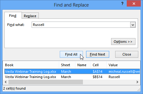
 - Click Find Next to find further instances or Find All to see every instance of the search term.
 Clicking Find All
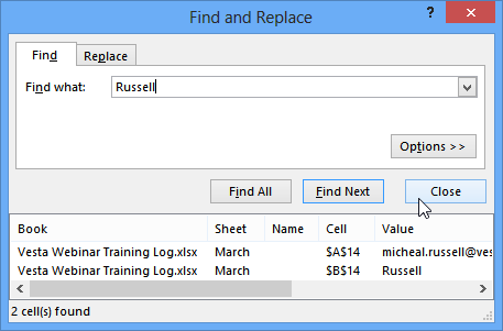
 - When you are finished, click Close to exit the Find and Replace dialog box.
Closing the Find and Replace dialog box
You can also access the Find command by pressing Ctrl+F on your keyboard.
Click Options to see advanced search criteria in the Find and Replace dialog box.
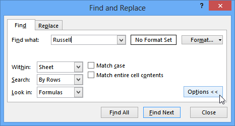 Clicking Options
To replace cell content:
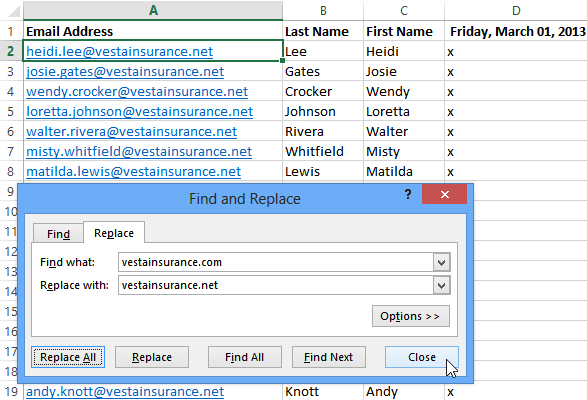
At times, you may discover that you’ve repeatedly made a mistake throughout your workbook (such as misspelling someone’s name), or that you need to exchange a particular word or phrase for another. You can use Excel’s Find and Replace feature to make quick revisions. In our example, we’ll use Find and Replace to correct a list of email addresses.
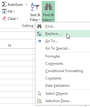
- From the Home tab, click the Find and Select command, then select Replace… from the drop-down menu.
 Clicking the Replace command
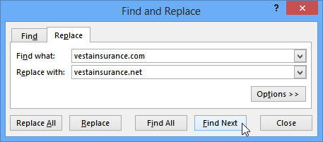
 - The Find and Replace dialog box will appear. Type the text you want to find in the Find what: field.
- Type the text you want to replace it with in the Replace with: field, then click Find Next.
 Clicking Find Next
 - If the content is found, the cell containing that content will be selected.
- Review the text to make sure you want to replace it.
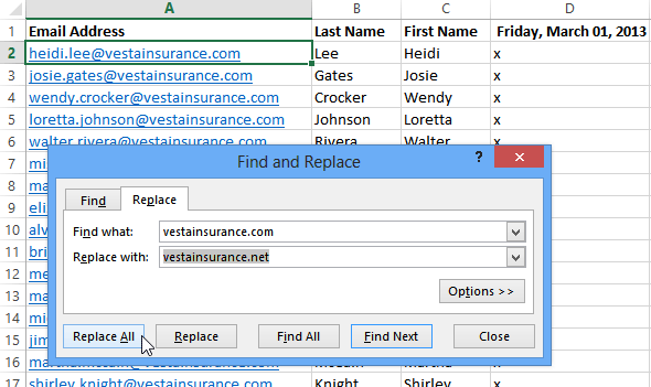
- If you want to replace it, select one of the replace options:
- Replace will replace individual instances.
- Replace All will replace every instance of the text throughout the workbook. In our example, we’ll choose this option to save time.
 Replacing the highlighted text
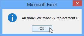
 - A dialog box will appear, confirming the number of replacements made. Click OK to continue.
 Clicking OK
 - The selected cell content will be replaced.
 The replaced content
 - When you are finished, click Close to exit the Find and Replace dialog box.
 Closing the Find and Replace dialog box
Challenge!
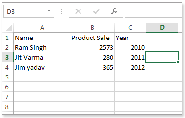
- Open an existing Excel 2013 workbook. If you want, you can use our practice workbook.
- Select cell D3. Notice how the cell address appears in the Name box and its content appears in both the cell and the Formula bar.
- Select a cell, and try inserting text and numbers.
- Delete a cell, and note how the cells below shift up to fill in its place.
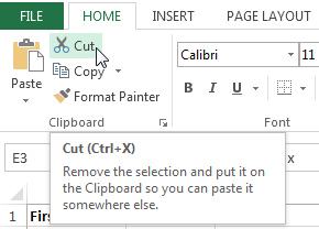
- Cut cells and paste them into a different location. If you are using the example, cut cells D4:D6 and paste them to E4:E6.
- Try dragging and dropping some cells to other parts of the worksheet.
- Use the fill handle to fill in data to adjoining cells both vertically and horizontally. If you are using the example, use the fill handle to continue the series of dates across row 3.
- Use the Find feature to locate content in your workbook. If you are using the example, type the name Lewis into the Find what: field.
/en/excel2013/modifying-columns-rows-and-cells/content/