
![]()
Download Article
![]()
Download Article
This wikiHow teaches you how to create a line of best fit in your Microsoft Excel chart. A line of best fit, also known as a best fit line or trendline, is a straight line used to indicate a trending pattern on a scatter chart. If you were to create this type of line by hand, you’d need to use a complicated formula. Fortunately, Excel makes it easy to find an accurate trend line by doing the calculations for you.
-

1
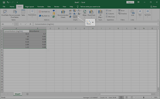
Highlight the data you want to analyze. The data you select will be used to create your scatter chart. A scatter chart is one that uses dots to represent values for two different numeric values (X and Y).
-
2
Click the Insert tab. It’s at the top of Excel.
Advertisement
-
3
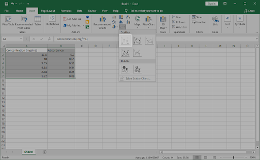
Click the Scatter icon on the Charts panel. It’s in the toolbar at the top of the screen. The icon looks like several small blue and yellow squares—when you hover the mouse cursor over this icon, you should see «Insert Scatter (X, Y)» or Bubble Chart (the exact wording varies by version).[1]
A list of different chart types will appear. -
4
Click the first Scatter chart option. It’s the chart icon at the top-left corner of the menu. This creates a chart based on the selected data.
-
5
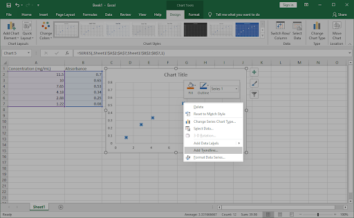
Right-click one of the data points on your chart. This can be any of the blue dots on the chart. This selects all of the data points at once and expands a menu.
- If you are using a Mac and don’t have a right mouse button, hold down the Ctrl button as you click a dot instead.
-
6
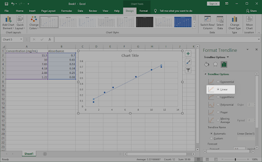
Click Add Trendline on the menu. Now you’ll see the Format Trendline panel on the right side of Excel.
-
7
Select Linear from the Trendline Options. It’s the second option in the Format Trendline panel. You should now see a linear straight line that reflects the trend of your data.
-
8
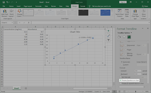
Check the box next to «Display equation on chart.» It’s toward the bottom of the Format Trendline panel. This displays the math calculations used to create the best fit line. This step is optional, but can be useful for anyone viewing your chart who wants to understand how the best fit line was calculated.
- Click the X at the top-right corner of the Format Trendline panel to close it.


Advertisement
Ask a Question
200 characters left
Include your email address to get a message when this question is answered.
Submit
Advertisement
Video
-
While your chart is selected, you can customize its colors and other features by experimenting with the options on the Design tab. Click Change Colors in the toolbar to choose a color scheme, and then scroll through the «Chart styles» options to find one that looks good for your data.
Thanks for submitting a tip for review!
Advertisement
References
About This Article
Article SummaryX
1. Highlight the data for your chart.
2. Click the Insert tab.
3. Click the Scatter icon.
4. Click the first Scatter chart.
5. Right-click one of the data points on the chart.
6. Click Add Trendline.
7. Select «Linear.»
8. Check the box next to «Display equation on chart.»
Did this summary help you?
Thanks to all authors for creating a page that has been read 47,293 times.
Is this article up to date?
Right Click on any one of the data points and a dialog box will appear. Click “Add Trendline”; this is what Excel calls a “best fit line”: 16.
Contents
- 1 How do you find the equation of the line of best fit on Excel?
- 2 How do you make a best fit column in Excel?
- 3 How do I find the line of best fit?
- 4 What is best fit curve?
- 5 How do you use the Logest function?
- 6 How do I make Excel cells fit text?
- 7 How do you do a trend in Excel?
- 8 How do you make a best fit column?
- 9 How do you resize a column to best fit?
- 10 How do I make my Excel spreadsheet fit on one page?
- 11 Does line of best fit have to start at 0?
- 12 Is the line of best fit the same as the regression line?
- 13 What does Logest formula in Excel?
- 14 What is Logest Excel?
- 15 What is the formula of growth in Excel?
- 16 How do you put borders on Excel?
- 17 How do I resize a column in Excel?
- 18 How do you forecast trends?
- 19 How do you go upward and downward trends in Excel?
- 20 How do you perform a trend analysis?
How do you find the equation of the line of best fit on Excel?
To show the equation, click on “Trendline” and select “More Trendline Options…” Then check the “Display Equation on chart” box.
How do you make a best fit column in Excel?
Select the column or columns that you want to change. On the Home tab, in the Cells group, click Format. Under Cell Size, click AutoFit Column Width. Note: To quickly autofit all columns on the worksheet, click the Select All button, and then double-click any boundary between two column headings.
How do I find the line of best fit?
A line of best fit can be roughly determined using an eyeball method by drawing a straight line on a scatter plot so that the number of points above the line and below the line is about equal (and the line passes through as many points as possible).
What is best fit curve?
Curve of Best Fit: a curve the best approximates the trend on a scatter plot. If the data appears to be quadratic, we perform a quadratic regression to get the equation for the curve of best fit. If it appears to be cubic, then we perform a cubic regression.
How do you use the Logest function?
Here are the steps for this function:
- With the data entered, select a five-row-by-two-column array of cells for LOGEST ‘s results.
- From the Statistical Functions menu, select LOGEST to open the Function Arguments dialog box for LOGEST .
- In the Function Arguments dialog box, type the appropriate values for the arguments.
How do I make Excel cells fit text?
Select the cells to which you want to apply ‘Shrink to Fit’ Hold the Control key and press the 1 key (this will open the Format Cells dialog box) Click the ‘Alignment’ tab. In the ‘Text Control’ options, check the ‘Shrink to Fit’ option.
How do you do a trend in Excel?
Add a trendline
- Select a chart.
- Select the + to the top right of the chart.
- Select Trendline. Note: Excel displays the Trendline option only if you select a chart that has more than one data series without selecting a data series.
- In the Add Trendline dialog box, select any data series options you want, and click OK.
How do you make a best fit column?
Automatically adjust your table or columns to fit the size of your content by using the AutoFit button.
- Select your table.
- On the Layout tab, in the Cell Size group, click AutoFit.
- Do one of the following. To adjust column width automatically, click AutoFit Contents.
How do you resize a column to best fit?
Using the “Best Fit” feature in Access, though, you can adjust the width of columns dynamically.
- Click the Microsoft Office ribbon at the top-left corner of the screen. Video of the Day.
- Click the “Records” section.
- Click “More” from the drop-down menu.
- Choose “Column Width.”
- Click “Best Fit.”
How do I make my Excel spreadsheet fit on one page?
Shrink a worksheet to fit on one page
Select the Page tab in the Page Setup dialog box. Select Fit to under Scaling. To fit your document to print on one page, choose 1 page(s) wide by 1 tall in the Fit to boxes. Note: Excel will shrink your data to fit on the number of pages specified.
Does line of best fit have to start at 0?
The line of best fit does not have to go through the origin. The line of best fit shows the trend, but it is only approximate and any readings taken from it will be estimations.
Is the line of best fit the same as the regression line?
The regression line is sometimes called the “line of best fit” because it is the line that fits best when drawn through the points. It is a line that minimizes the distance of the actual scores from the predicted scores.
What does Logest formula in Excel?
In regression analysis, the LOGEST function calculates an exponential curve that fits your data and returns an array of values that describes the curve. Because this function returns an array of values, it must be entered as an array formula.Excel inserts curly brackets at the beginning and end of the formula for you.
What is Logest Excel?
The LOGEST function in Excel is a function used to fit an exponential curve to exponential data. LOGEST is an array formula. Note that while using Microsoft 365, LOGEST is compatible with dynamic arrays and does not require the use of Ctrl + Shift + Enter (CSE).We can use LOGEST to fit a curve to the data.
What is the formula of growth in Excel?
For GROWTH Formula in Excel, y =b* m^x represents an exponential curve where the value of y depends upon the value x, m is the base with exponent x, and b is a constant value.
How do you put borders on Excel?
Here’s how:
- Select a cell or a range of cells to which you want to add borders.
- On the Home tab, in the Font group, click the down arrow next to the Borders button, and you will see a list of the most popular border types.
- Click the border you want to apply, and it will be immediately added to the selected cells.
How do I resize a column in Excel?
Resize columns
- Select a column or a range of columns.
- On the Home tab, in the Cells group, select Format > Column Width.
- Type the column width and select OK.
How do you forecast trends?
7 Tips for Trend Forecasting in Today’s Market
- FIND OUT WHERE YOUR CONSUMER IS GETTING INSPIRED.
- LEARN EVERYTHING YOU CAN ABOUT YOUR CONSUMERS’ PSYCHOGRAPHICS.
- BE REACTIVE.
- FOCUS ON THE CONVERSION.
- UNDERSTAND VISUAL CONSUMPTION.
- UTILIZE THE LATEST TECHNOLOGY.
- HEAR THE COLLECTIVE VOICE.
How do you go upward and downward trends in Excel?
Select the target range of cells and select Manage Rules under the Conditional Formatting button on the Home tab of the Ribbon. In the dialog box that opens, click the Edit Rule button. Adjust the properties, as shown here. You can adjust the thresholds that define what up, down, and flat mean.
How do you perform a trend analysis?
- 1 – Choose Which Pattern You Want to Identify. The first and most obvious step in trend analysis is to identify which data trend you want to target.
- 2 – Choose Time Period.
- 3 – Choose Types of Data Needed.
- 4 – Gather Data.
- 5 – Use Charting Tools to Visualize Data.
- 6 – Identify Trends.
In statistics, a line of best fit is the line that best “fits” or describes the relationship between a predictor variable and a response variable.
The following step-by-step example shows how to create a line of best fit in Excel.
Step 1: Enter the Data
First, let’s enter the following dataset that shows the number of hours spent practicing and the total points scored by eight different basketball players:

Step 2: Create a Scatter Plot
Next, let’s create a scatter plot to visualize the relationship between the two variables.
To do so, highlight the cells in the range A2:B9, then click the Insert tab along the top ribbon, then click the option titled Scatter in the Charts group:

The following scatter plot will automatically be created:

Step 3: Add the Line of Best Fit
To add a line of best fit to the scatter plot, click anywhere on the chart, then click the green plus (+) sign that appears in the top right corner of the chart.
Then click the arrow next to Trendline, then click More Options:

In the Format Trendline panel that appears, click the button next to Linear as the trendline option, then check the box next to Display Equation on chart:

The line of best fit along with the equation for the line will appear on the chart:

Step 4: Interpret the Line of Best Fit
From the chart we can see that the line of best fit has the following equation:
y = 2.3095x – 0.8929
Here is how to interpret this equation:
- For each additional hour spent practicing, average points scored increases by 2.3095.
- For a player who practices zero hours, average points scored is expected to be -0.8929.
Note that it doesn’t always make sense to interpret the intercept value in a regression equation.
For example, it’s not possible for a player to score negative points.
In this particular example, we’re mostly interested in the value for the slope of the regression line which is 2.3095.
Additional Resources
The following tutorials explain how to perform other common tasks in Excel:
How to Perform Simple Linear Regression in Excel
How to Perform Multiple Linear Regression in Excel
How to Calculate R-Squared in Excel
Access for Microsoft 365 Access 2021 Access 2019 Access 2016 Access 2013 Access 2010 Access 2007 MS Graph 2003 More…Less
When you want to add a trendline to a chart in Microsoft Graph, you can choose any of the six different trend/regression types. The type of data you have determines the type of trendline you should use.
Trendline reliability A trendline is most reliable when its R-squared value is at or near 1. When you fit a trendline to your data, Graph automatically calculates its R-squared value. If you want, you can display this value on your chart.
Linear
A linear trendline is a best-fit straight line that is used with simple linear data sets. Your data is linear if the pattern in its data points resembles a line. A linear trendline usually shows that something is increasing or decreasing at a steady rate.
In the following example, a linear trendline clearly shows that refrigerator sales have consistently risen over a 13-year period. Notice that the R-squared value is 0.9036, which is a good fit of the line to the data.
Logarithmic
A logarithmic trendline is a best-fit curved line that is most useful when the rate of change in the data increases or decreases quickly and then levels out. A logarithmic trendline can use negative and/or positive values.
The following example uses a logarithmic trendline to illustrate predicted population growth of animals in a fixed-space area, where population leveled out as space for the animals decreased. Note that the R-squared value is 0.9407, which is a relatively good fit of the line to the data.
Polynomial
A polynomial trendline is a curved line that is used when data fluctuates. It is useful, for example, for analyzing gains and losses over a large data set. The order of the polynomial can be determined by the number of fluctuations in the data or by how many bends (hills and valleys) appear in the curve. An Order 2 polynomial trendline generally has only one hill or valley. Order 3 generally has one or two hills or valleys. Order 4 generally has up to three.
The following example shows an Order 2 polynomial trendline (one hill) to illustrate the relationship between speed and gasoline consumption. Notice that the R-squared value is 0.9474, which is a good fit of the line to the data.
Power
A power trendline is a curved line that is best used with data sets that compare measurements that increase at a specific rate — for example, the acceleration of a race car at one-second intervals. You cannot create a power trendline if your data contains zero or negative values.
In the following example, acceleration data is shown by plotting distance in meters by seconds. The power trendline clearly demonstrates the increasing acceleration. Note that the R-squared value is 0.9923, which is a nearly perfect fit of the line to the data.
Exponential
An exponential trendline is a curved line that is most useful when data values rise or fall at increasingly higher rates. You cannot create an exponential trendline if your data contains zero or negative values.
In the following example, an exponential trendline is used to illustrate the decreasing amount of carbon 14 in an object as it ages. Note that the R-squared value is 1, which means the line fits the data perfectly.
Moving average
A moving average trendline smoothes out fluctuations in data to show a pattern or trend more clearly. A moving average trendline uses a specific number of data points (set by the Period option), averages them, and uses the average value as a point in the trendline. If Period is set to 2, for example, then the average of the first two data points is used as the first point in the moving average trendline. The average of the second and third data points is used as the second point in the trendline, and so on.
In the following example, a moving average trendline shows a pattern in number of homes sold over a 26-week period.
Need more help?
Want more options?
Explore subscription benefits, browse training courses, learn how to secure your device, and more.
Communities help you ask and answer questions, give feedback, and hear from experts with rich knowledge.
Содержание
- How To Do A Linear Fit In Excel?
- How do you find linear fit?
- How do you use ya bX?
- How do you find r2 on Excel?
- What is the line of best fit?
- What is Y BX A?
- How do you find regression on Excel?
- What is BX in statistics?
- How do you find L1 and l2 on TI 84?
- What is R2 in Excel Trendline?
- How does Trend function work in Excel?
- How do you make a best fit column in Excel?
- How do you do a line of best fit on Excel 2021?
- How do you make a line of best fit on Excel Online?
- How do you find the line of best fit for linear regression?
- What does a linear best fit line mean?
- Is the line of best fit the same as the regression line?
- How do you find b0 and b1 in linear regression?
- How do you find B in a linear equation?
- How do you find a regression line?
- What is Y in Y a bx?
- LINEST function
- Description
- Syntax
- Syntax
- Remarks
- Examples
- Example 1 — Slope and Y-Intercept
How To Do A Linear Fit In Excel?
We can chart a regression in Excel by highlighting the data and charting it as a scatter plot. To add a regression line, choose “Layout” from the “Chart Tools” menu. In the dialog box, select “Trendline” and then “Linear Trendline”. To add the R 2 value, select “More Trendline Options” from the “Trendline menu.
How do you find linear fit?
The line of best fit is described by the equation ŷ = bX + a, where b is the slope of the line and a is the intercept (i.e., the value of Y when X = 0). This calculator will determine the values of b and a for a set of data comprising two variables, and estimate the value of Y for any specified value of X.
How do you use ya bX?
You might also recognize the equation as the slope formula. The equation has the form Y= a + bX, where Y is the dependent variable (that’s the variable that goes on the Y axis), X is the independent variable (i.e. it is plotted on the X axis), b is the slope of the line and a is the y-intercept.
How do you find r2 on Excel?
Double-click on the trendline, choose the Options tab in the Format Trendlines dialogue box, and check the Display r-squared value on chart box.
What is the line of best fit?
Line of best fit refers to a line through a scatter plot of data points that best expresses the relationship between those points.A straight line will result from a simple linear regression analysis of two or more independent variables.
What is Y BX A?
A linear regression line has an equation of the form Y = a + bX, where X is the explanatory variable and Y is the dependent variable. The slope of the line is b, and a is the intercept (the value of y when x = 0).
How do you find regression on Excel?
Click on the “Data” menu, and then choose the “Data Analysis” tab. You will now see a window listing the various statistical tests that Excel can perform. Scroll down to find the regression option and click “OK”.
What is BX in statistics?
In Statistics, the preferred equation of a line is represented by y = a + bx, where b is the slope and a is the y-intercept. (The preferred form is actually y = b0 + b1x.) Thus, statisticians prefer to maintain this format by using the form LinReg(a + bx), where a is the y-intercept and b is the slope.
How do you find L1 and l2 on TI 84?
Press 2nd and 1 to obtain L1 and press 2nd and 2 to obtain L2.
What is R2 in Excel Trendline?
When adding a trendline in Excel, you have 6 different options to choose from.Trendline equation is a formula that finds a line that best fits the data points. R-squared value measures the trendline reliability – the nearer R 2 is to 1, the better the trendline fits the data.
How does Trend function work in Excel?
Trend function in Excel is a Statistical Function that computes the linear trend line based on the given linear set of data. It calculates the predictive values of Y for given array values of X and uses the least square method based on the given two data series.
How do you make a best fit column in Excel?
Select the column or columns that you want to change. On the Home tab, in the Cells group, click Format. Under Cell Size, click AutoFit Column Width. Note: To quickly autofit all columns on the worksheet, click the Select All button, and then double-click any boundary between two column headings.
How do you do a line of best fit on Excel 2021?
Add a trendline
- Select a chart.
- Select the + to the top right of the chart.
- Select Trendline. Note: Excel displays the Trendline option only if you select a chart that has more than one data series without selecting a data series.
- In the Add Trendline dialog box, select any data series options you want, and click OK.
How do you make a line of best fit on Excel Online?
How to add Trendline in Excel
- STEP 1:Highlight your table of data, including the column headings:
- STEP 2: Select All Charts > Line > OK (Excel 2013 & 2016)
- STEP 3: Right-click on the line of your Line Chart and Select Add Trendline.
- STEP 4: Ensure Linear is selected and close the Format Trendline Window.
How do you find the line of best fit for linear regression?
The least Sum of Squares of Errors is used as the cost function for Linear Regression. For all possible lines, calculate the sum of squares of errors. The line which has the least sum of squares of errors is the best fit line.
What does a linear best fit line mean?
The line of best fit , also called a trendline or a linear regression, is a straight line that best illustrates the overall picture of what the collected data is showing. It helps us to see if there is a relationship or correlation between the two factors being studied.
Is the line of best fit the same as the regression line?
The regression line is sometimes called the “line of best fit” because it is the line that fits best when drawn through the points. It is a line that minimizes the distance of the actual scores from the predicted scores.
How do you find b0 and b1 in linear regression?
The mathematical formula of the linear regression can be written as y = b0 + b1*x + e , where: b0 and b1 are known as the regression beta coefficients or parameters: b0 is the intercept of the regression line; that is the predicted value when x = 0 . b1 is the slope of the regression line.
How do you find B in a linear equation?
In the equation y = mx + b for a straight line, the number m is called the slope of the line. Let x = 0, then y = m • 0 + b, so y = b. The number b is the coordinate on the y-axis where the graph crosses the y-axis.
How do you find a regression line?
The formula for the best-fitting line (or regression line) is y = mx + b, where m is the slope of the line and b is the y-intercept.
What is Y in Y a bx?
• y is the dependent variable. • x is the independent variable. • a is a constant. • b is the slope of the line.
Источник
LINEST function
This article describes the formula syntax and usage of the LINEST function in Microsoft Excel. Find links to more information about charting and performing a regression analysis in the See Also section.
Description
The LINEST function calculates the statistics for a line by using the «least squares» method to calculate a straight line that best fits your data, and then returns an array that describes the line. You can also combine LINEST with other functions to calculate the statistics for other types of models that are linear in the unknown parameters, including polynomial, logarithmic, exponential, and power series. Because this function returns an array of values, it must be entered as an array formula. Instructions follow the examples in this article.
The equation for the line is:
y = m1x1 + m2x2 + . + b
if there are multiple ranges of x-values, where the dependent y-values are a function of the independent x-values. The m-values are coefficients corresponding to each x-value, and b is a constant value. Note that y, x, and m can be vectors. The array that the LINEST function returns is . LINEST can also return additional regression statistics.
Syntax
LINEST(known_y’s, [known_x’s], [const], [stats])
The LINEST function syntax has the following arguments:
Syntax
known_y’s Required. The set of y-values that you already know in the relationship y = mx + b.
If the range of known_y’s is in a single column, each column of known_x’s is interpreted as a separate variable.
If the range of known_y’s is contained in a single row, each row of known_x’s is interpreted as a separate variable.
known_x’s Optional. A set of x-values that you may already know in the relationship y = mx + b.
The range of known_x’s can include one or more sets of variables. If only one variable is used, known_y’s and known_x’s can be ranges of any shape, as long as they have equal dimensions. If more than one variable is used, known_y’s must be a vector (that is, a range with a height of one row or a width of one column).
If known_x’s is omitted, it is assumed to be the array <1,2,3. >that is the same size as known_y’s.
const Optional. A logical value specifying whether to force the constant b to equal 0.
If const is TRUE or omitted, b is calculated normally.
If const is FALSE, b is set equal to 0 and the m-values are adjusted to fit y = mx.
stats Optional. A logical value specifying whether to return additional regression statistics.
If stats is TRUE, LINEST returns the additional regression statistics; as a result, the returned array is .
If stats is FALSE or omitted, LINEST returns only the m-coefficients and the constant b.
The additional regression statistics are as follows.
The standard error values for the coefficients m1,m2. mn.
The standard error value for the constant b (seb = #N/A when const is FALSE).
The coefficient of determination. Compares estimated and actual y-values, and ranges in value from 0 to 1. If it is 1, there is a perfect correlation in the sample — there is no difference between the estimated y-value and the actual y-value. At the other extreme, if the coefficient of determination is 0, the regression equation is not helpful in predicting a y-value. For information about how r 2 is calculated, see «Remarks,» later in this topic.
The standard error for the y estimate.
The F statistic, or the F-observed value. Use the F statistic to determine whether the observed relationship between the dependent and independent variables occurs by chance.
The degrees of freedom. Use the degrees of freedom to help you find F-critical values in a statistical table. Compare the values you find in the table to the F statistic returned by LINEST to determine a confidence level for the model. For information about how df is calculated, see «Remarks,» later in this topic. Example 4 shows use of F and df.
The regression sum of squares.
The residual sum of squares. For information about how ssreg and ssresid are calculated, see «Remarks,» later in this topic.
The following illustration shows the order in which the additional regression statistics are returned.
You can describe any straight line with the slope and the y-intercept:
Slope (m):
To find the slope of a line, often written as m, take two points on the line, (x1,y1) and (x2,y2); the slope is equal to (y2 — y1)/(x2 — x1).
Y-intercept (b):
The y-intercept of a line, often written as b, is the value of y at the point where the line crosses the y-axis.
The equation of a straight line is y = mx + b. Once you know the values of m and b, you can calculate any point on the line by plugging the y- or x-value into that equation. You can also use the TREND function.
When you have only one independent x-variable, you can obtain the slope and y-intercept values directly by using the following formulas:
The accuracy of the line calculated by the LINEST function depends on the degree of scatter in your data. The more linear the data, the more accurate the LINEST model. LINEST uses the method of least squares for determining the best fit for the data. When you have only one independent x-variable, the calculations for m and b are based on the following formulas:

where x and y are sample means; that is, x = AVERAGE(known x’s) and y = AVERAGE( known_y’s ).
The line- and curve-fitting functions LINEST and LOGEST can calculate the best straight line or exponential curve that fits your data. However, you have to decide which of the two results best fits your data. You can calculate TREND( known_y’s,known_x’s ) for a straight line, or GROWTH( known_y’s , known_x’s ) for an exponential curve. These functions, without the new_x’s argument, return an array of y-values predicted along that line or curve at your actual data points. You can then compare the predicted values with the actual values. You may want to chart them both for a visual comparison.
In regression analysis, Excel calculates for each point the squared difference between the y-value estimated for that point and its actual y-value. The sum of these squared differences is called the residual sum of squares, ssresid. Excel then calculates the total sum of squares, sstotal. When the const argument = TRUE or is omitted, the total sum of squares is the sum of the squared differences between the actual y-values and the average of the y-values. When the const argument = FALSE, the total sum of squares is the sum of the squares of the actual y-values (without subtracting the average y-value from each individual y-value). Then regression sum of squares, ssreg, can be found from: ssreg = sstotal — ssresid. The smaller the residual sum of squares is, compared with the total sum of squares, the larger the value of the coefficient of determination, r 2 , which is an indicator of how well the equation resulting from the regression analysis explains the relationship among the variables. The value of r 2 equals ssreg/sstotal.
In some cases, one or more of the X columns (assume that Y’s and X’s are in columns) may have no additional predictive value in the presence of the other X columns. In other words, eliminating one or more X columns might lead to predicted Y values that are equally accurate. In that case these redundant X columns should be omitted from the regression model. This phenomenon is called “collinearity” because any redundant X column can be expressed as a sum of multiples of the non-redundant X columns. The LINEST function checks for collinearity and removes any redundant X columns from the regression model when it identifies them. Removed X columns can be recognized in LINEST output as having 0 coefficients in addition to 0 se values. If one or more columns are removed as redundant, df is affected because df depends on the number of X columns actually used for predictive purposes. For details on the computation of df, see Example 4. If df is changed because redundant X columns are removed, values of sey and F are also affected. Collinearity should be relatively rare in practice. However, one case where it is more likely to arise is when some X columns contain only 0 and 1 values as indicators of whether a subject in an experiment is or is not a member of a particular group. If const = TRUE or is omitted, the LINEST function effectively inserts an additional X column of all 1 values to model the intercept. If you have a column with a 1 for each subject if male, or 0 if not, and you also have a column with a 1 for each subject if female, or 0 if not, this latter column is redundant because entries in it can be obtained from subtracting the entry in the “male indicator” column from the entry in the additional column of all 1 values added by the LINEST function.
The value of df is calculated as follows, when no X columns are removed from the model due to collinearity: if there are k columns of known_x’s and const = TRUE or is omitted, df = n – k – 1. If const = FALSE, df = n — k. In both cases, each X column that was removed due to collinearity increases the value of df by 1.
When entering an array constant (such as known_x’s) as an argument, use commas to separate values that are contained in the same row and semicolons to separate rows. Separator characters may be different depending on your regional settings.
Note that the y-values predicted by the regression equation may not be valid if they are outside the range of the y-values you used to determine the equation.
The underlying algorithm used in the LINEST function is different than the underlying algorithm used in the SLOPE and INTERCEPT functions. The difference between these algorithms can lead to different results when data is undetermined and collinear. For example, if the data points of the known_y’s argument are 0 and the data points of the known_x’s argument are 1:
LINEST returns a value of 0. The algorithm of the LINEST function is designed to return reasonable results for collinear data and, in this case, at least one answer can be found.
SLOPE and INTERCEPT return a #DIV/0! error. The algorithm of the SLOPE and INTERCEPT functions is designed to look for only one answer, and in this case there can be more than one answer.
In addition to using LOGEST to calculate statistics for other regression types, you can use LINEST to calculate a range of other regression types by entering functions of the x and y variables as the x and y series for LINEST. For example, the following formula:
works when you have a single column of y-values and a single column of x-values to calculate the cubic (polynomial of order 3) approximation of the form:
y = m1*x + m2*x^2 + m3*x^3 + b
You can adjust this formula to calculate other types of regression, but in some cases it requires the adjustment of the output values and other statistics.
The F-test value that is returned by the LINEST function differs from the F-test value that is returned by the FTEST function. LINEST returns the F statistic, whereas FTEST returns the probability.
Examples
Example 1 — Slope and Y-Intercept
Copy the example data in the following table, and paste it in cell A1 of a new Excel worksheet. For formulas to show results, select them, press F2, and then press Enter. If you need to, you can adjust the column widths to see all the data.
Источник
A line of best fit, also known as a trendline or best fit line, is a straight line used to represent a trending pattern in a scatter graph. To make this line by hand, you’d have to use a complex formula. Fortunately, Microsoft Excel has a reliable method of finding and representing a trendline by doing the calculations for you.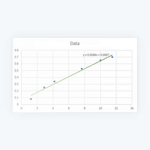
Best fit lines have many purposes and may help you significantly in visually representing your data.
Add a line of best fit trendline in Excel 2013 and up
In newer software versions, such as Excel 2019, the process of adding the best fit line to your charts is quite simple. The process requires you to create a chart first, and then add and customize the line to analyze your data correctly. This will create a line of best fit.
- Open the Excel document you want to add the best fit line to. Make sure there’s already data in the workbook.
- Highlight the data you want to analyze with the line of best fit. The selected data will be used to create a chart.

- Use the Ribbon interface and switch to the Insert tab. In the Charts panel, click on the Insert Scatter (X, Y) or Bubble Chart icon as shown on the image below.
- Select the first Scatter chart option, once again visible on the image below. This is going to insert a Scatter chart into your document, using the data you previously highlighted.
- Once the chart is inserted into your workbook, right-click on any of the data points. Select the Add Trendline option from the context menu.
- You should see a pane open on the right side of the window, called Format Trendline. Here, look for the Trendline Options tab, and then select Linear from the available options.
- At the bottom of the Trendline Options section, ensure that the checkbox next to Display Equation on Chart is enabled. This displays the math calculations used to create the best fit line. (Optional)
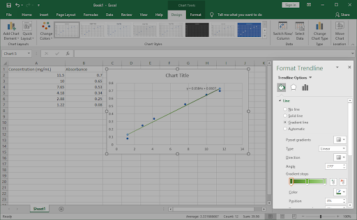
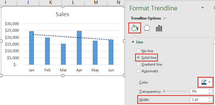
- To customize how the line of best fit appears on the chart, switch to the Fill & Line and Effects tabs in the Format Trendline pane. You can fully customize how the line looks, allowing you to easily differentiate it from the rest of your chart.

- Click the X in the top-right corner of the Format Trendline panel to exit it. You should be able to work with your line of best fit inserted into the chart.

Tip: When your chart is selected, customize the style and colors using the Design tab. You can create unique charts formatted just the way you want them. Combine this with the trendline customization options to fully personalize your charts.
Add a line of best fit trendline in Excel 2010 and older
For older Excel releases, such as Excel 2010 and below, the process is slightly different. Don’t worry — the steps below will guide you through making this chart line.
- Open the Excel document you want to add the best fit line to. Make sure there’s already data in the workbook.
- Highlight the data you want to analyze with the line of best fit. The selected data will be used to create a chart.
- Switch to the Insert tab. Click on Scatter in the charts category, and then select the first scatter chart on the list. (See image below)
- Select the newly created chart, and then switch to the Layout tab in the Chart Tools section. Here, expand the Trendline section and click on More Trendline Options.

- The Format Trendline window will pop up on the screen. First, select Polynomial from the Trend/Regression Type section. Next, ensure that the checkbox next to the Display Equation on chart is enabled.

- Click the Close button, and then check your chart. The line of best fit should appear visible now.


Final thoughts
If you need any further help with Excel, don’t hesitate to reach out to our customer service team, available 24/7 to assist you. Return to us for more informative articles all related to productivity and modern-day technology!
Would you like to receive promotions, deals, and discounts to get our products for the best price? Don’t forget to subscribe to our newsletter by entering your email address below! Receive the latest technology news in your inbox and be the first to read our tips to become more productive.
You may also like
» How to Split Column in Excel
» How To Add and Remove Leading Zeros in Excel
» 14 Excel Tricks That Will Impress Your Boss
A trendline, often called “the best-fit line,” is a line that shows the trend of the data. As you have seen in many charts, it shows the overall trend or pattern, or direction from the existing data points. Excel provides the option of plotting the trend line on the chart. When we add this trend line to the chart, it looks like a line chart without any ups and downs.
Table of contents
- Excel Trend Line
- How to Add and Insert Trend Line in Excel?
- How to Format the Trendline in Excel Chart?
- Things to Remember
- Recommended Articles
How to Add and Insert Trend Line in Excel?
You can download this Trend Line Excel Template here – Trend Line Excel Template
To add a trendline in Excel, we need to insert the chart for the available data. Before adding a trend line, remember the Excel charts supporting the trendline. For example, we can add a trendline to a column chart, line chart, bar chart, scattered chart or XY chart, stock chart, or In Excel, a bubble chart is a type of scatter plot that uses bubbles to display values and comparisons. Like scatter plots, bubble charts compare data on both horizontal and vertical axes.read more.
But we cannot add a trendline to 3-D or stacked charts, radar charts, Making a pie chart in excel can help you with the pictorial representation of your data and simplifies the analysis process. There are multiple kinds of pie chart options available on excel to serve the varying user needs.read more, and similar kinds of charts.
- The best example of plotting a trendline is monthly sales numbers. Below are the monthly sales numbers to create a chart.

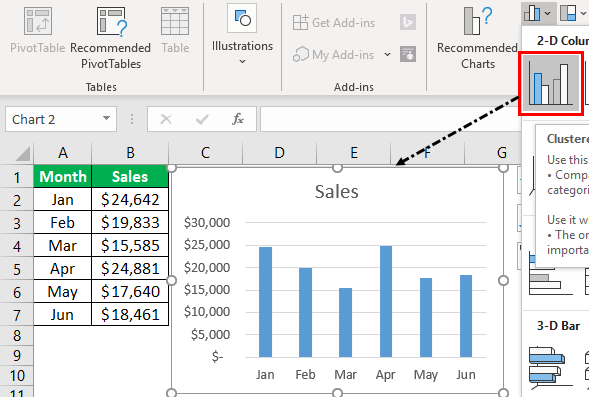
- To add a trendline, we need to create a column or line chart in Excel for the above data. Therefore, we will insert a column chart in Excel for this data.

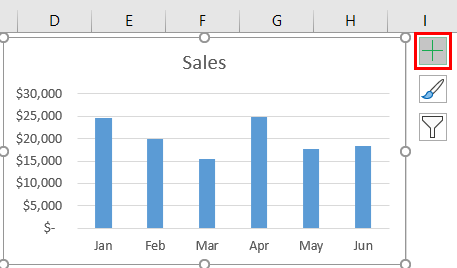
- Once the chart is inserted, adding the trend line is easy in Excel 2013 and the above versions. Select the chart. It will show the PLUS icon on the right side.

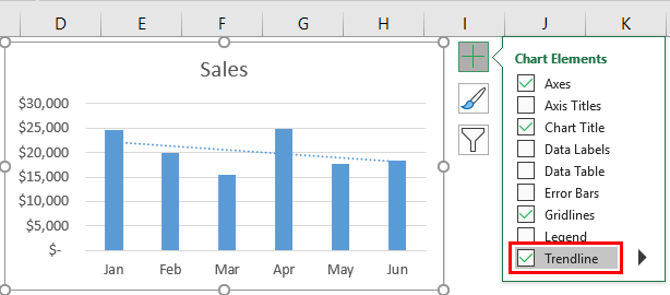
- Click on this PLUS icon to see various options related to this chart. For example, we can see the “Trendline” option at the end of the options. Click on this to add a trend line.

- So, our trendline is added to the chart. If you have inserted the LINE CHART in place of COLUMN CHART, all the steps are the same as inserting the trendline in Excel.
We can also add trend lines in multiple ways. Another way is to select column bars and right-click on the bars to see options. From the options, choose “ADD TRENDLINE.”


It will add the default trend line of “Linear Trend Line.” The best-fit trend line shows whether the data is trending upwards or downwards.
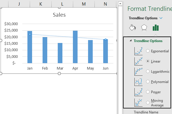
We have several trend line types, below are the types of the trend line.
- Exponential Trendline
- Linear Trendline
- Logarithmic Trendline
- Polynomial Trendline
- Power Trendline
- Moving Average Trendline
All these trendlines are part of the statistics. One of the other popular trendlines is the “Moving Average” trendline.
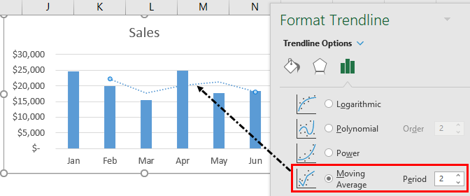
The “Moving Average” trendline shows the trend of the average of a specific number of periods. For example, the quarterly trend of the data. Right-click on column bars to apply the moving average trendline and choose “Add Trendline.” It will open the “Format Trendline” window to the right end of the worksheet.
In the above window, choose the “Moving Average” option and set the period to 2. It will add the trendline for the average of every 2 periods.
How to Format the Trendline in Excel Chart?
The default trendline does not have any special effects on the trend line. Therefore, we need to format the trend line to make it more appealing.
Select the trend line and press Ctrl +1. Then, in the “Format Trendline” window, choose “FILL” and “LINE,” make the width 2 pt, and the color dark blue.
This Excel trendline can also forecast the sales numbers for the next months. To do this, go to “Trendline Options, “Forecast,” and make “Forward” to 3 periods.
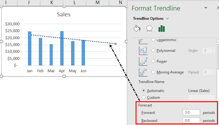
As shown in the above image, we have added a forward trend for 3 periods, increasing the trend line for 3 months.

From this chart, our trendline shows a continuous decline in sales numbers.
Things to Remember
- A trendline is a built-in tool in Excel.
- The “Moving Average” trendline shows the average trend line of the mentioned periods.
- We must always format the default trendline to make it more appealing.
Recommended Articles
This article has been a guide to TrendLine in Excel. Here, we learn how to add and insert the trendline in Excel, examples, and a downloadable Excel template. You may learn more about Excel from the following articles: –
- Excel Rotate Pie Chart
- Plots in Excel
- Grouped Bar Chart in Excel
- How to Make Dot Plots in Excel?
This article describes how to create the best fit graph for Microsoft Excel. The best-fitting straight line is the straight line used to show the trend pattern in the scatter plot. If you don’t know how to create this type of rule manually, you need to use a complex expression. Fortunately, Excel makes it easy to find accurate trend lines by doing some basic calculations.
With newer versions of software such as Excel 2019, the process of adding optimal rules to your graph is very straightforward. This process requires you to first create the graph and then add and adjust the rules to properly analyze the data. This will create the best line.
- Open the Excel document where you want to add the best rule.
- Make sure the workbook already has data. Mark the data you want to analyze with the best line.
- We need to Create a graph with the selected data.

- Go to the Insert tab using the Ribbon interface. Choose the Insert Scatter (X, Y) or Bubble Chart icon in the Charts window, as shown in the figure below.

- After clicking or selecting on the ‘Scatter with only Markers’ we are presented with a chart as a pop-up window where our data is scattered in a graph with Y and X axis representing 2nd column (frequency, in our example) and 1st column respectively.

- Right-click on any of the data points (on the chart) once the chart has been added into your worksheet and select Format option to open a context menu in right window pane.
- From the context menu, choose the Add Trendline option. (seen at the end of the menu)

- Upon that right side of the window, you should be seeing a pane labeled Format Trendline open (drop-down after adding trendline).
- Look for the Options tab and then choose Linear from the drop-down menu.

- Make sure the checkbox of Display Equation on Chart is enabled at the bottom of the Options section. The arithmetic calculations that were utilized to produce the best fit line are displayed now. (Optional)
- Move to the Fill & Line and Effects tabs in the Format window to modify how the line of best fit looks on the chart. You may completely modify the appearance of the line, making it stand out from the rest of your chart (here, color changed to black)

- Quit the format window by pressing close ‘X’ at the top and now you have your line of best fit put into the chart, you must be able to easily calculate and visualize.
Modify the design and colors of your chart using the Design tab once it has been selected. You may build custom charts that are formatted exactly as you want them. Merge this with the best fit line modification tools to make your charts really unique.
Add a line of best fit in Excel 2010 and before
The procedure differs somewhat from previous Excel versions, such as Excel 2010 and before.
But nothing to worry about, the instructions below will explain the process of creating this chart line.
- Open the Excel document to which the best fit line will be added. Check to see whether the worksheet already has data in it.
- With the line of best fit, highlight the data you wish to examine. A chart will be created using the selected data.
- Toggle over to the Insert tab. In the charts category, choose Scatter, and then the first scatter chart on the list. (See illustration below.)

- Switch to the Layout tab in the Chart Tools section after selecting the newly generated chart. Expand the Trendline section and select More Trendline Options from the drop-down menu.

5. On the Format Trendline window, go to the Trend/Regression Category section and pick Polynomial. After that, make sure the checkbox next to Display Equation on Chart is checked.

- Check your chart after clicking the Close button. The best-fit line should now be displayed.
Conclusion
That’s It for the tutorial. Here was a complete guide on how you can how to add a line of best fit in Excel in a newer version of excel as well as in the older. Hope you have learned well and are ready to implement in your worksheet.
Contents
- 1 How do you add a line of best fit in Excel 2016?
- 2 How do you make a line of best fit on Excel 2018?
- 3 How do you make a line of best fit?
- 4 What two things make a best fit line?
- 5 What is the best fit line on a graph?
- 6 Is line of best fit always straight?
- 7 When should you draw a line of best fit?
- 8 How do I find the slope of the line?
- 9 What is the equation of a line?
- 10 What is the slope between the points?
- 11 How do you find the slope of a line given two points?
- 12 What is a positive slope?
- 13 How do you find an equation given two points?
- 14 How do you find the equation of a line with one point?
- 15 How do you find the Y-intercept in an equation?
- 16 How do you write an equation of a line in slope intercept form?
- 17 How do you write an equation of a line from a graph?
- 18 What are the 3 slope formulas?
- 19 What is slope intercept form example?
- 20 What is standard form slope?
- 21 How do you interpret slope equations?
- 22 How do you interpret the slope of a best fit line?
- 23 How do you interpret the slope of a regression line?
How do you add a line of best fit in Excel 2016?
How to add Trendline in Excel
- STEP 1:Highlight your table of data, including the column headings:
- STEP 2: Select All Charts > Line > OK (Excel 2013 & 2016)
- STEP 3: Right-click on the line of your Line Chart and Select Add Trendline.
- STEP 4: Ensure Linear is selected and close the Format Trendline Window.
How do you make a line of best fit on Excel 2018?
Add a trendline
Select the + to the top right of the chart. Select Trendline. Note: Excel displays the Trendline option only if you select a chart that has more than one data series without selecting a data series. In the Add Trendline dialog box, select any data series options you want, and click OK.
How do you make a line of best fit?
How do I construct a best–fit line?
- Begin by plotting all your data.
- Draw a shape that encloses all of the data, (try to make it smooth and relatively even).
- Draw a line that divides the area that encloses the data in two even sized areas.
- Congratulations!
What two things make a best fit line?
A line of best fit is a straight line drawn through the maximum number of points on a scatter plot balancing about an equal number of points above and below the line.
What is the best fit line on a graph?
Line of best fit refers to a line through a scatter plot of data points that best expresses the relationship between those points.
Is line of best fit always straight?
About Lines of Best Fit
A line of best fit may be a straight line or a curve depending on how the points are arranged on the Scatter Graph.
When should you draw a line of best fit?
A line of best fit can only be drawn if there is strong positive or negative correlation. The line of best fit does not have to go through the origin. The line of best fit shows the trend, but it is only approximate and any readings taken from it will be estimations.
How do I find the slope of the line?
The slope of a line characterizes the direction of a line. To find the slope, you divide the difference of the y-coordinates of 2 points on a line by the difference of the x-coordinates of those same 2 points.
What is the equation of a line?
The equation of a line is typically written as y=mx+b where m is the slope and b is the y-intercept.
What is the slope between the points?
The slope between two points is calculated by finding the change in y-values and dividing by the change in x-values. For example, the slope between the points (7, -15) and (-8, 22) can be computed as follows: The difference in the y-values is -15-22 = -37.
How do you find the slope of a line given two points?
There are three steps in calculating the slope of a straight line when you are not given its equation.
- Step One: Identify two points on the line.
- Step Two: Select one to be (x1, y1) and the other to be (x2, y2).
- Step Three: Use the slope equation to calculate slope.
What is a positive slope?
A positive slope means that two variables are positively related—that is, when x increases, so does y, and when x decreases, y decreases also. Graphically, a positive slope means that as a line on the line graph moves from left to right, the line rises.
How do you find an equation given two points?
How do you find the equation of a line with one point?
Find the Equation of a Line Given That You Know a Point on the Line And Its Slope. The equation of a line is typically written as y=mx+b where m is the slope and b is the y-intercept. If you a point that a line passes through, and its slope, this page will show you how to find the equation of the line.
How do you find the Y-intercept in an equation?
To find the x-intercept of a given linear equation, plug in 0 for ‘y‘ and solve for ‘x’. To find the y–intercept, plug 0 in for ‘x’ and solve for ‘y‘.
How do you write an equation of a line in slope intercept form?
How do you write an equation of a line from a graph?
What are the 3 slope formulas?
There are three major forms of linear equations: point-slope form, standard form, and slope–intercept form. We review all three in this article.
What is slope intercept form example?
y = 5x + 3 is an example of the Slope Intercept Form and represents the equation of a line with a slope of 5 and and a y-intercept of 3. y = −2x + 6 represents the equation of a line with a slope of −2 and and a y-intercept of 6.
What is standard form slope?
Standard form is another way to write slope-intercept form (as opposed to y=mx+b). It is written as Ax+By=C. You can also change slope-intercept form to standard form like this: Y=-3/2x+3. A, B, C are integers (positive or negative whole numbers) No fractions nor decimals in standard form.
How do you interpret slope equations?
If the slope is given by an integer or decimal value we can always put it over the number 1. In this case, the line rises by the slope when it runs 1. “Runs 1” means that the x value increases by 1 unit. Therefore the slope represents how much the y value changes when the x value changes by 1 unit.
How do you interpret the slope of a best fit line?
The line’s slope equals the difference between points’ y-coordinates divided by the difference between their x-coordinates. Select any two points on the line of best fit. These points may or may not be actual scatter points on the graph. Subtract the first point’s y-coordinate from the second point’s y-coordinate.
How do you interpret the slope of a regression line?
The slope is interpreted as the change of y for a one unit increase in x. This is the same idea for the interpretation of the slope of the regression line. β ^ 1 represents the estimated increase in Y per unit increase in X. Note that the increase may be negative which is reflected when is negative.