
Updated 12/16/22: Stay up to date on the latest from Excel and download Excel templates today.
Excel provides you with different ways to calculate percentages. For example, you can use Excel to calculate the percentage of correct answers on a test, discount prices using various percent assumptions, or percent change between two values. Calculating a percentage in Excel is an easy two-step process. First, you format the cell to indicate the value is a percent, and then you build the percent formula in a cell.
Format values as percentages
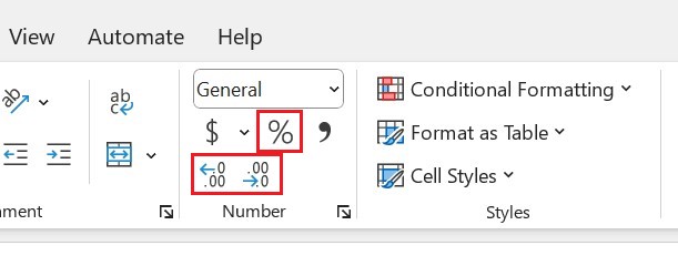
To show a number as a percent in Excel, you need to apply the Percentage format to the cells. Simply select the cells to format, and then click the Percent Style (%) button in the Number group on the ribbon’s Home tab. You can then increase (or decrease) the decimal place as needed. (See Rounding issues below for more information.)
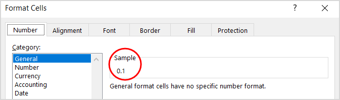
In Excel, the underlying value is always stored in decimal form. So, even if you’ve used number formatting to display something as a percentage (10%), that’s just what it is—formatting or a symbolic representation of the underlying value. Excel always performs calculations on that underlying value, which is a decimal (0.1). To double-check the underlying value, select the cell, press Ctrl + 1, and look in the Sample box on the General category.
Here are a few things to keep in mind when formatting percentages:
Format existing values—When you apply percentage formatting to a cell that already has a number in it, Excel multiplies that number by 100 and adds the % sign at the end. So for example, if you type 10 into cell A2 and then apply the percentage number format, Excel will multiply your number by 100 to show it as a percentage (remember that 1% is one part of one hundred), so you’ll see 1000% displayed in the cell, not 10%. To get around this, you can calculate your numbers as percentages first.
For example, if you type the formula =10/100 in cell A2, Excel will display the result as 0.1. If you then format that decimal as a percentage, the number will be displayed as 10%, as you‘d expect. You can also just type the number in its decimal form directly into the cell—that is, type 0.1 and then apply the percentage format.
Rounding issues—Sometimes what you see in a cell (for example 10%) doesn’t match the number you expected to see (such as 9.75%). To see the true percentage in the cell, rather than a rounded version, increase the decimal places. Again, Excel always uses the underlying value to perform calculations.
Format empty cells—Excel behaves differently when you pre-format empty cells with percentage formatting and then enter numbers. Numbers equal to and larger than 1 are converted to percentages by default; numbers smaller than 1 that are not preceded with a zero are multiplied by 100 to convert them to percentages. For example, if you type 10 or .1 in a preformatted cell, you’ll see 10% appear in the cell. Now, if you type 0.1 in the cell, Excel will return 0% or 0.10% depending on the decimal setting.
Format as you type—If you type 10% directly in the cell, Excel will automatically apply percentage formatting. This is useful when you want to type just a single percentage on your worksheet, such as a tax or commission rate.
Negative percentages—If you want negative percentages to be formatted differently—for example, to appear as red text or within parentheses—you can create a custom number format such as 0.00%;[Red]-0.00% or 0.00%_);(0.00%).

Get a better picture of your data.
Formulas to calculate percentages
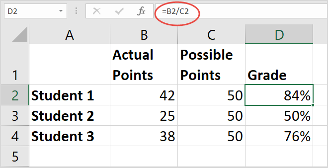
As with any formula in Excel, you need to start by typing an equal sign (=) in the cell where you want your result, followed by the rest of the formula. The basic formula for calculating a percentage is =part/total.
In the example below, Actual Points/Possible Points = Grade %:
Say you want to reduce a particular amount by 25%, like when you’re trying to apply a discount. Here, the formula will be =Price*1-Discount %. (Think of the “1” as a stand-in for 100%.)
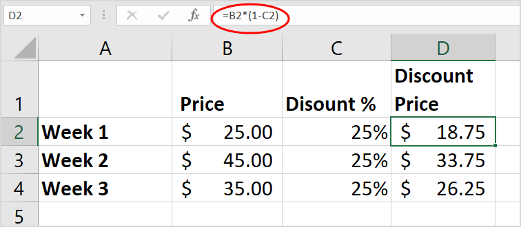
To increase the amount by 25%, simply replace the minus sign in the formula above with a plus sign.
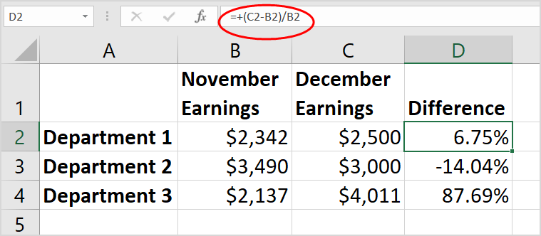
The next example is slightly more complicated. Say the earnings for your department are $2,342 in November and $2,500 in December and you want to find the percentage change in earnings between these two months. To find the answer, divide the difference between December and November’s earnings ($158) by the value of November’s earnings ($2,342).

Task management in Microsoft 365
Collaborate on shared Office documents, including Excel, Word, and PowerPoint.
Learn more
Start your free trial of Excel.
Learn more about how to format numbers as percentages and discover more examples of calculating percentages.
![]()
![]()
Share
- oneHOWTO
- Technology
- Software
- Microsoft Excel
- Exclel functions
- How to calculate a percentage in Excel


Microsoft Excel is a tool which allows you to calculate numeric and alphanumeric numbers through a calculation sheet. This data is shown in cells, which are usually distributed in a two-dimensional shape of columns and rows. In Excel, a cell is the base of information in a calculation sheet. You must use the cell to insert values and formulas to make several calculations, but today we want to show you how to calculate a percentage in Excel.
You’ll need:
- Microsoft Excel
Steps to follow:
1
Let’s set an example to calculate a percentage in Excel: if in an office of 50 people only 20 go up the stairs, what percentage of the people in the office go up the stairs?
To get this percentage on Excel, you must select a cell, for example: D5.

2
This way, you’ll apply a rule of three:
50 — 100%
20 — x
That is to say, if 50 people are 100%, what percentage are 20?
To calculate this mathematical operation on Excel and find the percentage, you have to write «=(20/50)*100» (without the commas) on the selected cell.

3
Press Enter and you’ll see how Excel gives you your desired percentage, in our case: 40. This way, we can say that if there are 50 people in the office and 20 use the stairs, 40% of the workers use the stairs instead of the lift.

4
Another way of calculating a percentage on Excel is using previously introduced values on the calculation sheet. Following the example, we’ll write the values the exercise gives us as if we were doing a rule of three.
Select a new empty cell, in this case D5, and write the «equal» symbol: =

5
Next, you need to select the cells that have numeric values and write the mathematical symbols of the needed operations and finally press Intro or Enter. In this way, the formula will be done with alphanumeric codes in the cells, in our case: «=A3/A2*B2»
You should know these symbols on Excel:
- + add up
- — subtract
- * multiply
- / divide

If you want to read similar articles to How to calculate a percentage in Excel, we recommend you visit our Software category.
Write a comment
How to calculate a percentage in Excel
How to calculate a percentage in Excel
- oneHOWTO
- Technology
- Software
- Microsoft Excel
- Exclel functions
- How to calculate a percentage in Excel
Back to top
Skip to content
В этом руководстве вы познакомитесь с быстрым способом расчета процентов в Excel, найдете базовую формулу процента и еще несколько формул для расчета процентного изменения, процента от общей суммы и т.д.
Расчет процента нужен во многих ситуациях, будь то комиссия продавца, ваш подоходный налог или процентная ставка по кредиту. Допустим, вам посчастливилось получить скидку 25% на новый телевизор. Это хорошая сделка? И сколько в итоге придется заплатить?
Сейчас мы рассмотрим несколько методов, которые помогут вам эффективно вычислять процент в Excel, а также освоим основные формулы процента, которые избавят вас от догадок при расчетах.
- Базовая формула подсчета процента от числа.
- Как посчитать процент между числами по колонкам.
- Как рассчитать процент по строкам.
- Доля в процентах.
- Считаем процент скидки
- Отклонение в процентах для отрицательных чисел
- Вычитание процентов
- Как избежать ошибки деления на ноль
Что такое процент?
Как вы, наверное, помните из школьного урока математики, процент — это доля от 100, которая вычисляется путем деления двух чисел и умножения результата на 100.
Основная процентная формула выглядит следующим образом:
(Часть / Целое) * 100% = Процент
Например, если у вас было 20 яблок и вы подарили 5 своим друзьям, сколько вы дали в процентном отношении? Проведя несложный подсчет =5/20*100% , вы получите ответ — 25%.
Так обычно рассчитывают проценты в школе и в повседневной жизни. Вычислить процентное соотношение в Microsoft Excel еще проще, поскольку он выполняет некоторые операции за вас автоматически.
К сожалению, универсальной формулы расчета процентов в Excel, которая охватывала бы все возможные случаи, не существует. Если вы спросите кого-нибудь: «Какую формулу процентов вы используете, чтобы получить желаемый результат?», Скорее всего, вы получите ответ типа: «Это зависит от того, какой именно результат вы хотите получить».
Итак, позвольте мне показать вам несколько простых формул для расчета процентов в Excel.
Расчет процентов в Excel.
Основная формула для расчета процента от числа в Excel такая же, как и во всех сферах жизни:
Часть / Целое = Процент
Если вы сравните ее с основной математической формулой для процента, которую мы указали чуть выше, то заметите, что в формуле процента в Excel отсутствует часть * 100. При вычислении процента в Excel вам совершенно не обязательно умножать полученную дробь на 100, поскольку программа делает это автоматически, когда процентный формат применяется к ячейке.
И если в Экселе вы будете вводить формулу с процентами, то можно не переводить в уме проценты в десятичные дроби и не делить величину процента на 100. Просто укажите число со знаком %.
То есть, чтобы, к примеру, посчитать 10% в Экселе, то вместо =A1*0,1 или =A1*10/100, просто запишите формулу процентов =A1*10%.
Хотя с точки зрения математики все 3 варианта возможны и все они дадут верный результат.
А теперь давайте посмотрим, как можно использовать формулу процента в Excel для реальных данных. Предположим, в вашей таблице Эксель записана сумма заказанных товаров в столбце F и оставленных товаров в столбце G. Чтобы высчитать процент доставленных товаров, выполните следующие действия:
- Введите формулу =G2/F2 в ячейку H2 и скопируйте ее на столько строк вниз, сколько вам нужно.
- Нажмите кнопку «Процентный стиль» ( меню «Главная» > группа «Число»), чтобы отобразить полученные десятичные дроби в виде процентов.
- Не забудьте при необходимости увеличить количество десятичных знаков в полученном результате.
- Готово!


Такая же последовательность шагов должна быть выполнена при использовании любой другой формулы процентов в Excel.
На скриншоте ниже вы видите округленный процент доставленных товаров без десятичных знаков.
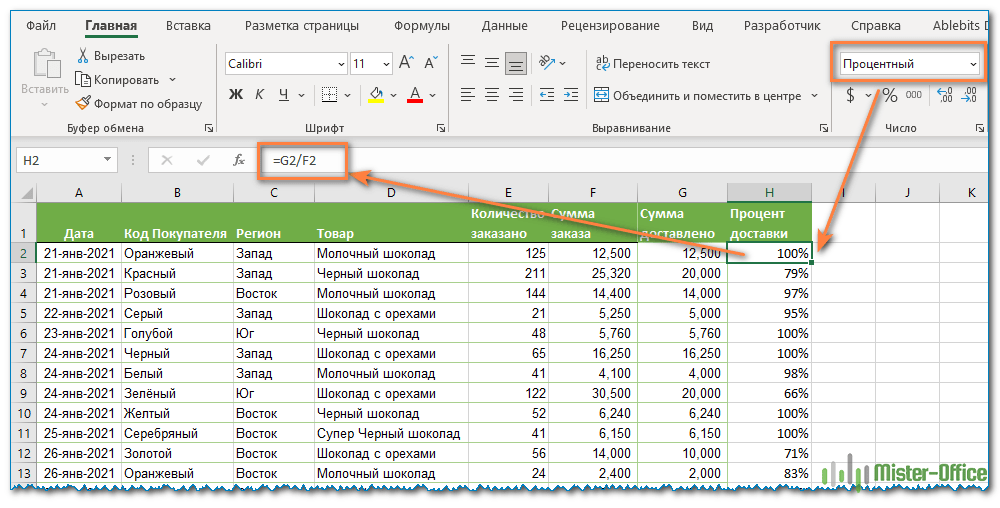
Чтобы определить процент доставки, мы сумму доставленных товаров делим на сумму заказов. И используем в ячейке процентный формат, при необходимости показываем десятичные знаки.
Запишите формулу в самую верхнюю ячейку столбца с расчетами, а затем протащите маркер автозаполнения вниз по столбцу. Таким образом, мы посчитали процент во всём столбце.
Как найти процент между числами из двух колонок?
Предположим, у нас имеются данные о продажах шоколада за 2 месяца. Необходимо определить, какие произошли изменения в реализации. Проще и нагляднее всего отклонения в продажах выразить в процентах.
Чтобы вычислить разницу в процентах между значениями A и B, используйте следующую формулу:
Процентное изменение = (B — A) / A
При применении этой формулы к реальным данным важно правильно определить, какое значение равно A, а какое — B. Например, вчера у вас было 80 яблок, а сейчас — 100. Это означает, что теперь у вас на 20 яблок больше, чем раньше, что произошло увеличение на 25%. Если у вас было 100 яблок, а теперь – 90, то количество яблок у вас уменьшилось на 10, то есть на 10%.
Учитывая вышеизложенное, наша формула Excel для процентного изменения принимает следующую форму:
=(новое_значение – старое_значение)/старое_значение
А теперь давайте посмотрим, как вы можете использовать эту формулу процентного изменения в своих таблицах.
В нашем случае —
=(E2-D2)/D2
Эта формула процентного изменения вычисляет процентное увеличение (либо уменьшение) в феврале (столбец E) по сравнению с январём (столбец В).
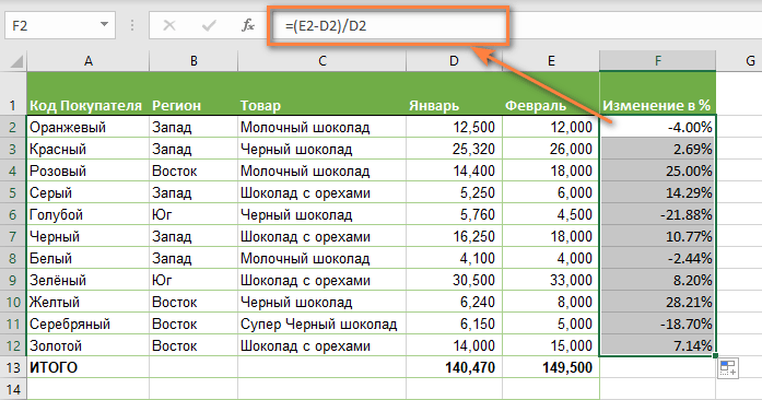
И затем при помощи маркера заполнения копируем ее вниз по столбцу. Не забудьте применить процентный формат.
Отрицательные проценты, естественно, означают снижение продаж, а положительные — их рост.
Аналогичным образом можно подсчитать и процент изменения цен за какой-то период времени.
Как найти процент между числами из двух строк?
Такой расчет применяется? Если у нас есть много данных об изменении какого-то показателя. И мы хотим проследить, как с течением времени изменялась его величина. Поясним на примере.
Предположим, у нас есть данные о продажах шоколада за 12 месяцев. Нужно проследить, как изменялась реализация от месяца к месяцу. Цифры в столбце С показывают, на сколько процентов в большую или меньшую сторону изменялись продажи в текущем месяце по сравнению с предшествующим.

Обратите внимание, что первую ячейку С2 оставляем пустой, поскольку январь просто не с чем сравнивать.
В С3 записываем формулу:
=(B3-B2)/B2
Можно также использовать и другой вариант:
=B3/B2 — 1
Копируем содержимое этой ячейки вниз по столбцу до конца таблицы.
Если нам нужно сравнивать продажи каждого месяца не с предшествующим, а с каким-то базисным периодом (например, с январём текущего года), то немного изменим нашу формулу, использовав абсолютную ссылку на цифру продаж января:
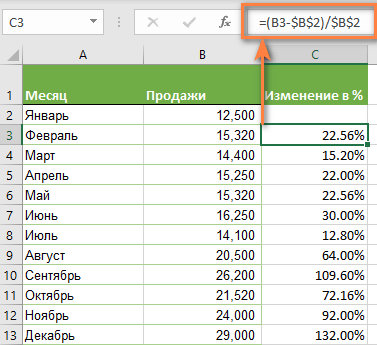
Абсолютная ссылка на $B$2 останется неизменной при копировании формулы в C4 и ниже:
=(B3-$B$2)/$B$2
А ссылка на B3 будет изменяться на B4, B5 и т.д.
Напомню, что по умолчанию результаты отображаются в виде десятичных чисел. Чтобы отобразить проценты , примените к столбцу процентный формат. Для этого нажмите соответствующую кнопку на ленте меню или используйте комбинацию клавиш Ctrl + Shift + %.
Десятичное число автоматически отображается в процентах, поэтому вам не нужно умножать его на 100.
Расчет доли в процентах (удельного веса).
Давайте рассмотрим несколько примеров, которые помогут вам быстро вычислить долю в процентах от общей суммы в Excel для различных наборов данных.
Пример 1. Сумма находится в конце таблицы в определенной ячейке.
Очень распространенный сценарий — это когда у вас есть итог в одной ячейке в конце таблицы. В этом случае формула будет аналогична той, которую мы только что обсудили. С той лишь разницей, что ссылка на ячейку в знаменателе является абсолютной ссылкой (со знаком $). Знак доллара фиксирует ссылку на итоговую ячейку, чтобы она не менялась при копировании формулы по столбцу.
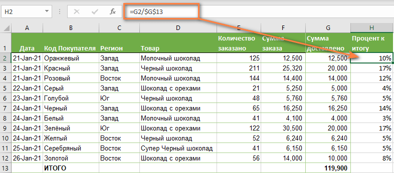
Возьмем данные о продажах шоколада и рассчитаем долю (процент) каждого покупателя в общем итоге продаж. Мы можем использовать следующую формулу для вычисления процентов от общей суммы:
=G2/$G$13
Вы используете относительную ссылку на ячейку для ячейки G2, потому что хотите, чтобы она изменилась при копировании формулы в другие ячейки столбца G. Но вы вводите $G$13 как абсолютную ссылку, потому что вы хотите оставить знаменатель фиксированным на G13, когда будете копировать формулу до строки 12.
Совет. Чтобы сделать знаменатель абсолютной ссылкой, либо введите знак доллара ($) вручную, либо щелкните ссылку на ячейку в строке формул и нажмите F4.
На скриншоте ниже показаны результаты, возвращаемые формулой. Столбец «Процент к итогу» отформатирован с применением процентного формата.
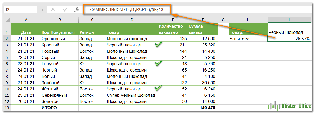
Пример 2. Часть итоговой суммы находится в нескольких строках.
В приведенном выше примере предположим, что у вас в таблице есть несколько записей для одного и того же товара, и вы хотите знать, какая часть общей суммы приходится на все заказы этого конкретного товара.
В этом случае вы можете использовать функцию СУММЕСЛИ, чтобы сначала сложить все числа, относящиеся к данному товару, а затем разделить это число на общую сумму заказов:
=СУММЕСЛИ( диапазон; критерий; диапазон_суммирования ) / Итог
Учитывая, что столбец D содержит все наименования товаров, столбец F перечисляет соответствующие суммы, ячейка I1 содержит наименование, которое нас интересует, а общая сумма находится в ячейке F13, ваш расчет может выглядеть примерно так:
=СУММЕСЛИ(D2:D12;I1;F2:F12)/$F$13
Естественно, вы можете указать название товара прямо в формуле, например:
=СУММЕСЛИ(D2:D12;”Черный шоколад”;F2:F12)/$F$13
Но это не совсем правильно, поскольку эту формулу придется часто корректировать. А это затратно по времени и чревато ошибками.
Если вы хотите узнать, какую часть общей суммы составляют несколько различных товаров, сложите результаты, возвращаемые несколькими функциями СУММЕСЛИ, а затем разделите это число на итоговую сумму. Например, по следующей формуле рассчитывается доля черного и супер черного шоколада:
=(СУММЕСЛИ(D2:D12;”Черный шоколад”;F2:F12)/$F$13 + =СУММЕСЛИ(D2:D12;”Супер черный шоколад”;F2:F12)) / $F$13
Естественно, текстовые наименования товаров лучше заменить ссылками на соответствующие ячейки.
Для получения дополнительной информации о функции суммирования по условию ознакомьтесь со следующими руководствами:
- Как использовать функцию СУММЕСЛИ в Excel
- СУММЕСЛИМН и СУММЕСЛИ в Excel с несколькими критериями
Процент скидки
Формулы процентов пригодятся для расчета уровня скидки. Итак, отправляясь за покупками, помните следующее:
Скидка в % = (цена со скидкой – обычная цена) / обычная цена
Скидка в % = цена со скидкой / обычная цена — 1
В результатах вычисления процент скидки отображается как отрицательное значение, поскольку новая цена со скидкой меньше старой обычной цены. Чтобы вывести результат в виде положительного числа , оберните формулы в функцию ABS. Например:
=ABS((C2-B2)/B2)
или
=ABS((C2/B2 — 1)
Так будет гораздо привычнее.

Как рассчитать отклонение в процентах для отрицательных чисел
Если некоторые из исходных значений представлены отрицательными числами, приведенные выше формулы не будут работать.
Обычный обходной путь — сделать знаменатель в формуле положительным числом. Для этого воспользуйтесь функцией ABS:
( Новое_значение – старое_значение ) / ABS( старое_значение )
Со старым значением в B2 и новым значением в C2 формула выглядит следующим образом:
=(C2-B2)/ABS(B2)
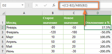
Как видите, достаточно корректно работает с самыми разными комбинациями положительных и отрицательных чисел.
Положительный процент означает рост, отрицательный — снижение величины показателя.
Вычитание процентов.
Часто случается, что вам известен процент скидки на товар. И вам нужно высчитать, какой процент от первоначальной стоимости придётся заплатить. Как мы уже говорили, процент в Экселе — это обычное число. Поэтому и правила вычисления здесь – как с обычными числами.

Формула расчета в Excel будет выглядеть так:
=1 – процент_скидки
Как обычно, не забываем про процентный формат ячеек.
Предотвратить ошибки деления на ноль #ДЕЛ/0
Если вы хотите посчитать процент от числа в таблице, и ваш набор данных содержит несколько нулевых значений, заключите формулы в функцию ЕСЛИОШИБКА, чтобы предотвратить появление ошибок деления на ноль (#ДЕЛ/0! или #DIV/0!).
=IFERROR(=ЕСЛИОШИБКА((C2-B2)/B2;0)
=IFERROR(=ЕСЛИОШИБКА(C2/B2-1;0)

Вот как можно вычислить процент от числа в Excel. И даже если работа с процентами никогда не была вашим любимым видом математики, с помощью этих основных процентных формул вы можете заставить Excel делать работу за вас.
На сегодня все, спасибо, что прочитали!
To change numbers to a percentage in Excel using the Ribbon, click on the Ribbon, make sure you are on the home Ribbon tab.
Converting Numbers to Percentage in Excel
- Highlight the desired cells.
- Right click them.
- Click the Format Cells option.
- Click the Number category.
- Then chose the percentage tab.
Contents
- 1 How do I convert a number into a percentage?
- 2 How do I convert a number to a percentage in Excel without multiplying by 100?
- 3 How do you turn 0.65 into a percent?
- 4 What is .08 as a percent?
- 5 How do I show a percentage without the symbol in Excel?
- 6 How do I get Excel to automatically add percentages?
- 7 How do you convert 3.1 to a percent?
- 8 How do you write 12.35 as a percent?
- 9 How do you turn 4.5 into a percent?
- 10 What is 0.12 as a percent?
- 11 What is 1.3 as a percent?
- 12 What is 0.8 as a number?
- 13 What is the formula to remove percentage in Excel?
- 14 How do I add 10 percent in Excel?
- 15 What is a percentage formula?
- 16 How do you write 7 4 as a percent?
- 17 What is the 20% as a fraction?
- 18 What is the process for converting a fraction to a decimal?
- 19 What fraction is equivalent to 25 percent?
- 20 What is the percentage of 3 8?
How do I convert a number into a percentage?
Multiply by 100 to convert a number from decimal to percent then add a percent sign %.
- Converting from a decimal to a percentage is done by multiplying the decimal value by 100 and adding %.
- Example: 0.10 becomes 0.10 x 100 = 10%
- Example: 0.675 becomes 0.675 x 100 = 67.5%
How do I convert a number to a percentage in Excel without multiplying by 100?
#1 select those numbers in new column, and then right click on it, and select Format Cells from the popup menu list. And the Format Cells dialog will open. #2 click Custom under Category list box, and type in “0%” in Type text box, and then click OK button.
How do you turn 0.65 into a percent?
Express 0.65 as a percent
- Multiply both numerator and denominator by 100. 0.65 × 100100.
- = (0.65 × 100) × 1100 = 65100.
- Write in percentage notation: 65%
What is .08 as a percent?
Decimal to percent conversion table
| Decimal | Percent |
|---|---|
| 0.07 | 7% |
| 0.08 | 8% |
| 0.09 | 9% |
| 0.1 | 10% |
How do I show a percentage without the symbol in Excel?
Enter the custom format as follows:
- Enter 0.00.
- While holding down Alt, enter 0010. This will put in a line break.
- Put in the %.
- Hit OK.
How do I get Excel to automatically add percentages?
Adding Percentages Using Excel
- Open Microsoft Excel.
- Enter the percentage you wish to add in cell B1 and include the percent sign, which automatically formats the number as a percentage.
- List the values to which you wish to add a percentage in column A, beginning at cell A2.
How do you convert 3.1 to a percent?
Express 3.1 as a percent
- Multiply both numerator and denominator by 100. 3.1 × 100100.
- = (3.1 × 100) × 1100 = 310100.
- Write in percentage notation: 310%
How do you write 12.35 as a percent?
It’s percentage is 1235 .
How do you turn 4.5 into a percent?
Decimal to Percentage (%) CalculatorTo convert from decimal to percent, just multiply the decimal value by 100. In this example we have: 4.5 × 100 = 450% (answer).
What is 0.12 as a percent?
Make use of the Free Decimal to Percent Calculator to change decimal value 0.12 to its equivalent percent value 0.0012% in no time along with the detailed steps.
What is 1.3 as a percent?
130%
1310 , 1310 , or 130% .
What is 0.8 as a number?
The decimal 0.8 is a rational number. It is equivalent to the fraction 8/10.
What is the formula to remove percentage in Excel?
Tip: You can also multiply the column to subtract a percentage. To subtract 15%, add a negative sign in front of the percentage, and subtract the percentage from 1, using the formula =1-n%, in which n is the percentage. To subtract 15%, use =1-15% as the formula.
How do I add 10 percent in Excel?
To increase a number by a percentage amount, multiply the original amount by 1+ the percent of increase. In the example shown, Product A is getting a 10 percent increase. So you first add 1 to the 10 percent, which gives you 110 percent. You then multiply the original price of 100 by 110 percent.
What is a percentage formula?
Percentage Formula
To determine the percentage, we have to divide the value by the total value and then multiply the resultant to 100. Percentage formula = (Value/Total value)×100. Example: 2/5 × 100 = 0.4 × 100 = 40 per cent.
How do you write 7 4 as a percent?
Divide 7 by 4 . Therefore, the fraction 74 is equivalent to 175% .
What is the 20% as a fraction?
Example Values
| Percent | Decimal | Fraction |
|---|---|---|
| 5% | 0.05 | 1/20 |
| 10% | 0.1 | 1/10 |
| 12½% | 0.125 | 1/8 |
| 20% | 0.2 | 1/5 |
What is the process for converting a fraction to a decimal?
The line in a fraction that separates the numerator and denominator can be rewritten using the division symbol. So, to convert a fraction to a decimal, divide the numerator by the denominator. If required, you can use a calculator to do this. This will give us our answer as a decimal.
What fraction is equivalent to 25 percent?
1/4
Answer: 25% as a fraction is 1/4.
What is the percentage of 3 8?
37.5%
To convert to percentage
To convert the fraction to decimal first convert to decimal and then multiply by 100. Therefore, the solution is 37.5%.

If you’re struggling with calculating percentage increases or decreases in Microsoft Excel, this guide will talk you through the process.
Microsoft Excel is great for basic and complicated calculations alike, including percentage differences. If you’re struggling to calculate percentage increases or decreases on paper, Excel can do it for you.
If you remember your school math, the process for calculating percentages in Excel is pretty similar. Here’s how to use Excel to calculate percentage increases and decreases. And perform other percentage calculations like percentages of a number.
Calculating Percentage Increase in Excel
Percentage increases involve two numbers. The basic mathematical approach for calculating a percentage increase is subtracting the second number from the first number. Using the sum of this figure, divide this remaining figure by the original number.
To give you an example, the cost of a household bill costs $100 in September, but $125 in October. To calculate this difference, you could use the excel formula =SUM(NEW-OLD)/OLD or, for this example, =SUM(125-100)/100 in Excel.
If your figures are in separate cells, you can replace numbers for cell references in your formula. For example, if September’s bill amount is in cell B4 and October’s bill amount is in cell B5, your alternative Excel formula would be =SUM(B5-B4)/B4.

The percentage increase between September and October is 25%, with this figure shown as a decimal number (0.25) by default in Excel using the formula above.
If you want to display this figure as a percentage in Excel, you’ll need to replace the formatting for your cell. Select your cell, then click the Percentage Style button in the Home tab, under the Number category.

You can also right-click your cell, click Format Cells, then select Percentages from the Category > Number menu to achieve the same effect.
Calculating Percentage Decrease in Excel
To calculate the percentage decrease between two numbers, you’ll use an identical calculation to the percentage increase. You subtract the second number from the first, then divide it by the first number. The only difference is that the first number will be smaller than the second number.
Continuing the above example, if a household bill is $125 in October, but it returns to $100 in November, you would use the excel formula =SUM(NEW-OLD)/OLD or, in this example, =SUM(100-125)/125.
Using cell references, if October’s bill amount of $125 is in cell B4 and November’s bill amount of $100 is in cell B5, your Excel formula for a percentage decrease would be =SUM(B5-B4)/B4.

The difference between October and November’s figures is 20%. Excel displays this as a negative decimal number (-0.2) in cells B7 and B8 above.
Setting the cell number type to Percentages using the Home > Percentage Styles button will change the decimal figure (-0.2) to a percentage (-20%).

Calculating a Percentage as a Proportion of a Number
Excel can also help you calculate a percentage as a proportion. This is the difference between one number, as your complete figure, and a smaller number. This requires an even simpler mathematical calculation than a percentage change.
To give you an example, if you have a debt of $100, and you’ve already paid $50, then the proportion of the debt you’ve paid (and coincidentally still owe) is 50%. To calculate this, you divide 50 by 100.
In Excel, the formula to calculate this example would be =50/100. Using cell references, where $100 is in cell B3 and $50 is in cell B4, the excel formula required is =B4/B3.

This uses only a basic division operator to give you the decimal number (0.5).
Converting this cell number type to Percentages by clicking Home > Percentage Style button will show the correct percentage figure of 50%.

How to Calculate Percentages of a Number
Calculating the percentage of a number is something that you’ll encounter in day-to-day life. A good example would be an item for sale, where a discount of 20% is being applied to the original price of $200. A store employee would need to know what 20% of $200 was. They could then subtract this number from the original price to provide the discounted price.
This requires another simple mathematical calculation in Excel. Only the multiplication operator (*) and percentage sign (%) are used here. To calculate what 20% of the original $200 price is, you can use either =20%*200 or =0.2*200 to calculate in Excel.
To use cell references, where 20% is in cell B4 and the original price of $200 is in cell B5, you could use the formula =B4*B5 instead.

The result is the same, whether you use 20%, 0.2, or separate cell references in your formula. 20% of $200 equals $40, as shown in cells B6 to B8 above.
Using Excel for Complex Calculations
As this guide shows, Excel is great for simple calculations, but it handles more complex ones, too. Calculations using functions like the VLOOKUP function are made easy, thanks to the built-in function search tool.
If you’re new to Excel, take advantage of some Excel tips every user should know to improve your productivity further.
![]()