Excel for Microsoft 365 Excel for Microsoft 365 for Mac Excel for the web Excel 2021 Excel 2021 for Mac Excel 2019 Excel 2019 for Mac More…Less
The IFS function checks whether one or more conditions are met, and returns a value that corresponds to the first TRUE condition. IFS can take the place of multiple nested IF statements, and is much easier to read with multiple conditions.
Simple syntax
Generally, the syntax for the IFS function is:
=IFS([Something is True1, Value if True1,Something is True2,Value if True2,Something is True3,Value if True3)
Please note that the IFS function allows you to test up to 127 different conditions. However, we don’t recommend nesting too many conditions with IF or IFS statements. This is because multiple conditions need to be entered in the correct order, and can be very difficult to build, test and update.
Syntax
-
IFS(logical_test1, value_if_true1, [logical_test2, value_if_true2], [logical_test3, value_if_true3],…)
|
Argument |
Description |
|
logical_test1 (required) |
Condition that evaluates to TRUE or FALSE. |
|
value_if_true1 (required) |
Result to be returned if logical_test1 evaluates to TRUE. Can be empty. |
|
logical_test2…logical_test127 (optional) |
Condition that evaluates to TRUE or FALSE. |
|
value_if_true2…value_if_true127 (optional) |
Result to be returned if logical_testN evaluates to TRUE. Each value_if_trueN corresponds with a condition logical_testN. Can be empty. |
Example 1
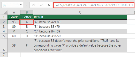
The formula for cells A2:A6 is:
-
=IFS(A2>89,»A»,A2>79,»B»,A2>69,»C»,A2>59,»D»,TRUE,»F»)
Which says IF(A2 is Greater Than 89, then return a «A», IF A2 is Greater Than 79, then return a «B», and so on and for all other values less than 59, return an «F»).
Example 2
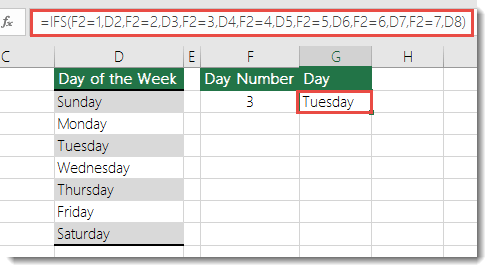
The formula in cell G7 is:
-
=IFS(F2=1,D2,F2=2,D3,F2=3,D4,F2=4,D5,F2=5,D6,F2=6,D7,F2=7,D8)
Which says IF(the value in cell F2 equals 1, then return the value in cell D2, IF the value in cell F2 equals 2, then return the value in cell D3, and so on, finally ending with the value in cell D8 if none of the other conditions are met).
Remarks
-
To specify a default result, enter TRUE for your final logical_test argument. If none of the other conditions are met, the corresponding value will be returned. In Example 1, rows 6 and 7 (with the 58 grade) demonstrate this.
-
If a logical_test argument is supplied without a corresponding value_if_true, this function shows a «You’ve entered too few arguments for this function» error message.
-
If a logical_test argument is evaluated and resolves to a value other than TRUE or FALSE, this function returns a #VALUE! error.
-
If no TRUE conditions are found, this function returns #N/A error.
Need more help?
You can always ask an expert in the Excel Tech Community or get support in the Answers community.
Related Topics
IF function
Advanced IF functions — Working with nested formulas and avoiding pitfalls
Training videos: Advanced IF functions
The COUNTIF function will count values based on a single criteria
The COUNTIFS function will count values based on multiple criteria
The SUMIF function will sum values based on a single criteria
The SUMIFS function will sum values based on multiple criteria
AND function
OR function
VLOOKUP function
Overview of formulas in Excel
How to avoid broken formulas
Detect errors in formulas
Logical functions
Excel functions (alphabetical)
Excel functions (by category)
Need more help?
The IFs function evaluates multiple expressions and returns a result that corresponds to the first TRUE result. You can use the IFS function when you want a self-contained formula to test multiple conditions at the same time without nesting multiple IF statements. Formulas based on IFS are shorter and easier to read and write.
Conditions are provided to the IFS function as test/value pairs, and IFS can handle up to 127 conditions. Each test represents a logical test that returns TRUE or FALSE, and the value that follows will be returned when the test returns TRUE. In the event that more than one condition returns TRUE, the value corresponding to the first TRUE result is returned. For this reason, it is important to consider the order in which conditions appear.
Structure
An IFS formula with 3 tests can be visualized like this:
=IFS(
test1,value1 // pair 1
test2,value2 // pair 2
test3,value3 // pair 3
)
A value is returned by IFS only when the previous test returns TRUE, and the first test to return TRUE «wins». For better readability, you can add line breaks to an IFS formula as shown above.
Note: the IFS function does not provide an argument for a default value. See Example #3 below for a workaround.
Example #1 — grades, lowest to highest
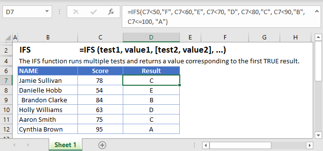
In the example shown below, the IFS function is used to assign a grade based on a score. The formula in E5, copied down, is:
=IFS(C5<60,"F",C5<70,"D",C5<80,"C",C5<90,"B",C5>=90,"A")
Notice the conditions are entered «in order» to test lower scores first. The grade associated with the first test to return TRUE is returned.
Example #2 — rating, highest to lowest
In a simple rating system, a score of 3 or greater is «Good», a score between 2 and 3 is «Average», and anything below 2 is «Poor». To assign these values with IFS, three conditions are used:
=IFS(A1>=3,"Good",A1>=2,"Average",A1<2,"Poor")
Notice in this case conditions are arranged to test higher values first.
Example #3 — default value
The IFS function does not have a built-in default value to use when all conditions are FALSE. However, to provide a default value, you can enter TRUE as a final test, followed by a value to use as a default.
In the example below, a status code of 100 is «OK», a code of 200 is «Warning», and a code of 300 is «Error». Any other code value is invalid, so TRUE is provided as the final test, and «Invalid» is provided as a «default» value.
=IFS(A1=100,"OK",A1=200,"Warning",A1=300,"Error",TRUE,"Invalid")
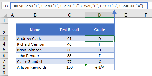
When the value in A1 is 100, 200, or 300, IFS will return the messages shown above. When A1 contains any other value (including when A1 is empty) IFS will return «Invalid». Without this final condition, IFS will return #N/A when a code is not recognized.
Note: IFS is a new function available in Excel 365 and Excel 2019.
IFS versus SWITCH
Like the SWITCH function, the IFS function allows you to test more than one condition in a single self-contained formula. Both functions make it easier to write (and read) a formula with many conditions. One advantage of SWITCH over IFS is that the expression appears just once in the function and does not need to be repeated. In addition, SWITCH can accept a default value. However, SWITCH is limited to exact matching. It is not possible to use operators like greater than (>) or less than (<) with the standard syntax. In contrast, the IFS function requires expressions for each condition, so you can use logical operators as needed.
Notes
- The IFS function does not have a built-in default value to use when all conditions are FALSE.
- To provide a default value, enter TRUE as a final test, and a value to return when no other conditions are met.
- All logical tests must return TRUE or FALSE. Any other result will cause IFS to return a #VALUE! error.
- If no logical tests return TRUE, IFS will return the #N/A error.
This Excel tutorial explains how to use the Excel IFS function with syntax and examples.
Description
The Microsoft Excel IFS function lets you specify multiple IF conditions within one function call.
The IFS function is a built-in function in Excel that is categorized as a Logical Function. It can be used as a worksheet function (WS) in Excel. As a worksheet function, the IFS function can be entered as part of a formula in a cell of a worksheet.
This function replaces the old method of nesting multiple IF functions and lets you enter up to 127 conditions making your formulas easy to read and understand. The only downside to this function is that you can’t specify an ELSE condition, but we do have a workaround which we will show you later in the tutorial.
Subscribe
If you want to follow along with this tutorial, download the example spreadsheet.
Download Example
Syntax
The syntax for the IFS function in Microsoft Excel is:
IFS( condition1, return1 [,condition2, return2] ... [,condition127, return127] )
Parameters or Arguments
- condition1, condition2, … condition127
- The condition that you want to test. There can be up to 127 conditions entered.
- return1, return2, … return127
- The value that is returned if the corresponding condition is TRUE. All conditions are evaluated in the order that they are listed so once the function finds a condition that evaluates to TRUE, the IFS function will return the corresponding value and stop processing any further conditions.
Returns
The IFS function returns any datatype such as a string, numeric, date, etc.
If none of the conditions evaluate to TRUE, the IFS function will return the #N/A error.
Applies To
- Excel for Office 365, Excel 2019
Type of Function
- Worksheet function (WS)
Example (as Worksheet Function)
Let’s explore how to use the IFS function as a worksheet function in Microsoft Excel.
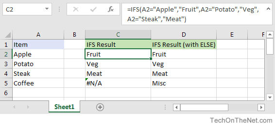
Based on the Excel spreadsheet above, the following IFS examples would return:
=IFS(A2="Apple","Fruit",A2="Potato","Veg",A2="Steak","Meat")
Result: "Fruit"

=IFS(A3="Apple","Fruit",A3="Potato","Veg",A3="Steak","Meat")
Result: "Veg"

=IFS(A4="Apple","Fruit",A4="Potato","Veg",A4="Steak","Meat")
Result: "Meat"

=IFS(A5="Apple","Fruit",A5="Potato","Veg",A5="Steak","Meat")
Result: #N/A
As you can see, we can enter multiple conditions in the IFS function. When a condition evaluates to TRUE, the corresponding value will be returned. However, if none of the conditions evaluate to TRUE, the #N/A error is returned which is shown in cell C5 in the example.
We can workaround this #N/A error by creating a «make-shift» ELSE condition. Let’s explore this further.
Adding an ELSE Condition
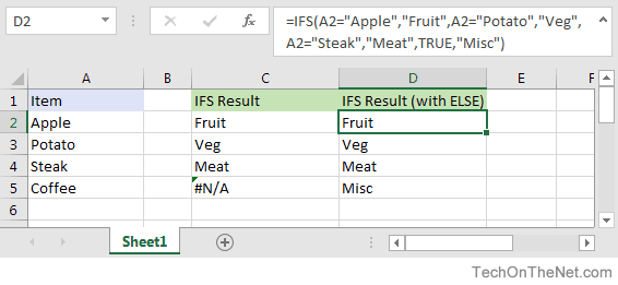
To avoid getting a #N/A error, create one final condition at the end of the formula that is TRUE and then place the value that you would like returned as the ELSE condition.
In this example, we have changed our formula from:
=IFS(A2="Apple","Fruit",A2="Potato","Veg",A2="Steak","Meat")
to
=IFS(A2="Apple","Fruit",A2="Potato","Veg",A2="Steak","Meat",TRUE,"Misc")
The addition of the final condition ,TRUE,"Misc" will allow us to return the value «Misc» when none of the previous conditions in the IFS function evaluate to TRUE.
The IFS function is a fantastic function and a great addition to Office 365 and Excel 2019. Give it a try!
The IFS function in Excel is a logical function that, in simplest terms, applies multiple IF functions. It allows the users to test a value against multiple conditions. The function accepts one or more conditions (or Boolean expressions) and a value to be returned against each condition.
The result returned by the function is the value that corresponds to the first condition, which evaluates to TRUE. IFS function is considered to be an easy and relatively simple alternative to the nested IF statements.
Syntax
The syntax of the IFS function is as follows:
=IFS(logical_test1, value_if_true1, [logical_test2], [value_if_true2], …)
Arguments:
logical_test1 – This is the first condition (or a Boolean expression) that the function needs to evaluate. If this condition is found to be TRUE, the function stops here and does not proceed to the next condition (if any). On the other hand, if the condition evaluates to FALSE, it moves on to compute the next condition (if any).value_if_true1 – This is the value that is returned if the ‘logical_test1’ turns out to be TRUE.[logical_test2] – This is an optional parameter that specifies the second test condition, which the function evaluates when the first condition turns out to be FALSE.[value_if_true2] – This is also an optional parameter that specifies the value that is returned if the first condition turns out to be FALSE and the second condition turns out to be TRUE.
Important Characteristics of IFS function
- The IFS function can support up to 127 conditions.
- If the conditions used inside the IFS function result in a value other than TRUE or FALSE, #VALUE! error is returned.
- If all the conditions within the IFS function evaluate to FALSE, then the function returns a #N/A error.
- If all the conditions within the function evaluate to FALSE, then a default value can be provided within the formula (we will see this with an example). However, the function does not support this out of the box, and this default value needs to be added with a condition that will always evaluate to TRUE (like 1=1 or TRUE, etc.)
Examples of the IFS function
Let us look at a few examples to understand the IFS function better.
Example 1 – Plain Vanilla Version of IFS Function
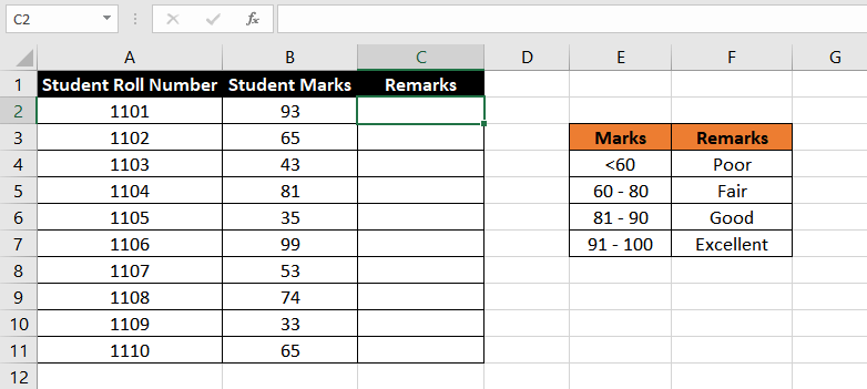
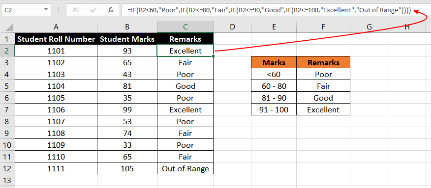
Consider a dataset consisting of three columns – Column 1 consists of ‘Student Roll Number’, Column 2 consists of ‘Student Marks’, and Column 3 consists of ‘Remarks’. Now, based on the ‘Student Marks’ column, we have to assign a specific remark against each student in the data set.
Let’s try to populate the ‘Remarks’ column based on the given conditions using the IFS function. In this case, the formula would be:
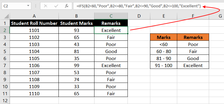
=IFS(B2<60,"Poor",B2<=80,"Fair",B2<=90,"Good",B2<=100,"Excellent")
Let’s try to wrap our heads around the formula and understand what is happening inside –
B2 is the cell containing data that has to be tested for the specified conditions, and the Remarks column needs to be populated based on its value.
The IFS function checks the first condition – if 93<60, which turns out to be FALSE. When this condition is found to be FALSE, it checks the next condition – if 93<=80, which again evaluates to be FALSE. When this condition is also found to be FALSE, it moves on to the next one to check – if 93<=90, this also turns out to be FALSE. Similarly, it checks for all conditions one by one until any one of the conditions evaluates to TRUE.
In this case, the condition 93<=100 yields the result TRUE, and so the value corresponding to it, i.e., «Excellent,» is populated in the ‘Remarks’ column.
This formula returns the required result against each student when we drag down the formula to all the other cells using the fill handle.
Example 2 – IFS Function with a Default Value
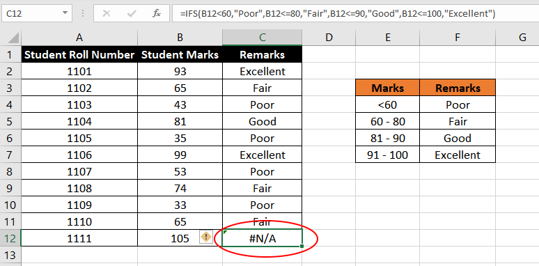
Now that this function returns the perfect value for each cell as required, what if the ‘logical_test’ argument does not match any of the given conditions?
For example, if there is another row that contains Student Marks as 105, there is no test condition in the given function that matches this value. In such a case, the function returns #N/A error.
Let’s look at this below.
IFS function does not provide a built-in way to have a default value to use when all conditions evaluate to FALSE. However, with some clever logic, we can add a default value within the IFS function to handle such cases.
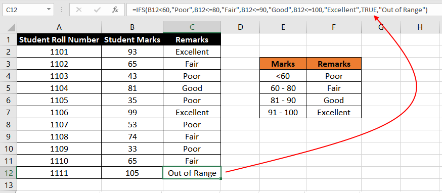
To add a default value, we have to add a condition to the function that always evaluates to TRUE – For example, 1=1, «A» = «A», or simply passing TRUE or 1 as the logic test would do the trick. Any value tied to such a condition would be displayed when no other condition matches.
Therefore, the formula can be modified as follows:
=IFS(B2<60,"Poor",B2<=80,"Fair",B2<=90,"Good",B2<=100,"Excellent",TRUE,"Out of Range")
Since the value 105 doesn’t fall under the specified conditions, the default value «Out of Range» is displayed.
Note: The default condition should always be the last condition in the IFS function.
IFS V/S Nested IF Statements
Before the introduction of the IFS function in MS Excel 2019, we used to have nested IF statements. The formulas using nested IF statements are much complicated when compared to the formulas using the IFS function. Let us try to use a nested IF formula for the same example stated above to understand this distinction.
With nested IF statements, the formula would be –
=IF(B2<60,"Poor",IF(B2<=80,"Fair",IF(B2<=90,"Good",IF(B2<=100,"Excellent","Out of Range"))))
This formula appears to be complicated using multiple parentheses and IF functions nested within one another, which is not the case with the IFS function. So, clearly, the IFS function is the winner here. It is relatively easier to write and understand when compared to multiple nested IF functions.
Recommended Reading – Excel If Function – How to Use
SWITCH function in Excel
The SWITCH function in Excel is similar to the IFS function. It compares one value (or the result of an expression) against a list of values and returns the result corresponding to the first exact match found. A default value can be specified at the end when no values match the given expression.
Syntax
The syntax of the SWITCH function is as follows:
=SWITCH(expression, value1, result1, [value2], [result2]…[default])
Arguments:
expression – The expression that is to be compared with other values/expressions.value1/result1 – SWITCH function compares the data using value/result pairs. The first value/result pair against which the expression has to be compared is given here.[value2]/[result2] – This is an optional parameter. It is the second value/result pair against which the expression has to be compared when the first comparison turns out to be FALSE.[default] – This is also an optional parameter. It refers to the default expression that appears when all the other comparisons turn out to be FALSE.
Example of SWITCH function
Let’s look at an example to understand the SWITCH function better.
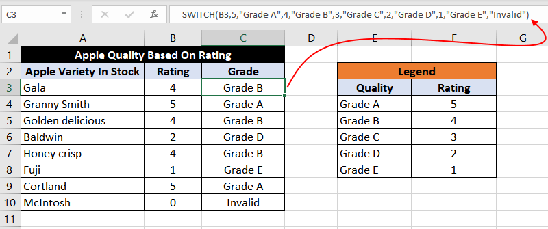
We have a dataset in the example with three columns «Apple Variety in Stock», «Rating» and «Grade» representing the quality of apples. Based on the rating we have to populate the quality of apples.
- Apples that are rated 5 are «Grade A» apples.
- Apples that are rated 4 are «Grade B» apples.
- Apples that are rated 3 are «Grade C» apples.
- Apples that are rated 2 are «Grade D» apples.
- Apples that are rated 1 are «Grade E» apples.
So, we use the following formula –
=SWITCH(B3,5,"Grade A",4,"Grade B",3,"Grade C",2,"Grade D",1,"Grade E","Invalid")
In this formula, the data in B3 is the expression that is to be compared against a set of value/result pairs.
The rating 5 is the first value against which data in B3 is compared. If the data in B3 matches 5, «Grade A» is returned as a result. If it turns out to be FALSE, it is compared against the next value, 4. If the data in B3 matches 4, «Grade B» is returned as a result.
If all evaluations turn out to be FALSE, the default value specified is returned. In this case, the default value specified is «Invalid».
Note: Up to 126 values/result pairs can be evaluated using the SWITCH function
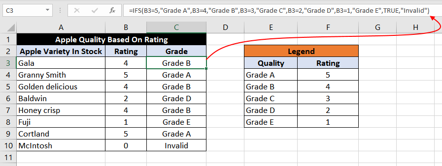
Now, let’s see how the IFS function can be used for the same example.
In this case, the formula would be –
=IFS(B3=5,"Grade A",B3=4,"Grade B",B3=3,"Grade C",B3=2,"Grade D",B3=1,"Grade E",TRUE,"Invalid")
The IFS function evaluates each condition and returns the corresponding result. And if no condition is found to be TRUE, the default value «Invalid» is populated in the required column.
IFS V/S SWITCH FUNCTION
Both IFS and SWITCH functions are very useful for testing. They evaluate multiple conditions and serve as an easy and quick alternative to the nested IF statements.
One minor edge of SWITCH over IFS is that the expression or the condition to be tested appears just once in the function and does not need to be repeated.
Another key difference between IFS and SWITCH functions is that the SWITCH function computes the exact match of the expression specified in the formula.
With SWITCH, you cannot use the logical operators like greater than (>) or less than (<) in the logic used to decide a match. For that reason, when an exact match is to be returned as a result, SWITCH could be a better option.
However, the IFS function can compute different logical expressions and return a value based on the logical computation. Thus, when the expressions have to be logically evaluated before returning a result, IFS serves as a great option.
That was all about the IFS function in Excel. I hope this tutorial will give you a confidence boost next time while dealing with the IFS function. I will see you soon with another amazing Excel function. Until then, keep Excelling.
Содержание
- IFS function
- Simple syntax
- Example 1
- Example 2
- Remarks
- Need more help?
- IFS Function
- Related functions
- Summary
- Purpose
- Return value
- Arguments
- Syntax
- Usage notes
- Structure
- Example #1 — grades, lowest to highest
- Example #2 — rating, highest to lowest
- Example #3 — default value
- IFS versus SWITCH
- IFS Function Examples – Excel & Google Sheets
- IFS Function Overview
- IFS function Syntax and inputs:
- What is the IFS Function?
- How to Use the IFS Function
- Setting a Default Value
- What IFS can return
- IFS in Google Sheets
- Как использовать функцию IFS в Excel?
- Что такое функция IFS Excel?
- Как использовать функцию IFS в Excel?
- Пример функции IFS с одним условием в Excel
- IFS Function
- What is the IFS Function?
- Formula
- How to use the IFS Function in Excel?
- Examples of the IFS Function in Excel
- Example 1 – Using IFS with ELSE
- Example 2 – IFS vs nested IF function
- A few pointers on the IFS function
- Additional Resources
IFS function
The IFS function checks whether one or more conditions are met, and returns a value that corresponds to the first TRUE condition. IFS can take the place of multiple nested IF statements, and is much easier to read with multiple conditions.
Note: This feature is available on Windows or Mac if you have Office 2019, or if you have a Microsoft 365 subscription. If you are a Microsoft 365 subscriber, make sure you have the latest version.
Simple syntax
Generally, the syntax for the IFS function is:
=IFS([Something is True1, Value if True1,Something is True2,Value if True2,Something is True3,Value if True3)
Please note that the IFS function allows you to test up to 127 different conditions. However, we don’t recommend nesting too many conditions with IF or IFS statements. This is because multiple conditions need to be entered in the correct order, and can be very difficult to build, test and update.
IFS(logical_test1, value_if_true1, [logical_test2, value_if_true2], [logical_test3, value_if_true3],…)
Condition that evaluates to TRUE or FALSE.
Result to be returned if logical_test1 evaluates to TRUE. Can be empty.
Condition that evaluates to TRUE or FALSE.
Result to be returned if logical_testN evaluates to TRUE. Each value_if_trueN corresponds with a condition logical_testN. Can be empty.
Example 1
The formula for cells A2:A6 is:
Which says IF(A2 is Greater Than 89, then return a «A», IF A2 is Greater Than 79, then return a «B», and so on and for all other values less than 59, return an «F»).
Example 2
The formula in cell G7 is:
Which says IF(the value in cell F2 equals 1, then return the value in cell D2, IF the value in cell F2 equals 2, then return the value in cell D3, and so on, finally ending with the value in cell D8 if none of the other conditions are met).
To specify a default result, enter TRUE for your final logical_test argument. If none of the other conditions are met, the corresponding value will be returned. In Example 1, rows 6 and 7 (with the 58 grade) demonstrate this.
If a logical_test argument is supplied without a corresponding value_if_true, this function shows a «You’ve entered too few arguments for this function» error message.
If a logical_test argument is evaluated and resolves to a value other than TRUE or FALSE, this function returns a #VALUE! error.
If no TRUE conditions are found, this function returns #N/A error.
Need more help?
You can always ask an expert in the Excel Tech Community or get support in the Answers community.
Источник
IFS Function
Summary
The Excel IFS function can run multiple tests and return a value corresponding to the first TRUE result. Use the IFS function to evaluate multiple conditions without multiple nested IF statements. IFS allows shorter, easier to read formulas.
Purpose
Return value
Arguments
- test1 — First logical test.
- value1 — Result when test1 is TRUE.
- test2, value2 — [optional] Second test/value pair.
Syntax
Usage notes
The IFs function evaluates multiple expressions and returns a result that corresponds to the first TRUE result. You can use the IFS function when you want a self-contained formula to test multiple conditions at the same time without nesting multiple IF statements. Formulas based on IFS are shorter and easier to read and write.
Conditions are provided to the IFS function as test/value pairs, and IFS can handle up to 127 conditions. Each test represents a logical test that returns TRUE or FALSE, and the value that follows will be returned when the test returns TRUE. In the event that more than one condition returns TRUE, the value corresponding to the first TRUE result is returned. For this reason, it is important to consider the order in which conditions appear.
Structure
An IFS formula with 3 tests can be visualized like this:
A value is returned by IFS only when the previous test returns TRUE, and the first test to return TRUE «wins». For better readability, you can add line breaks to an IFS formula as shown above.
Note: the IFS function does not provide an argument for a default value. See Example #3 below for a workaround.
Example #1 — grades, lowest to highest
In the example shown below, the IFS function is used to assign a grade based on a score. The formula in E5, copied down, is:
Notice the conditions are entered «in order» to test lower scores first. The grade associated with the first test to return TRUE is returned.
Example #2 — rating, highest to lowest
In a simple rating system, a score of 3 or greater is «Good», a score between 2 and 3 is «Average», and anything below 2 is «Poor». To assign these values with IFS, three conditions are used:
Notice in this case conditions are arranged to test higher values first.
Example #3 — default value
The IFS function does not have a built-in default value to use when all conditions are FALSE. However, to provide a default value, you can enter TRUE as a final test, followed by a value to use as a default.
In the example below, a status code of 100 is «OK», a code of 200 is «Warning», and a code of 300 is «Error». Any other code value is invalid, so TRUE is provided as the final test, and «Invalid» is provided as a «default» value.
When the value in A1 is 100, 200, or 300, IFS will return the messages shown above. When A1 contains any other value (including when A1 is empty) IFS will return «Invalid». Without this final condition, IFS will return #N/A when a code is not recognized.
Note: IFS is a new function available in Excel 365 and Excel 2019.
IFS versus SWITCH
Like the SWITCH function, the IFS function allows you to test more than one condition in a single self-contained formula. Both functions make it easier to write (and read) a formula with many conditions. One advantage of SWITCH over IFS is that the expression appears just once in the function and does not need to be repeated. In addition, SWITCH can accept a default value. However, SWITCH is limited to exact matching. It is not possible to use operators like greater than (>) or less than (
Источник
IFS Function Examples – Excel & Google Sheets
This tutorial demonstrates how to use the IFS Function in Excel and Google Sheets.
IFS Function Overview
The Excel IFS function runs multiple tests and returns a value corresponding to the first TRUE result.
To use the IFS Excel Worksheet Function, select a cell and type:
(Notice how the formula inputs appear)
IFS function Syntax and inputs:
test1 – First logical test.
value1 – Result when test1 is TRUE.
test2, value2 – [optional] Second test/value pair.
What is the IFS Function?
IFS is a “conditional” function. You define a series of logical tests, each with a return value associated with it. Excel works through each of your tests in turn, and as soon as it finds one that evaluates to TRUE, it returns the value you associated with that test.
This works much the same was as when nesting multiple IF statements, but tends to be easier to read and work with.
How to Use the IFS Function
You use the Excel IFS Function like this:
This formula takes a student’s test score, and converts it into their grade for that test.
The formula may look complicated, but it makes more sense if you put each test on a separate line:
That’s better! It’s much clearer now that we have a series of tests paired with a return value. Excel works down the list until it gets a match, and then returns the grade that we’ve paired with that score.
You can define up to 127 tests in the IFS Function.
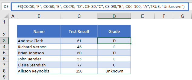
Setting a Default Value
With the normal IF statement, we define two values that Excel can return: one for when the logical test is true, and another for when it is false.
IFS doesn’t have the option to add a false return value, and if Excel doesn’t find a match in any of your tests, it will return #N/A. Not good. But, we can get around this by setting a default value.
It works like this:
We’ve set up a final logical test – just “TRUE”, by itself.
TRUE, naturally, evaluates to TRUE. So, if Excel doesn’t find a match in our previous tests, the final test will always be triggered, and Excel will return “Unknown.”
What IFS can return
Above we told IFS to return a text string – the grade associated with each test score. But you can also return numbers, or even other formulas.
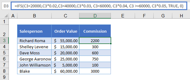
For example, if you have a sales team, and you pay them commission based on the value of each sale, you could use IFS to calculate their commission according to the sale value.
Now IFS will check the value in C3, and then return the associated formula when it finds a match. So sales below $20,000 earn 2% interest, below $40,000 earns 3%, and so on.
For good measure, we’ve also set a default value of 0.
IFS in Google Sheets
The IFS Function works exactly the same in Google Sheets as in Excel:
Источник
Как использовать функцию IFS в Excel?
Добрый день, друзья. Функция IFS Excel позволяет легко создавать до 127 вложенных операторов IF в одной формуле. Вот как ее использовать. Условные функции, такие как IFS, потенциально могут вывести ваши формулы Excel на новый уровень. С помощью IFS можно создавать условия и вкладывать различные опции друг в друга в одной формуле. Кроме того, есть возможность применять опцию IFS самостоятельно.
Но что такое опция IFS и чем она отличается от простой опции IF? Читайте дальше, чтобы узнать, что значит IFS в Excel и как её правильно применять?
Что такое функция IFS Excel?
Опция IFS в Excel принимает значения и проверяет их на соответствие заданным параметрам. Если этот параметр удовлетворяет первому условию, то формула останавливается на этом и выдает вывод. Но, если первое условие не выполнено, формула будет продолжать последовательно проверять условия до тех пор, пока не будет выполнено условие.
=IFS([Something is True1, Output if True1,Something is True2,Output if True2,Something is True3,Output if True3)
Если значение не соответствует ни одному из условий, то формула возвращает ошибку N/A. Однако вы можете исправить это, введя конечное условие, такое как TRUE, и вывод для этого условия, например «Значение не соответствует ни одному из условий». Условие TRUE гарантирует, что любое значение соответствует, по крайней мере, конечному условию, чтобы вы не получили ошибку N / A.
Как использовать функцию IFS в Excel?
IFS — это обновленная версия функции IF в Excel. Синтаксис и использование аналогичны, за исключением того, что IFS предназначена для работы в нескольких условиях. Функция IF требовала вложения нескольких функций IF для определения нескольких условий, в то время как IFS может определить все это с помощью одной функции.
Первым параметром в IFS будет условие, а вторым параметром будет результат, если это условие выполнено. Третьим параметром будет условие номер 2, а четвертым параметром будет результат, если условие номер 2 выполнено.
Параметры объединяются таким образом, и создаётся возможность для ввода до 127 условий в одной опции IFS. Разумеется, можно также ввести другую опцию в выходные данные для создания составных вложенных формул. Если вы работали с формулами IF и nested IF, то использование IFS будет для вас легким делом. IFS здесь, чтобы упростить задачу, так что позвольте ей это сделать!
Пример функции IFS с одним условием в Excel
Чтение о функции IFS не принесет вам никакой пользы, пока вы не примените ее на практике. Итак, давайте начнем с примера. Несмотря на то, что функция IFS может работать в нескольких условиях, это не означает, что вы не можете использовать ее для сценариев с одним условием. Давайте напишем формулу IFS с одним условием и даже включим в нее некоторые другие функции, чтобы разобраться.
В этом примере у нас есть некоторые продукты и годы их производства. Эти воображаемые продукты портятся через два года после их производства, поэтому мы собираемся создать формулу, которая определяет, просрочены продукты или нет. Конечно же, мы будем применять опцию IFS вместе с опциями YEAR и TODAY .
Функция YEAR выводит год с определенной даты. Мы собираемся предоставить функции YEAR сегодняшнюю дату, используя функцию TODAY, чтобы вывод комплекса YEAR(TODAY()) относился к текущему году. Давайте начнем.
Источник
IFS Function
Returns a value that meets the first TRUE condition
What is the IFS Function?
The IFS Function[1] in Excel is a Logical function that was introduced in Excel 2016. The function is an alternative to the Nested IF function and is much easier to use. The IFS function checks if one or more than one conditions are observed or not and accordingly returns a value that meets the first TRUE condition.
Formula
= IFS(logical_test1, Value1 [logical_test2, Value2] …, [logical_test127, Value127])
- Logical_test1 – First logical test. This is a required argument and is the condition that is used by Excel to evaluate whether it is TRUE or FALSE.
- Value1 – Result when logical_test1 is true. If required, you can keep it empty.
The rest of the logical_test and Value arguments are optional. The function allows the user to put in up to 127 logical_test arguments using the IFS function.
How to use the IFS Function in Excel?
It is a built-in function that can be used as a worksheet function in Excel. Let’s take a look at an example:
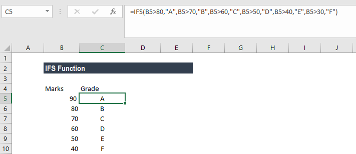
Assume we wish to assign grades to marks earned by students. We can use the IFS Function in the following manner:
The formula used is:
IFS(A2>80,”A”,A2>70,”B”,A2>60,”C”,A2>50,”D”,A2>40,”E”,A2>30,”F”), which says that if cell A2 is greater than 80 then return an “A” and so on.
Using this formula, the result would be:
Examples of the IFS Function in Excel
To understand the uses of this function, let’s consider a few more examples:
Example 1 – Using IFS with ELSE
Assume we have a list of items and we need to classify them under four common headings: Vegetable, Fruit, Green Vegetable, and Beverage. When we use the IFS function and give the formula =IFS(A2=”Apple”,”Fruit”,A2=”Banana”,”Fruit”,A2=”Spinach”,”Green Vegetable”,A2=”coffee”,”Beverage”,A2=”cabbage”,”Green Vegetable”,A2=”capsicum”,”Vegetable”)
Then, we will get the following result:
In this example, we have entered multiple logical tests in the IFS function. When a logical test evaluates to TRUE, the corresponding value will be returned. However, if none of the logical tests evaluate to TRUE, then IFS function would give #N/A error. This is what we got for Pepper in B8.
Using the ELSE function, we can ensure that this #N/A error is removed. For this, we would place a final logical test at the end of the formula that is TRUE and then place a value that shall be returned.
Here, we added TRUE, “Misc”, this will ensure that Excel returns the value “Misc” in the scenario where none of the previous logical tests in the IFS function evaluates to TRUE.
Now the results would as be as shown below:
Example 2 – IFS vs nested IF function
Prior to the introduction of the IFS function in Excel, we used to use nested IF function. Let’s see how the IFS function is superior to nested IF. Let’s assume we wish to give discounts to customers based on their total purchases from us. So, a customer would get a 5% discount for purchases more than $100 but less than $500, a 10% discount if he made purchases of more than $500 but less than $750, 20% if he made purchases of more than $750 but less than $1,000, and 30% for all purchases above $1,000.
Let’s see the formula when we would have used nested IF function:
Now, let’s see how it becomes easy to write the formula for same results using IFS:
Hence, IFS is easier, as it allows using a single function to input a series of logical tests. It becomes cumbersome in the nested IF function, especially when we use a large number of logical tests.
A few pointers on the IFS function
- #N/A Error occurs when no TRUE conditions are found by IFS function.
- #VALUE! Error – We will get this error when the logical_test argument resolves to a value other than TRUE or FALSE.
- “You’ve entered too few arguments for this function” error message – This message appears when we provide a logical_test argument without a corresponding value.
Additional Resources
Thank you for reading CFI’s guide on the IFS Function. To learn more, check out these additional CFI resources:
Источник

