
Excel for Microsoft 365 Excel for Microsoft 365 for Mac Excel 2021 Excel 2021 for Mac Excel 2019 Excel 2019 for Mac Excel 2016 Excel 2016 for Mac Excel 2013 Excel 2010 Excel 2007 Excel for Mac 2011 More…Less
By using What-If Analysis tools in Excel, you can use several different sets of values in one or more formulas to explore all the various results.
For example, you can do What-If Analysis to build two budgets that each assumes a certain level of revenue. Or, you can specify a result that you want a formula to produce, and then determine what sets of values will produce that result. Excel provides several different tools to help you perform the type of analysis that fits your needs.
Note that this is just an overview of those tools. There are links to help topics for each one specifically.
What-If Analysis is the process of changing the values in cells to see how those changes will affect the outcome of formulas on the worksheet.
Three kinds of What-If Analysis tools come with Excel: Scenarios, Goal Seek, and Data Tables. Scenarios and Data tables take sets of input values and determine possible results. A Data Table works with only one or two variables, but it can accept many different values for those variables. A Scenario can have multiple variables, but it can only accommodate up to 32 values. Goal Seek works differently from Scenarios and Data Tables in that it takes a result and determines possible input values that produce that result.
In addition to these three tools, you can install add-ins that help you perform What-If Analysis, such as the Solver add-in. The Solver add-in is similar to Goal Seek, but it can accommodate more variables. You can also create forecasts by using the fill handle and various commands that are built into Excel.
For more advanced models, you can use the Analysis ToolPak add-in.
A Scenario is a set of values that Excel saves and can substitute automatically in cells on a worksheet. You can create and save different groups of values on a worksheet and then switch to any of these new scenarios to view different results.
For example, suppose you have two budget scenarios: a worst case and a best case. You can use the Scenario Manager to create both scenarios on the same worksheet, and then switch between them. For each scenario, you specify the cells that change and the values to use for that scenario. When you switch between scenarios, the result cell changes to reflect the different changing cell values.
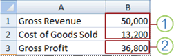
1. Changing cells
2. Result cell
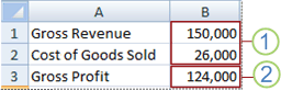
1. Changing cells
2. Result cell
If several people have specific information in separate workbooks that you want to use in scenarios, you can collect those workbooks and merge their scenarios.
After you have created or gathered all the scenarios that you need, you can create a Scenario Summary Report that incorporates information from those scenarios. A scenario report displays all the scenario information in one table on a new worksheet.
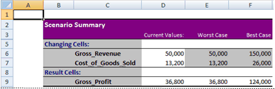
Note: Scenario reports are not automatically recalculated. If you change the values of a scenario, those changes will not show up in an existing summary report. Instead, you must create a new summary report.
If you know the result that you want from a formula, but you’re not sure what input value the formula requires to get that result, you can use the Goal Seek feature. For example, suppose that you need to borrow some money. You know how much money you want, how long a period you want in which to pay off the loan, and how much you can afford to pay each month. You can use Goal Seek to determine what interest rate you must secure in order to meet your loan goal.

Cells B1, B2, and B3 are the values for the loan amount, term length, and interest rate.
Cell B4 displays the result of the formula =PMT(B3/12,B2,B1).
Note: Goal Seek works with only one variable input value. If you want to determine more than one input value, for example, the loan amount and the monthly payment amount for a loan, you should instead use the Solver add-in. For more information about the Solver add-in, see the section Prepare forecasts and advanced business models, and follow the links in the See Also section.
If you have a formula that uses one or two variables, or multiple formulas that all use one common variable, you can use a Data Table to see all the outcomes in one place. Using Data Tables makes it easy to examine a range of possibilities at a glance. Because you focus on only one or two variables, results are easy to read and share in tabular form. If automatic recalculation is enabled for the workbook, the data in Data Tables immediately recalculates; as a result, you always have fresh data.
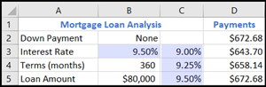
Cell B3 contains the input value.
Cells C3, C4, and C5 are values Excel substitutes based on the value entered in B3.
A Data Table cannot accommodate more than two variables. If you want to analyze more than two variables, you can use Scenarios. Although it is limited to only one or two variables, a Data Table can use as many different variable values as you want. A Scenario can have a maximum of 32 different values, but you can create as many scenarios as you want.
If you want to prepare forecasts, you can use Excel to automatically generate future values that are based on existing data, or to automatically generate extrapolated values that are based on linear trend or growth trend calculations.
You can fill in a series of values that fit a simple linear trend or an exponential growth trend by using the fill handle or the Series command. To extend complex and nonlinear data, you can use worksheet functions or the regression analysis tool in the Analysis ToolPak Add-in.
Although Goal Seek can accommodate only one variable, you can project backward for more variables by using the Solver add-in. By using Solver, you can find an optimal value for a formula in one cell—called the target cell—on a worksheet.
Solver works with a group of cells that are related to the formula in the target cell. Solver adjusts the values in the changing cells that you specify—called the adjustable cells—to produce the result that you specify from the target cell formula. You can apply constraints to restrict the values that Solver can use in the model, and the constraints can refer to other cells that affect the target cell formula.
Need more help?
You can always ask an expert in the Excel Tech Community or get support in the Answers community.
See Also
Scenarios
Goal Seek
Data Tables
Using Solver for capital budgeting
Using Solver to determine the optimal product mix
Define and solve a problem by using Solver
Analysis ToolPak Add-in
Overview of formulas in Excel
How to avoid broken formulas
Detect errors in formulas
Keyboard shortcuts in Excel
Excel functions (alphabetical)
Excel functions (by category)
Need more help?
What-If Analysis in Excel is a tool that helps us create different models, scenarios, and Data Tables. This article will look at the ways of using What-If Analysis.
Table of contents
- What is a What-If Analysis in Excel?
- #1 Scenario Manager in What-If Analysis
- #2 Goal Seek in What-If Analysis
- #3 Data Table in What-If Analysis
- Things to Remember
- Recommended Articles
We have three parts of What-If Analysis in Excel. They are as follows:
- Scenario Manager
- Goal Seek in Excel
- Data Table in Excel
You can download this What-If Analysis Excel Template here – What-If Analysis Excel Template
#1 Scenario Manager in What-If Analysis
As a business head, it is important to know the different scenarios of your future project. Based on the scenarios, the business head will make decisions. For example, you are going to undertake one of the important projects. You have done your homework and listed all the possible expenditures from your end, and below is the list of all your expenses.
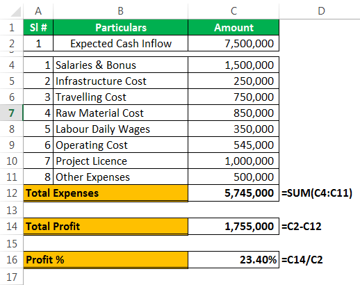
The expected cash flow from this project is $75 million, which is in cell C2. Total expenses comprise all your fixed and variable expenses, the total cost is $57.45 million in cell C12. Total profit is $17.55 million in cell C14, and profit % is 23.40% of your cash inflow.
It is the basic scenario of your project. Now, you need to know the profit scenario if some of your expenses increase or decrease.
Scenario 1
- In a general case scenario, you have estimated the “Project License” cost to be $10 million, but you are sure anticipating it to be $15 million
- Raw material costs to be increased by $2.5 million
- Other expensesOther expenses comprise all the non-operating costs incurred for the supporting business operations. Such payments like rent, insurance and taxes have no direct connection with the mainstream business activities.read more to be decreased by 50 thousand.
Scenario 2
- The “Project Cost” to be at $20 million
- The “Labor Daily Wages” to be at $5 million
- The “Operating Cost” is to be at $3.5 million
Now, you have listed out all the scenarios in the form. Based on these scenarios, you need to create a table about how it will impact your profit and profit %.
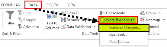
To create What-If Analysis scenarios, follow the below steps.
- Go to DATA > What-If Analysis > Scenario Manager.

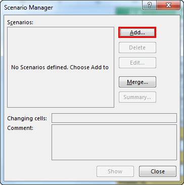
- Once you click “Scenario Manager,” it will show you below the dialog box.

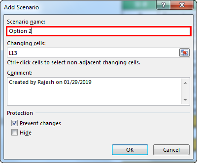
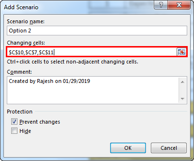
- Click on “Add.” Then, give “Scenario name.”

- In changing cells, select the first scenario changes you have listed out. The changes are Project License (cell C10) at $15 million, Raw Material Cost (cell C7) at $11 million, and Other Expenses (cell C11) at $4.5 million. Mention these three cells here.
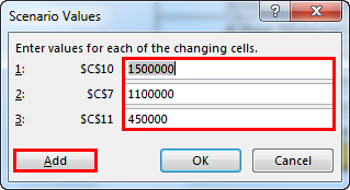
- Click on “OK.” It will ask you to mention the new values as listed in scenario 1.

- Do not click on “OK” but click on “OK Add.” It will save this scenario for you.
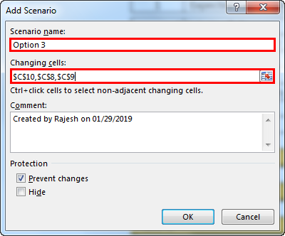
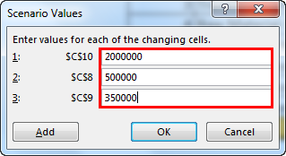
- Now, it will ask you to create one more scenario. As we listed in scenario 2, make the changes. This time we need to change Project Cost (C10), Labour Cost (C8), and Operating Cost (C9).
- Now, add new values here.
- Now click on “OK.” It will show all the scenarios we have created.
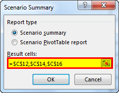
- Click on “Scenario summary.” It will ask you which result cells you want to change. Here, we need to change the Total Expense Cell (C12), Total Profit Cell (C14), and Profit % cell (C16).

- Click on “OK.” It will create a summary report for you in the new worksheet.


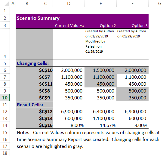
Total Excel has created three scenarios even though we have supplied only two scenario changes because Excel will show existing reports as one scenario.
From this table, we can easily see the impact of changes in pour profit %.
#2 Goal Seek in What-If Analysis
Now, we know the Scenario Manager’s advantage. What-if-Analysis Goal Seek can tell you what you must do to achieve the target.
Andrew is a class 10th student. His target is to achieve an average score of 85 in the final exam. He has already completed 5 exams and left with only 1 exam. Therefore, in the completed 5 exams.
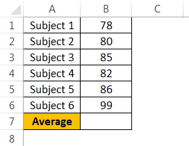
To calculate the current average, apply the average formula in the B7 cell.
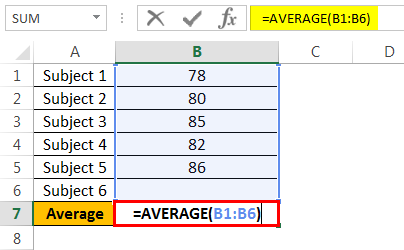
The current average is 82.2.
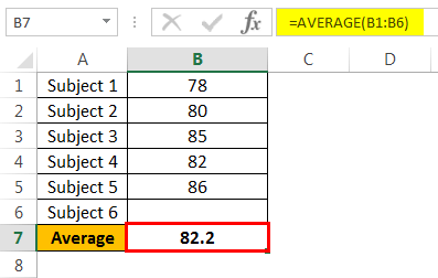
Andrew’s GOAL is 85. His current average is 82.2. He is short by 3.8 with one exam.
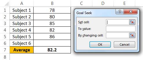
Now, the question is how much he has to score in the final exam to eventually get an overall average of 85. It can be found by the What-If Analysis GOAL SEEK tool.
- Step 1: Go to DATA > What-If Analysis > Goal Seek.

- Step 2: It will show you below the dialog box.
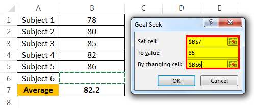
- Step 3: Here, we need to set the cell first. “Set cell” is nothing but which cell we need for the final result, i.e., our overall average cell (B7). Next is “To value.” Again, Andrew’s overall average GOAL is nothing but for what value we need to set the cell (85).
The next and final step is changing which cell you want to see the impact on. So, we need to change cell B6, the cell for the final subject’s score.
- Step 4: Click on “OK.” Excel will take a few seconds to complete the process, but it eventually shows the result like the one below.
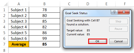
Now, we have our results here. To get an overall average of 85, Andrew has to score 99 in the final exam.
#3 Data Table in What-If Analysis
We have already seen two wonderful techniques under What-If Analysis in Excel. First, the Data Table can create different scenario tables based on the variable change. We have two kinds of Data Tables here: one variable Data Table and a “Two-variable data tableA two-variable data table helps analyze how two different variables impact the overall data table. In simple terms, it helps determine what effect does changing the two variables have on the result.read more.” This article will show you One variable data table in ExcelOne variable data table in excel means changing one variable with multiple options and getting the results for multiple scenarios. The data inputs in one variable data table are either in a single column or across a row.read more.
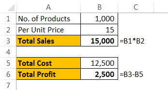
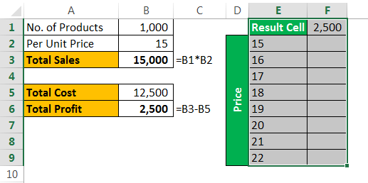
Assume you are selling 1,000 products at ₹15, your total anticipated expense is ₹12,500, and your profit is ₹2,500.
You are not happy with the profit you are getting. Your anticipated profit is ₹7,500. You have decided to increase your per-unit price to increase your profit, but you do not know how much you need to increase.
Data tables can help you. Create a table below.

Now, in the cell, F1 links to the “Total Profit” cell, B6.

- Step 1: Select the newly created table.
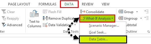
- Step 2: Go to DATA > What-if Analysis > Data Table.
- Step 3: Now, you will see below dialog box.
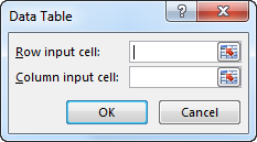
- Step 4: Since we are showing the result vertically, leave the ”Row input cell.” In the “Column input cell,” select cell B2, which is the original selling price.
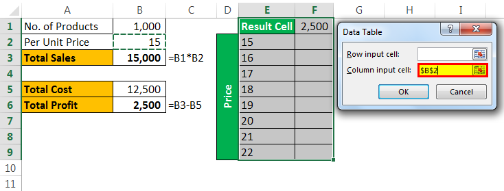
- Step 5: Click on “OK” to get the results. It will list out profit numbers in the new table.
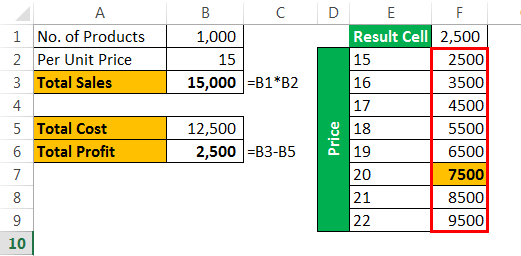
So, we have our Data Table ready. To profit from ₹7,500, you need to sell at ₹20 per unit.
Things to Remember
- The What-If Analysis data table can be performed with two variable changes. Refer to our article on What-If Analysis two-variable Data Table.
- What-If Analysis Goal Seek takes a few seconds to perform calculations.
- What-If Analysis Scenario Manager can give a summary with input numbers and current values together.
Recommended Articles
This article is a guide to What-If Analysis in Excel. Here, we discuss three types of What-If Analysis in Excel such as 1) Scenario Manager, 2) Goal Seek, 3) Data Tables along with practical examples, and a downloadable Excel template. You may learn more about Excel from the following articles: –
- Pareto Analysis in ExcelA pareto chart is a graph which is a combination of a bar graph and a line graph, indicates the defect frequency and its cumulative impact. It helps in finding the defects to observe the best possible and overall improvement measure.read more
- Goal Seek in VBA
- Sensitivity Analysis in Excel
Create Different Scenarios | Scenario Summary | Goal Seek
What-If Analysis in Excel allows you to try out different values (scenarios) for formulas. The following example helps you master what-if analysis quickly and easily.
Assume you own a book store and have 100 books in storage. You sell a certain % for the highest price of $50 and a certain % for the lower price of $20.

If you sell 60% for the highest price, cell D10 calculates a total profit of 60 * $50 + 40 * $20 = $3800.
Create Different Scenarios
But what if you sell 70% for the highest price? And what if you sell 80% for the highest price? Or 90%, or even 100%? Each different percentage is a different scenario. You can use the Scenario Manager to create these scenarios.
Note: You can simply type in a different percentage into cell C4 to see the corresponding result of a scenario in cell D10. However, what-if analysis enables you to easily compare the results of different scenarios. Read on.
1. On the Data tab, in the Forecast group, click What-If Analysis.

2. Click Scenario Manager.

The Scenario Manager dialog box appears.
3. Add a scenario by clicking on Add.

4. Type a name (60% highest), select cell C4 (% sold for the highest price) for the Changing cells and click on OK.

5. Enter the corresponding value 0.6 and click on OK again.

6. Next, add 4 other scenarios (70%, 80%, 90% and 100%).
Finally, your Scenario Manager should be consistent with the picture below:

Note: to see the result of a scenario, select the scenario and click on the Show button. Excel will change the value of cell C4 accordingly for you to see the corresponding result on the sheet.
Scenario Summary
To easily compare the results of these scenarios, execute the following steps.
1. Click the Summary button in the Scenario Manager.
2. Next, select cell D10 (total profit) for the result cell and click on OK.

Result:

Conclusion: if you sell 70% for the highest price, you obtain a total profit of $4100, if you sell 80% for the highest price, you obtain a total profit of $4400, etc. That’s how easy what-if analysis in Excel can be.
Goal Seek
What if you want to know how many books you need to sell for the highest price, to obtain a total profit of exactly $4700? You can use Excel’s Goal Seek feature to find the answer.
1. On the Data tab, in the Forecast group, click What-If Analysis.
2. Click Goal Seek.

The Goal Seek dialog box appears.
3. Select cell D10.
4. Click in the ‘To value’ box and type 4700.
5. Click in the ‘By changing cell’ box and select cell C4.
6. Click OK.

Result. You need to sell 90% of the books for the highest price to obtain a total profit of exactly $4700.

Note: visit our page about Goal Seek for more examples and tips.
Lesson 21: Using What-If Analysis
/en/excel2010/creating-pivottables/content/
Introduction
Let’s saying you’re trying to solve a complicated problem with Excel, like calculating an unknown value. You could try solving it on your own, plugging in different numbers until you find the right answer. However, this method could take a lot of time and effort.
Instead of calculating the answer by yourself, you could use a powerful Excel tool called what-if analysis. This feature makes it easier to experiment with your data. In this lesson, we’ll show you how to use what-if analysis to answer different types of questions.
What-if analysis
Excel includes many powerful tools to perform complex mathematical calculations, including what-if analysis. This feature can help you experiment and answer questions with your data, even when the data is incomplete. In this lesson, you’ll learn how to use a what-if analysis tool called Goal Seek.
Optional: You can download this example for extra practice.
Using Goal Seek
When you create a formula or function in Excel, you put various parts together to calculate a result. Goal Seek works in the opposite way: It lets you start with the desired result, and it calculates the input value that will give you that result. We’ll use a few examples to show how to use Goal Seek.
To use Goal Seek (Example 1):
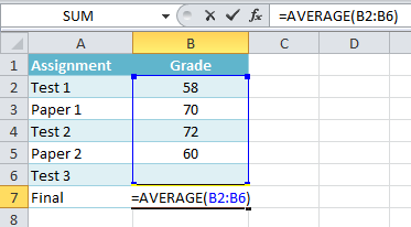
Let’s say you’re enrolled in a class. You currently have a grade of 65, and you need at least a 70 to pass the class. Luckily, you have one final assignment that might be able to raise your average. You can use Goal Seek to find out what grade you need on the final assignment to pass the class.
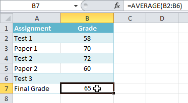
In the image below, you can see that the grades on the first four assignments are 58, 70, 72, and 60. Even though we don’t know what the fifth grade will be, we can go ahead and write a formula or function that calculates the final grade. In this case, each assignment is weighted equally, so all we have to do is average all five grades by typing =AVERAGE(B2:B6). Once we use Goal Seek, cell B6 will show us the minimum grade we’ll need to make on the final assignment.
 Function calculating the monthly payment
- Select the cell containing the value you want to change. When you use Goal Seek, you’ll need to select a cell that already contains a formula or function. In our example, we’ll select cell B7 because it contains the formula =AVERAGE(B2:B6).
 Selecting cell B7
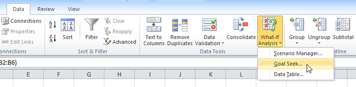
 - From the Data tab, click the What-If Analysis command, then select Goal Seek from the drop-down menu.
 Selecting Goal Seek from the drop-down menu
 - A dialog box will appear with three fields:
- Set cell: This is the cell that will contain the desired result. In our example, cell B7 is already selected.
- To value: This is the desired result. In our example, we’ll enter 70 because we need to earn at least that to pass the class.
- By changing cell: This is the cell where Goal Seek will place its answer. In our example, we’ll select cell B6 because we want to determine the grade we need to earn on the final assignment.
- When you’re done, click OK.
 Entering the desired values into the dialog box and clicking OK
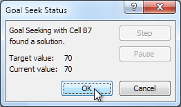
 - The dialog box will tell you if Goal Seek was able to find a solution. Click OK.
Clicking OK
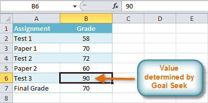
- The result will appear in the specified cell. In our example, Goal Seek calculated that we will need to score at least a 90 on the final assignment to earn a passing grade.
 The completed Goal Seek and calculated value

To use Goal Seek (Example 2):
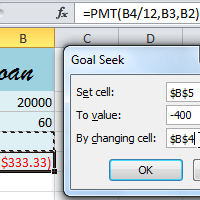
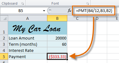
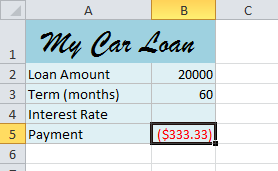
Let’s say you need a loan to buy a new car. You already know you want a loan amount of $20,000, a 60-month term—the length of time it takes to pay off the loan—and a payment of no more than $400 per month. However, you’re not sure yet what the interest rate will be.
In the image below, you can see that Interest Rate is left blank and Payment is $333.33. This is because the payment is being calculated by a specialized function called the PMT (Payment) function, and $333.33 is what the monthly payment would be if there were no interest ($20,000 divided by 60 monthly payments).
 Function calculating the monthly payment
If we typed different values into the empty Interest Rate cell, we could eventually find the value that causes Payment to be $400, and that would be the highest interest rate that we could afford. However, Goal Seek can do this automatically by starting with the result and working backward.
To insert the PMT function:
- Select the cell where you want the function to be.
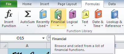
- From the Formula tab, select the Financial command.
 The Financial command
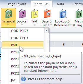
 - A drop-down menu will appear showing all financial-related functions. Scroll down and select the PMT function.
 Selecting the PMT function
 - A dialog box will appear.
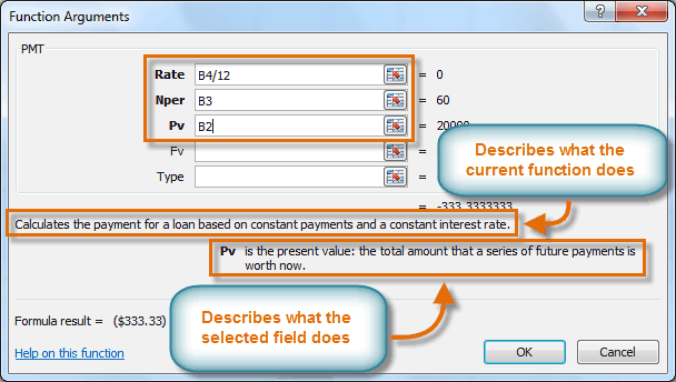
- Enter the desired values and/or cell references into the different fields. In this example, we’re only using Rate, Nper (the number of payments), and Pv (the loan amount).
 Entering values into the necessary fields
 - Click OK. The result will appear in the selected cell. Note that this is not our final result because we still don’t know what the interest rate will be.
 The monthly payment, not including interest
To use Goal Seek to find the interest rate:
Now that we’ve added the PMT function, we can use Goal Seek to find the interest rate we’ll need.
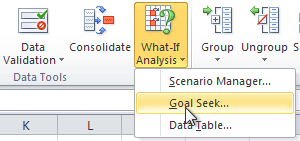
- From the Data tab, click the What-If Analysis command.
- Select Goal Seek.
 Selecting Goal Seek
 - A dialog box will appear containing three fields:
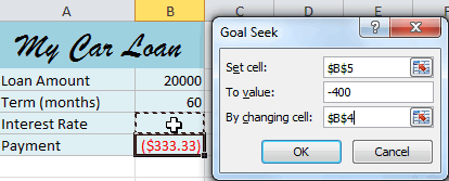
- Set cell: This is the cell that will contain the desired result (in this case, the monthly payment). In this example, we will set it to B5 (it doesn’t matter whether it’s an absolute or relative reference).
- To value: This is the desired result. We’ll set it to -400. Because we’re making a payment that will be subtracted from our loan amount, we have to enter the payment as a negative number.
- By changing cell: This is the cell where Goal Seek will place its answer (in this case, the interest rate). We’ll set it to B4.
 Entering values into the Goal Seek fields
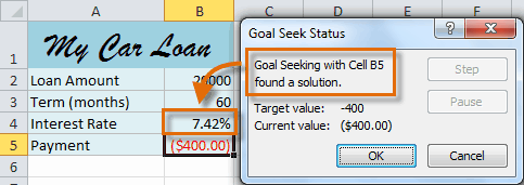
 - When you’re done, click OK. The dialog box will tell you whether Goal Seek was able to find a solution. In this example, the solution is 7.42%, and it has been placed in cell B4. This tells us that a 7.42% interest rate will give us a $400-per-month payment on a $20,000 loan that is paid off over five years, or 60 months.
 Solution found by Goal Seek
Other types of what-if analysis
For more advanced projects, you may want to consider the other types of what-if analysis: scenarios and data tables. Rather than start from the desired result and working backward like with Goal Seek, you can use these options to test multiple values and see how the results change.
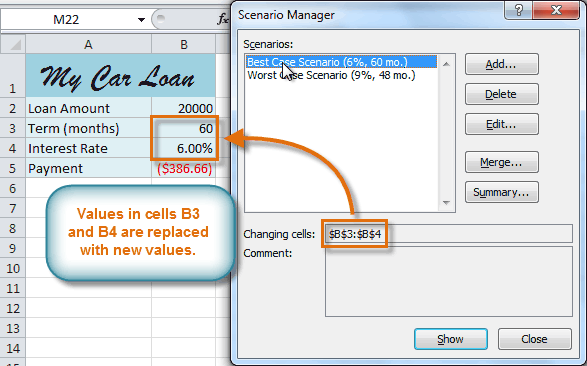
- Scenarios let you substitute values for multiple cells (up to 32) at the same time. You can create as many scenarios as you want and then compare them without changing the values manually. In the example below, each scenario contains a term and an interest rate. When each scenario is selected, it will replace the values in the spreadsheet with its own values, and the result will be recalculated.
 Using the Scenario Manager to compare different options
For more information on scenarios, check out this article from Microsoft.
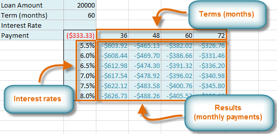
- Data tables allow you to take one or two variables in a formula and replace them with as many different values as you want, then view the results in a table. This option is especially powerful because it shows multiple results at the same time, unlike scenarios or Goal Seek. In the example below, we can view 24 possible results for a car loan.
 Data tables
For more information on data tables, check out this article from Microsoft.
Challenge!
- Open an existing Excel 2010 workbook. If you want, you can use this example.
- Use Goal Seek to determine an unknown value. If you’re using the example, go to the History Class worksheet and use Goal Seek to determine what grade you would need on Test 3 to earn a final grade average of 90.
- Insert the PMT function into the worksheet. If you are using the example, go to the Car Loan worksheet and insert the function into cell B5.
- Use Goal Seek to find the interest rate you’ll need in order to have a monthly payment of $400. What interest rate would you need if you could only afford a $380 monthly payment?
/en/excel2010/merging-copies-of-a-shared-workbook/content/
If you’ve ever experimented with different variables to see how your changes would affect the outcome of a situation, you’ve done a what if analysis.
Would you be able to sell more items if you had a sale this week? Or would you make more money by increasing the price instead? In the above scenarios, you want to know the degree to which each change affects the overall outcome. For this reason, a what if analysis is also known as a sensitivity analysis.
Most what if analyses are really mathematical calculations, and that is Excel’s specialty. To help you do a what if analysis, Excel uses commands from the Forecast command group on the Data tab to prepare simple forecasts or advanced business models.
Download your free Excel practice file
Use this free Excel file to practice what if analysis along with the tutorial.
Goal Seek
The simplest sensitivity analysis tool in Excel is Goal Seek. Assuming that you know the single outcome you would like to achieve, the Goal Seek feature in Excel allows you to arrive at that goal by mathematically adjusting a single variable within the equation.
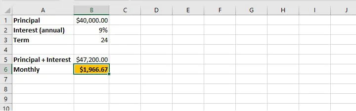
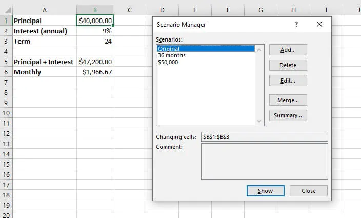
 To illustrate how it works, imagine that the bank is offering an interest rate of 9% per annum on personal loans with 24 months to repay, and that you would like to borrow $40,000.
Using the above information, the bank calculates that the amount borrowed plus interest over the loan period will be $47,200, as shown in cell B5. The amount to be paid each month is also calculated and shown in cell B6.
 By using the Goal Seek command, we can indicate a desired outcome and Excel will determine the adjustment we need to make to a single variable.
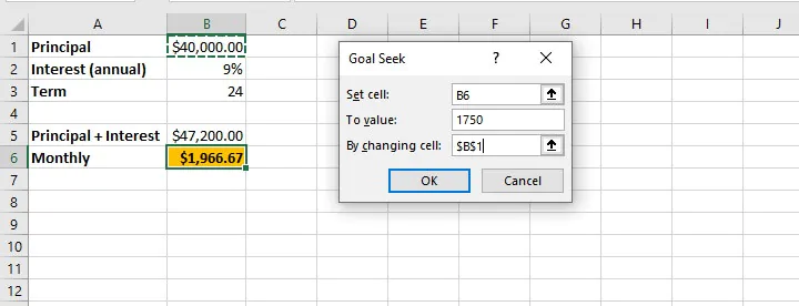
In the example above, cell B5 is dependent on the variables in cells B1, B2, and B3. Cell B6 is dependent on cells B3 and B5. Therefore, if we determine that the monthly repayment amount quoted is higher than desired, we can use Goal Seek to set the monthly amount to $1750. Excel can work backwards to change either cell B1, B2, or B3 to reach that goal.
Practically speaking, we may not have much control over the interest rate, so it is more likely that we have the option of adjusting the amount we borrow, or the repayment period.
Our first inclination may be to find out how much we will be able to borrow if we pay $1750 per month and all other variables remain the same. Excel will change the principal (B1) based on the number we enter as the new value for cell B6.
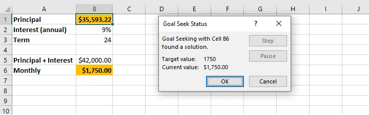
 Assuming that the interest amount (9%) and loan period (24 months) remain the same, the new principal amount is calculated and displayed in cell B1 if a valid solution exists.
 Points to note:
- The cell chosen in the “Set cell” field must be a cell containing a formula.
- The cell chosen in the “By changing cell” field must be a cell containing a constant.
- Once “OK” is selected from the Goal Seek Status window, the values on the worksheet are adjusted and are only retrievable by selecting the ‘Undo’ command (Ctrl+Z Windows shortcut/Cmd+Z Mac shortcut).
Scenario Manager
Another what if analysis tool is the Scenario Manager. This option is somewhat more advanced than Goal Seek in that it allows the adjustment of multiple variables at the same time.
 Some other noticeable differences between Goal Seek and Scenario Manager are listed below:
- The Scenario Manager allows the creation of an unlimited number of possible scenarios by changing up to 32 variables at a time.
- Each scenario can be saved for comparative purposes.
- Scenarios may be named and edited, and a brief description provided.
- Only constant values should be changed within the Scenario Manager — cells with formulas should not be manually adjusted.
If we continue our bank loan example, we can determine our model’s sensitivity to change by adjusting any or all of the values in cell B1, B2, or B3.
Best practice
As a best practice, the original worksheet data should be saved as a scenario so that you can revert to it after all the experiments have been completed.
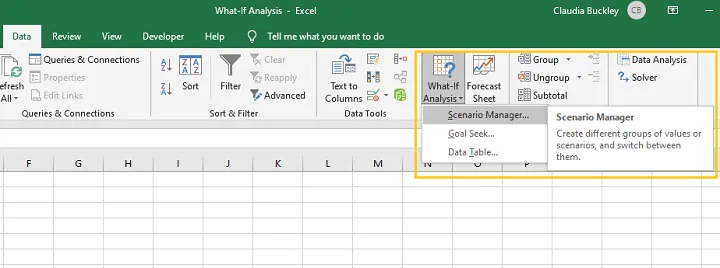
Step 1 — Click ‘What If Analysis’ from the Data tab and select Scenario Manager.
Step 2 — Click ‘Add’ from the Scenario Manager pop-up window.
Step 3 — Name this scenario “Original” and enter the cell references of all cells with constant values that you may consider changing in other scenarios (maximum 32 cells). Click OK.
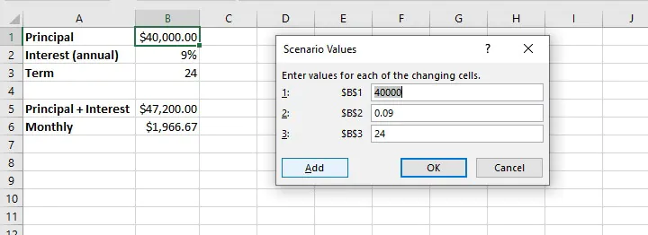
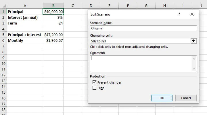 Step 4 — For the “Original” scenario, do not adjust any values in the ‘Scenario Values’ window.
 Step 5 — Click ‘Add’ to create your first experimental scenario.
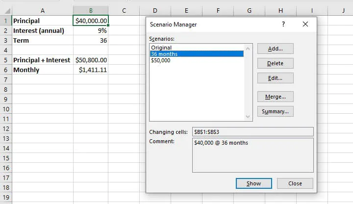
Creating experimental scenarios
When creating an experimental scenario, give the scenario a descriptive name from the ‘Add Scenario’ pop-up window. The changing cells will be the same as the ones referenced in your ‘Original’ scenario.
Even if you will not be adjusting all the values in those cells, it is highly recommended that they remain referenced in the ‘changing cells’ field. You may place additional details about the experimental scenario in the ‘Comment’ field (see below).
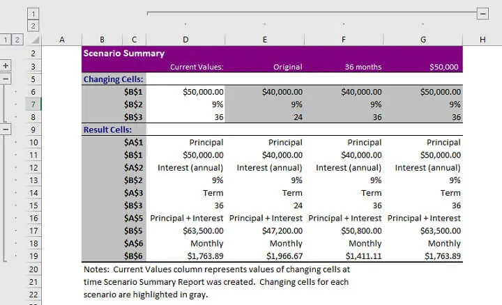
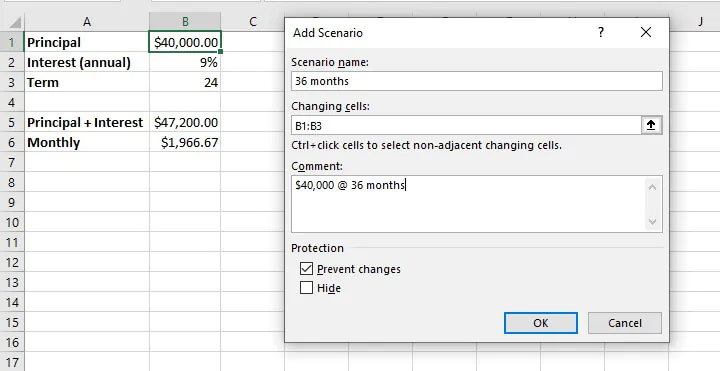 As illustrated above, our experimental scenario is given the name “36 months” and refers to cells B1 to B3 as changing cells. An additional comment indicates that this scenario is to determine the effect of borrowing $40,000 over a 36-month period.
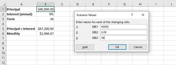
In the ‘Scenario Values’ window, each changing cell is displayed as a field where we can manipulate the constant value so as to affect the outcome of the dependent cells — in our case, cells B5 and B6. As described in our scenario name and comments, we only adjust cell B3 by changing the value to 36.
To add another scenario at this point, select ‘Add’. If not, click OK.
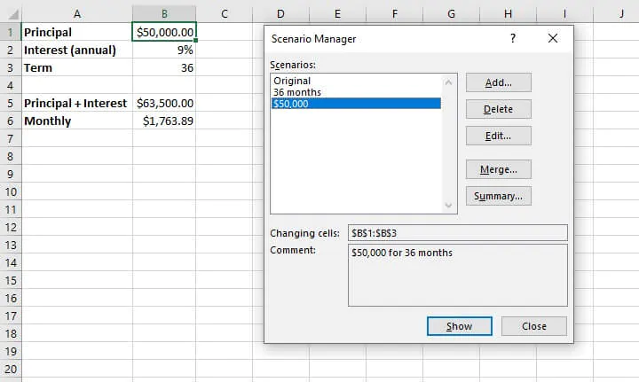
Adjust multiple variables
To experiment with adjusting multiple variables within one scenario, the steps are the same as above, with the exception that the desired changes would be made in the Scenario Values window.
For example, to get Excel to perform a what if analysis on borrowing $50,000 over a 36-month period in the above situation at the same rate of interest, we would simply adjust the fields referencing those variables after creating a new scenario. Excel’s Scenario Manager can handle an unlimited number of scenarios created in this same way.
A list of created scenarios can be viewed by clicking OK from the Scenario Values window, or by selecting Scenario Manager from the What If Analysis dropdown menu.
 To see the outcome of each adjustment on the output cell(s), either double click on a scenario name, or highlight a name and click Show.
Scenario summary
Scenarios that have been created may also be compared side by side with the creation of a Scenario summary worksheet, which is generated by selecting ‘Summary’ from the Scenario Manager window.
There are two report types available — Scenario summary and Scenario PivotTable report. Result cells are the cells that will be displayed in the summary. Ideally, these should include all cells which were adjusted as well as result cells. It’s also a good idea to select cells that contain header names so that these are clearly displayed in the summary.
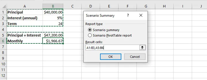 Choosing the ‘Scenario summary’ option will create a new sheet within the workbook that displays each scenario in columnar format. Changing Cells are highlighted in gray, and Result Cells are displayed under Changing Cells.
 Note that if named ranges were created for Changing or Result Cells, range names will be displayed instead of cell references.
Selecting the Scenario PivotTable report type will create a pivot table report in a new worksheet. Learn more about pivot tables from our Resource Library.
Using data tables for what if analysis
The third what if analysis tool from the Forecast command group is the Data Table. Data tables allow the adjustment of only one or two variables within a dataset, but each variable can have an unlimited number of possible values. Data tables are designed for side-by-side comparisons in a way that makes them easier to read than scenarios, once they are set up correctly.
Data tables are under-utilized, but are not as scary as they may seem.
One-variable data tables
If the only variable to be considered in our loan example were the amount being borrowed, we could set up a one-variable data table.
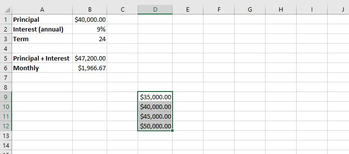
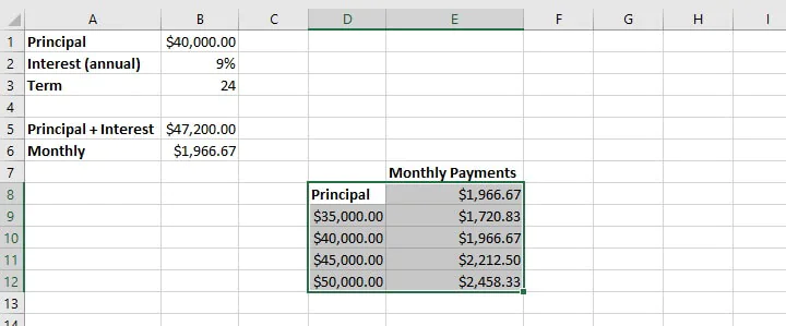
Step 1 — make a list of all possible principal loan amounts. The list may be by column or row. In our example, we will enter a column list in the range D9 to D12.
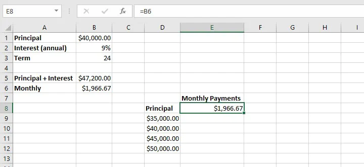
 Step 2 — In an adjacent column, enter the formula which was used to arrive at the original outcome. In this case, we can simply type =B6 in cell E8. This links our new data table to the original variables.
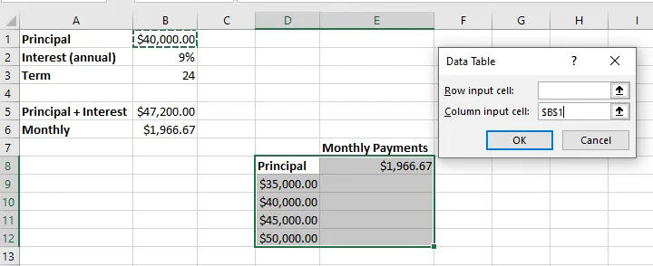
 Step 3 — Select the entire data table range, including the list of variable values, the formula, and blank cells.
Step 4 — From the What If Analysis dropdown menu, select Data Table.
Step 5 — In the column input cell field (since we entered our variables in column format), enter the cell reference that was used to calculate the result in the original dataset. In the above example, this would be cell B1 since this is the variable we have adjusted. No value is entered in the ‘Row input cell’ field in this instance since this is a one-variable data table.
 Step 6 — Select OK. The result is a list of outcomes created by adjusting the one variable in cell B1, assuming that all other variables remain constant.
 To create a row-oriented data table, the variables would be listed horizontally, and the row input cell would be used in the Data Table window instead of the column input cell.
Two-variable data tables
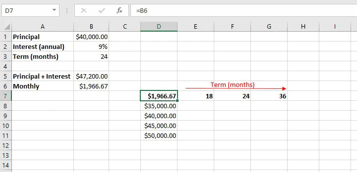
When creating a two-variable data table, one set of values is listed horizontally and the other set is listed vertically. In our example, we will add the loan period (term) as our second variable, displayed horizontally.
In this case, the formula which was used to arrive at the original outcome must be replicated above the vertical list of variables. As shown below, we type =B6 in cell D7. This links our new data table to the original variables.
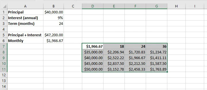
 As before, highlight the entire data table range and select Data Table from the What If Analysis menu. The row input cell is the cell reference (B3) that corresponds to the horizontal variables from the original dataset, while the column input cell (B1) corresponds to the vertical variables.
When we select OK, Excel returns a matrix that can be used to compare the outcome of different changes to our original scenario. It may be necessary to adjust the output cells to the appropriate number format for your data type (in the case of the above example, currency).
Summary
Now that you’ve taken the time to demystify how to do a what if analysis in Excel by using these three main tools, why not experiment with using them in different settings — like budget management, profit margin percentages, project completion targets, and the like?
Once you get the hang of these, you’ll want to check out our resource center and take our Basic and Advanced Excel course to become a real pro!
Ready to become a certified Excel ninja?
Start learning for free with GoSkills courses
Start free trial