
If you know the result that you want from a formula, but are not sure what input value the formula needs to get that result, use the Goal Seek feature. For example, suppose that you need to borrow some money. You know how much money you want, how long you want to take to pay off the loan, and how much you can afford to pay each month. You can use Goal Seek to determine what interest rate you will need to secure in order to meet your loan goal.
If you know the result that you want from a formula, but are not sure what input value the formula needs to get that result, use the Goal Seek feature. For example, suppose that you need to borrow some money. You know how much money you want, how long you want to take to pay off the loan, and how much you can afford to pay each month. You can use Goal Seek to determine what interest rate you will need to secure in order to meet your loan goal.
Note: Goal Seek works only with one variable input value. If you want to accept more than one input value; for example, both the loan amount and the monthly payment amount for a loan, you use the Solver add-in. For more information, see Define and solve a problem by using Solver.
Step-by-step with an example
Let’s look at the preceding example, step-by-step.
Because you want to calculate the loan interest rate needed to meet your goal, you use the PMT function. The PMT function calculates a monthly payment amount. In this example, the monthly payment amount is the goal that you seek.
Prepare the worksheet
-
Open a new, blank worksheet.
-
First, add some labels in the first column to make it easier to read the worksheet.
-
In cell A1, type Loan Amount.
-
In cell A2, type Term in Months.
-
In cell A3, type Interest Rate.
-
In cell A4, type Payment.
-
-
Next, add the values that you know.
-
In cell B1, type 100000. This is the amount that you want to borrow.
-
In cell B2, type 180. This is the number of months that you want to pay off the loan.
Note: Although you know the payment amount that you want, you do not enter it as a value, because the payment amount is a result of the formula. Instead, you add the formula to the worksheet and specify the payment value at a later step, when you use Goal Seek.
-
-
Next, add the formula for which you have a goal. For the example, use the PMT function:
-
In cell B4, type =PMT(B3/12,B2,B1). This formula calculates the payment amount. In this example, you want to pay $900 each month. You don’t enter that amount here, because you want to use Goal Seek to determine the interest rate, and Goal Seek requires that you start with a formula.
The formula refers to cells B1 and B2, which contain values that you specified in preceding steps. The formula also refers to cell B3, which is where you will specify that Goal Seek put the interest rate. The formula divides the value in B3 by 12 because you specified a monthly payment, and the PMT function assumes an annual interest rate.
Because there is no value in cell B3, Excel assumes a 0% interest rate and, using the values in the example, returns a payment of $555.56. You can ignore that value for now.
-
Use Goal Seek to determine the interest rate
-
On the Data tab, in the Data Tools group, click What-If Analysis, and then click Goal Seek.
-
In the Set cell box, enter the reference for the cell that contains the formula that you want to resolve. In the example, this reference is cell B4.
-
In the To value box, type the formula result that you want. In the example, this is -900. Note that this number is negative because it represents a payment.
-
In the By changing cell box, enter the reference for the cell that contains the value that you want to adjust. In the example, this reference is cell B3.
Note: The cell that Goal Seek changes must be referenced by the formula in the cell that you specified in the Set cell box.
-
Click OK.
Goal Seek runs and produces a result, as shown in the following illustration.

Cells B1, B2, and B3 are the values for the loan amount, term length, and interest rate.
Cell B4 displays the result of the formula =PMT(B3/12,B2,B1).
-
Finally, format the target cell (B3) so that it displays the result as a percentage.
-
On the Home tab, in the Number group, click Percentage.
-
Click Increase Decimal or Decrease Decimal to set the number of decimal places.
-

If you know the result that you want from a formula, but are not sure what input value the formula needs to get that result, use the Goal Seek feature. For example, suppose that you need to borrow some money. You know how much money you want, how long you want to take to pay off the loan, and how much you can afford to pay each month. You can use Goal Seek to determine what interest rate you will need to secure in order to meet your loan goal.
Note: Goal Seek works only with one variable input value. If you want to accept more than one input value, for example, both the loan amount and the monthly payment amount for a loan, use the Solver add-in. For more information, see Define and solve a problem by using Solver.
Step-by-step with an example
Let’s look at the preceding example, step-by-step.
Because you want to calculate the loan interest rate needed to meet your goal, you use the PMT function. The PMT function calculates a monthly payment amount. In this example, the monthly payment amount is the goal that you seek.
Prepare the worksheet
-
Open a new, blank worksheet.
-
First, add some labels in the first column to make it easier to read the worksheet.
-
In cell A1, type Loan Amount.
-
In cell A2, type Term in Months.
-
In cell A3, type Interest Rate.
-
In cell A4, type Payment.
-
-
Next, add the values that you know.
-
In cell B1, type 100000. This is the amount that you want to borrow.
-
In cell B2, type 180. This is the number of months that you want to pay off the loan.
Note: Although you know the payment amount that you want, you do not enter it as a value, because the payment amount is a result of the formula. Instead, you add the formula to the worksheet and specify the payment value at a later step, when you use Goal Seek.
-
-
Next, add the formula for which you have a goal. For the example, use the PMT function:
-
In cell B4, type =PMT(B3/12,B2,B1). This formula calculates the payment amount. In this example, you want to pay $900 each month. You don’t enter that amount here, because you want to use Goal Seek to determine the interest rate, and Goal Seek requires that you start with a formula.
The formula refers to cells B1 and B2, which contain values that you specified in preceding steps. The formula also refers to cell B3, which is where you will specify that Goal Seek put the interest rate. The formula divides the value in B3 by 12 because you specified a monthly payment, and the PMT function assumes an annual interest rate.
Because there is no value in cell B3, Excel assumes a 0% interest rate and, using the values in the example, returns a payment of $555.56. You can ignore that value for now.
-
Use Goal Seek to determine the interest rate
-
Do one of the following:
In Excel 2016 for Mac: On the Data tab, click What-If Analysis, and then click Goal Seek.
In Excel for Mac 2011: On the Data tab, in the Data Tools group, click What-If Analysis, and then click Goal Seek.
-
In the Set cell box, enter the reference for the cell that contains the formula that you want to resolve. In the example, this reference is cell B4.
-
In the To value box, type the formula result that you want. In the example, this is -900. Note that this number is negative because it represents a payment.
-
In the By changing cell box, enter the reference for the cell that contains the value that you want to adjust. In the example, this reference is cell B3.
Note: The cell that Goal Seek changes must be referenced by the formula in the cell that you specified in the Set cell box.
-
Click OK.
Goal Seek runs and produces a result, as shown in the following illustration.
-
Finally, format the target cell (B3) so that it displays the result as a percentage. Follow one of these steps:
-
In Excel 2016 for Mac: On the Home tab, click Increase Decimal
or Decrease Decimal . -
In Excel for Mac 2011: On the Home tab, under Number group, click Increase Decimal
or Decrease Decimal to set the number of decimal places.
-
 or Decrease Decimal
  .
. or Decrease Decimal
  to set the number of decimal places.
What is Goal Seek in Excel?
The Goal Seek in excel is a “what-if-analysis” tool that calculates the value of the input cell (variable) with respect to the desired outcome. In other words, the tool helps answer the question, “what should be the value of the input in order to attain the given output?”
For example, the cost price of a product is $15 and the business wants to earn revenue of $50,000. The Goal Seek function can determine the number of units of the product to be sold to achieve the given target of $50,000.
The Goal Seek changes the variable (cause) to study the variations in the result (effect). It shows the impact of change in one value on the other value. This is why it is helpful in cause and effect analysis.
Goal seek function in excel is used in financial modeling and forecasting scenarios.
Table of contents
- What is Goal Seek in Excel?
- Goal Seek Parameters
- How to use Goal Seek in Excel?
- Example #1
- Example #2
- Example #3
- The Rules Governing the Parameters
- Frequently Asked Questions
- Recommended Articles
Goal Seek Parameters
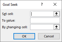
The parameters to be specified in the “Goal Seek” dialog box are stated as follows:
- Set cell–In this box, enter the cell reference of the formula to be resolved. This is the target cell or the formula cell.
- To value–In this box, enter the desired output to be achieved. This is the value of the “set cell” to be attained.
- By changing cell–In this box, enter the reference of the input cell (variable) to be adjusted. This is the cell we want to change in order to impact the “set cell.”
Note: At a given time, Goal Seek works with only one variable input. For working with multiple input values, use the solver in Excel.
You are free to use this image on your website, templates, etc, Please provide us with an attribution linkArticle Link to be Hyperlinked
For eg:
Source: Goal Seek in Excel (wallstreetmojo.com)
How to use Goal Seek in Excel?
Example #1
You can download this Goal Seek Excel Template here – Goal Seek Excel Template
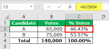
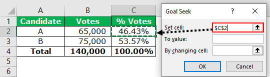
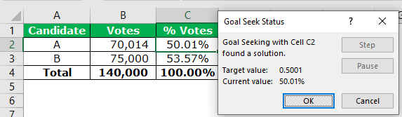
The following table shows the votes received by the two candidates, A and B, who contested in an election. In the present situation, candidate B is leading by 10,000 votes. It is given that to win the election, 50.01% votes are required.
We want to change the voting percentage (column C) of candidate A in such a way that he wins the election. Calculate the total number of votes required by candidate A to win.

Let us calculate the present voting percentage for both the candidates. This is done by dividing the individual votes received by the total votes.
Candidate A has won 46.43% of the total votes. Therefore, he needs only 3.67% votes to win the election.
The steps to use Goal Seek in excel are stated as follows:
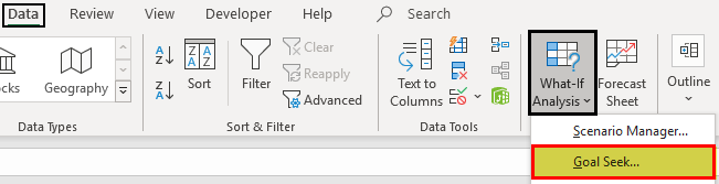
- In the Data tab, click “Goal Seek” from the “what-if-analysis” drop-down.

- The “Goal Seek” excel window appears as shown in the following image.

- Enter $C$2 in the “set cell” box. This is because C2 is the target cell.

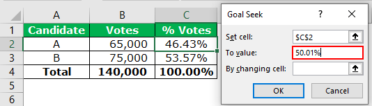
- Enter 50.01% in the “to value” box. This is the value of the “set cell” that we want to obtain. In other words, the “set cell” should change to the target value of 50.01%.

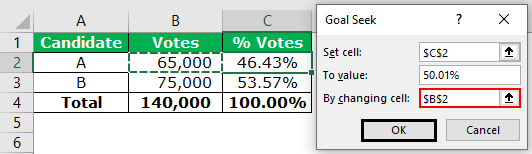
- Enter $B$2 in the “by changing cell” box. This is the cell we want to change to impact the “set cell” C2. Since all the parameters are set, click “Ok” to get the result.

- The output is shown in the following image. Candidate A should secure 70,014 votes to win the election. With 70,014 votes, the voting percentage of candidate A will become 50.01%. Click “Ok” to apply the changes.

The total number of votes and the voting percentage of candidate A has changed. Consequently, the votes and the voting percentage of candidate B also changes.
The votes of candidate B are calculated by subtracting 70,014 from 140,000. The final output is displayed in the following image. Hence, candidate A wins the election.


Example #2
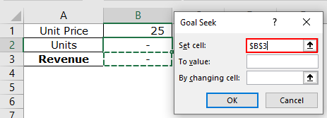
Mr. A opens a retail shop and sells goods at an average selling price of $25 per unit. To meet his operating expenses, he wants to generate monthly revenue of $250,000.
We want to calculate the quantity of the goods Mr. A should sell to earn the given revenue.
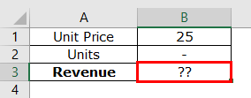
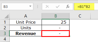
Step 1: In cell B3, apply the formula unit priceUnit Price is a measurement used for indicating the price of particular goods or services to be exchanged with customers or consumers for money. It includes fixed costs, variable costs, overheads, direct labour, and a profit margin for the organization.read more*units (B1*B2).
Step 2: In the Data tab, click “Goal Seek” from the “what-if-analysis” drop-down. The “Goal Seek” window appears as shown in the following image.
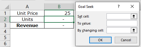
Step 3: Enter $B$3 in the “set cell” box. The target cell is the revenue cell B3.
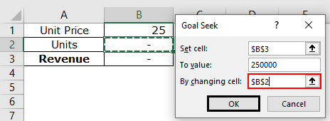
Step 4: Enter 250000 in the “to value” box. This is the value of the “set cell” to be achieved.

Step 5: Enter $B$2 in the “by changing cell.” The quantity has to be calculated in cell B2. So, this is the cell that has to be adjusted to achieve the given revenue. Click “Ok.”
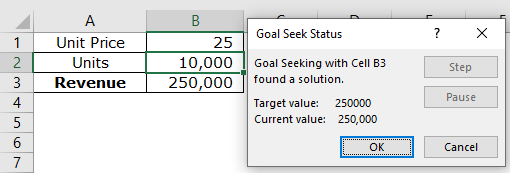
Step 6: The output is displayed in the following image. Hence, Mr. A needs to sell 10,000 units of goods to generate revenue of $250,000. Click “Ok” to apply the changes.
Example #3
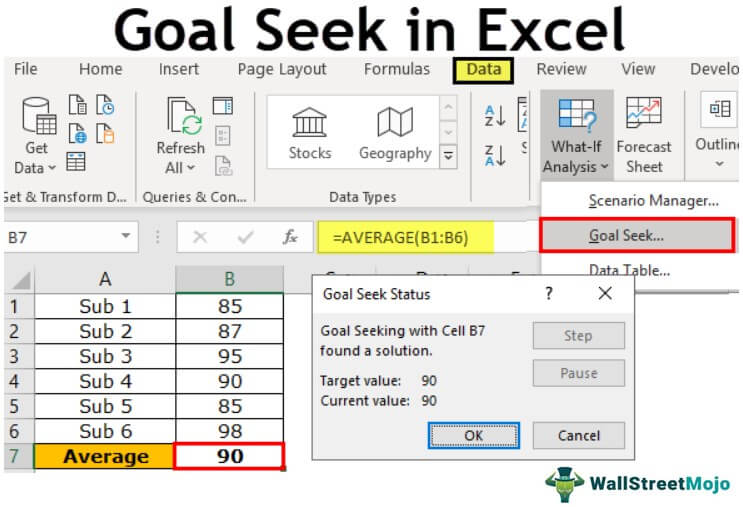
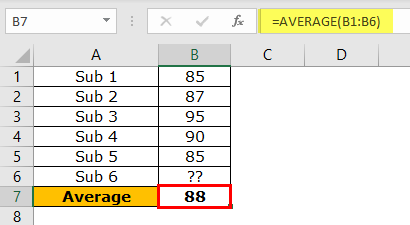
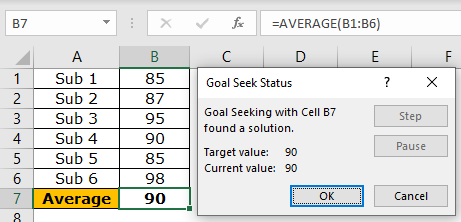
The following table shows the marks obtained (in percentage) by a student in five subjects. Her present average grade is 88%. Since there are six subjects in the class, she is yet to appear for the last examination.
The student is targeting the overall average of 90% from all the six subjects. We want to calculate the marks she should score in the remaining subject to secure the given average.
Step 1: Open the “Goal Seek” window from the Data tab.
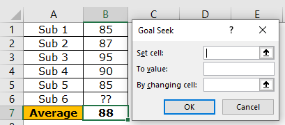
Step 2: Enter $B$7 as the “set cell.” The target cell is the average cell B7.
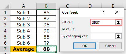
Step 3: Enter “90” in the “to value” box. This is the value we want to attain.
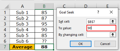
Step 4: Enter $B$6 in the “by changing cell” box. This is the value that has to be adjusted. Click “Ok.”
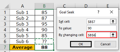
Step 5: The output is displayed in the following image. Hence, the student should score 98% in “subject 6” to get an overall average of 90%. Click “Ok” to apply the changes.
Likewise, the Goal Seek helps identify the exact input that should be adjusted to reach the desired result.
The Rules Governing the Parameters
- The “set cell” should always contain a formula.
- The formula of the “set cell” should depend, whether directly or indirectly, on the “by changing cell.” This is necessary to study the impact on the “set cell.”
- The “by changing cell” should not contain any special characters.
Frequently Asked Questions
Define the Goal Seek in Excel.
The Goal Seek in excel calculates the input value (variable) based on a given output. Being a what-if-analysis tool, the Goal Seek is used when there is a need to study the impact of a change in one value on the other.
The Goal Seek is used in scenario analysis, cause and effect situations, break-even model, sensitivity analysis, and so on. The parameters used in the Goal Seek excel tool are listed as follows:
• “Set cell”–This is the reference of the formula cell.
• “To value” –This is the desired or targeted value to be achieved.
• “By changing cell” –This is the cell reference of the variable to be changed for attaining the desired value.
The Goal Seek works with one input at a given time.
What is Goal Seek used for in Excel?
The Goal Seek in excel is used in the following situations:
• To calculate the input (unknown) for a given output (known)
• To analyze the impact of a change in the input (variable) on the output (set cell)
• To perform what-if-analysis, i.e., explore the various outcomes if different values are used for the input
• To return the closest value (approximate) in case a solution to the problem is not found
Note: The formula used in the Goal Seek analysis remains the same throughout. The input values entered in the “by changing cell” box are changed to study the effect on the output.
How does the Goal Seek work in Excel?
The Goal Seek does backward calculations. It begins from the output that is known and returns the exact input. This input is a requisite for reaching the given output.
The steps showing the working of Goal Seek are listed as follows:
1. Enter data in Excel on which calculations using Goal Seek are to be performed.
2. Click “Goal Seek” from the “what-if-analysis” drop-down in the Data tab.
3. Enter the parameters in the tool.
a. Type the cell reference for the input and the output.
b. Type the target value to be achieved.
4. Click “Ok” to proceed.
5. In the “Goal Seek status” box, click “Ok” to apply the changes to the worksheet.
Note: The initial values can be restored by pressing the “undo” shortcut (Ctrl+Z).
Recommended Articles
This has been a guide to Goal Seek in Excel. Here we learn how to use Goal Seek function in Excel along with step by step examples and a downloadable template. You may learn more about Excel from the following articles –
- Evaluate Formula in ExcelThe Evaluate formula in Excel is used to analyze and understand any fundamental Excel formula such as SUM, COUNT, COUNTA, and AVERAGE. For this, you may use the F9 key to break down the formula and evaluate it step by step, or you may use the “Evaluate” tool.read more
- Create a Data Table in ExcelA data table in excel is a type of what-if analysis tool that allows you to compare variables and see how they impact the result and overall data. It can be found under the data tab in the what-if analysis section.read more
- One Variable Excel Data TableOne variable data table in excel means changing one variable with multiple options and getting the results for multiple scenarios. The data inputs in one variable data table are either in a single column or across a row.read more
- Excel Scenario ManagerScenario Manager is a what-if analysis tool that works with many scenarios that are supplied to it. It uses a set of ranges that have an effect on a certain output and can be used to generate different scenarios such as bad and medium depending on the values.read more
- Excel Shortcut Paste ValuesPasting values is a common procedure that allows us to eliminate any formatting and formulas from the copied cell and paste them into the pasted cell. «Alt + E + S + V» is the shortcut key for pasting values.read more

Очень полезной функцией в программе Microsoft Excel является Подбор параметра. Но, далеко не каждый пользователь знает о возможностях данного инструмента. С его помощью, можно подобрать исходное значение, отталкиваясь от конечного результата, которого нужно достичь. Давайте выясним, как можно использовать функцию подбора параметра в Microsoft Excel.
Суть функции
Если упрощенно говорить о сути функции Подбор параметра, то она заключается в том, что пользователь, может вычислить необходимые исходные данные для достижения конкретного результата. Эта функция похожа на инструмент Поиск решения, но является более упрощенным вариантом. Её можно использовать только в одиночных формулах, то есть для вычисления в каждой отдельной ячейке нужно запускать всякий раз данный инструмент заново. Кроме того, функция подбора параметра может оперировать только одним вводным, и одним искомым значением, что говорит о ней, как об инструменте с ограниченным функционалом.
Применение функции на практике
Для того, чтобы понять, как работает данная функция, лучше всего объяснить её суть на практическом примере. Мы будем объяснять работу инструмента на примере программы Microsoft Excel 2010, но алгоритм действий практически идентичен и в более поздних версиях этой программы, и в версии 2007 года.
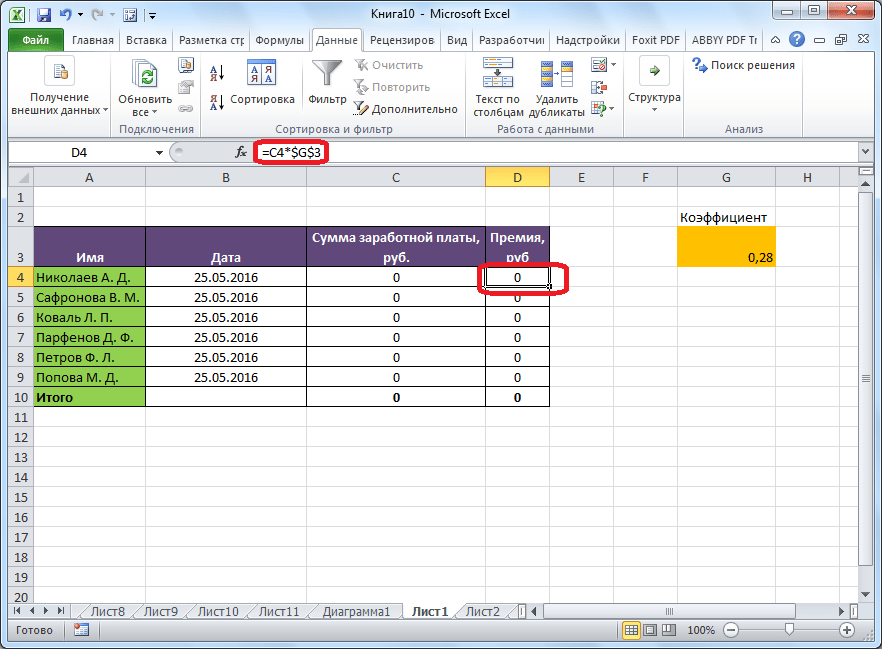
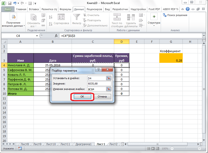
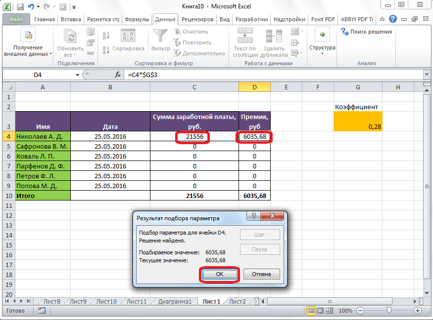
Имеем таблицу выплат заработной платы и премии работникам предприятия. Известны только премии работников. Например, премия одного из них — Николаева А. Д, составляет 6035,68 рублей. Также, известно, что премия рассчитывается путем умножения заработной платы на коэффициент 0,28. Нам предстоит найти заработную плату работников.
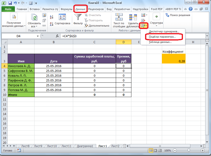
Для того, чтобы запустить функцию, находясь во вкладке «Данные», жмем на кнопку «Анализ «что если»», которая расположена в блоке инструментов «Работа с данными» на ленте. Появляется меню, в котором нужно выбрать пункт «Подбор параметра…».
После этого, открывается окно подбора параметра. В поле «Установить в ячейке» нужно указать ее адрес, содержащей известные нам конечные данные, под которые мы будем подгонять расчет. В данном случае, это ячейка, где установлена премия работника Николаева. Адрес можно указать вручную, вбив его координаты в соответствующее поле. Если вы затрудняетесь, это сделать, или считаете неудобным, то просто кликните по нужной ячейке, и адрес будет вписан в поле.
В поле «Значение» требуется указать конкретное значение премии. В нашем случае, это будет 6035,68. В поле «Изменяя значения ячейки» вписываем ее адрес, содержащей исходные данные, которые нам нужно рассчитать, то есть сумму зарплаты работника. Это можно сделать теми же способами, о которых мы говорили выше: вбить координаты вручную, или кликнуть по соответствующей ячейке.
Когда все данные окна параметров заполнены, жмем на кнопку «OK».
После этого, совершается расчет, и в ячейки вписываются подобранные значения, о чем сообщает специальное информационное окно.
Подобную операцию можно проделать и для других строк таблицы, если известна величина премии остальных сотрудников предприятия.

Решение уравнений
Кроме того, хотя это и не является профильной возможностью данной функции, её можно использовать для решения уравнений. Правда, инструмент подбора параметра можно с успехом использовать только относительно уравнений с одним неизвестным.
Допустим, имеем уравнение: 15x+18x=46. Записываем его левую часть, как формулу, в одну из ячеек. Как и для любой формулы в Экселе, перед уравнением ставим знак «=». Но, при этом, вместо знака x устанавливаем адрес ячейки, куда будет выводиться результат искомого значения.
В нашем случае, формулу мы запишем в C2, а искомое значение будет выводиться в B2. Таким образом, запись в ячейке C2 будет иметь следующий вид: «=15*B2+18*B2».

Запускаем функцию тем же способом, как было описано выше, то есть, нажав на кнопку «Анализ «что если»» на ленте», и перейдя по пункту «Подбор параметра…».

В открывшемся окне подбора параметра, в поле «Установить в ячейке» указываем адрес, по которому мы записали уравнение (C2). В поле «Значение» вписываем число 45, так как мы помним, что уравнение выглядит следующим образом: 15x+18x=46. В поле «Изменяя значения ячейки» мы указываем адрес, куда будет выводиться значение x, то есть, собственно, решение уравнения (B2). После того, как мы ввели эти данные, жмем на кнопку «OK».

Как видим, программа Microsoft Excel успешно решила уравнение. Значение x будет равно 1,39 в периоде.

Изучив инструмент Подбор параметра, мы выяснили, что это довольно простая, но вместе с тем полезная и удобная функция для поиска неизвестного числа. Её можно использовать как для табличных вычислений, так и для решения уравнений с одним неизвестным. Вместе с тем, по функционалу она уступает более мощному инструменту Поиск решения.
Goal Seek Example 1 | Goal Seek Example 2 | Goal Seek Precision | More about Goal Seek
If you know the result you want from a formula, use Goal Seek in Excel to find the input value that produces this formula result.
Goal Seek Example 1
Use Goal Seek in Excel to find the grade on the fourth exam that produces a final grade of 70.
1. The formula in cell B7 calculates the final grade.

2. The grade on the fourth exam in cell B5 is the input cell.

3. On the Data tab, in the Forecast group, click What-If Analysis.

4. Click Goal Seek.

The Goal Seek dialog box appears.
5. Select cell B7.
6. Click in the ‘To value’ box and type 70.
7. Click in the ‘By changing cell’ box and select cell B5.
8. Click OK.

Result. A grade of 90 on the fourth exam produces a final grade of 70.

Goal Seek Example 2
Use Goal Seek in Excel to find the loan amount that produces a monthly payment of $1500.
1. The formula in cell B5 calculates the monthly payment.

Explanation: the PMT function calculates the payment for a loan. If you’ve never heard of this function before, that’s OK. The higher the loan amount, the higher the monthly payment. Assume, you can only afford $1500 a month. What is your maximum loan amount?
2. The loan amount in cell B3 is the input cell.

3. On the Data tab, in the Forecast group, click What-If Analysis.
4. Click Goal Seek.
The Goal Seek dialog box appears.
5. Select cell B5.
6. Click in the ‘To value’ box and type -1500 (negative, you are paying out money).
7. Click in the ‘By changing cell’ box and select cell B3.
8. Click OK.

Result. A loan amount of $250,187 produces a monthly payment of $1500.

Goal Seek Precision
Goal seek returns approximate solutions. You can change the iteration settings in Excel to find a more precise solution.
1. The formula in cell B1 calculates the square of the value in cell A1.

2. Use goal seek to find the input value that produces a formula result of 25.

Result. Excel returns an approximate solution.

3. On the File tab, click Options, Formulas.
4. Under Calculation options, decrease the Maximum Change value by inserting some zeros. The default value is 0.001.

5. Click OK.
6. Use Goal Seek again. Excel returns a more precise solution.

More about Goal Seek
There are many problems Goal Seek can’t solve. Goal Seek requires a single input cell and a single output (formula) cell. Use the Solver in Excel to solve problems with multiple input cells. Sometimes you need to start with a different input value to find a solution.
1. The formula in cell B1 below produces a result of -0.25.

2. Use Goal Seek to find the input value that produces a formula result of +0.25.

Result. Excel can’t find a solution.

3. Click Cancel.
4. Start with an input value greater than 8.

5. Use Goal Seek again. Excel finds a solution.

Explanation: y = 1 / (x —  is discontinuous at x = 8 (dividing by 0 is not possible). In this example, Goal seek cannot reach one side of the x-axis (x>8) if it starts on the other side of the x-axis (x<8) or vice versa.
The Goal Seek Excel function (often referred to as What-if-Analysis) is a method of solving for a desired output by changing an assumption that drives it. The function essentially uses a trial and error approach to back-solving the problem by plugging in guesses until it arrives at the answer.
Contents
- 1 How does a what if analysis differ from a goal seeking analysis?
- 2 Can you automate Goal Seek in Excel?
- 3 Is solver a what if analysis in Excel?
- 4 How do you use Goal Seek in Excel cell must contain a value?
- 5 What if analysis option contains Goal Seek option True or false?
- 6 How do you use Goal Seek analysis in Excel?
- 7 How do I make goal seek more accurate?
- 8 Can you make goal seek dynamic?
- 9 Which statement best describes what-if goal seeking?
- 10 What are examples of if scenarios?
- 11 What is the use of what if analysis?
- 12 When using the goal seeking function the 3 inputs are?
- 13 Which tab holds the what if analysis option?
- 14 How is what if analysis carried out through scenarios in worksheet?
- 15 What is more elaborate form of Goal Seek?
- 16 What is the difference between solver and goal seek in Excel?
- 17 How do you do a what if analysis data table?
- 18 When using Goal Seek you can find a target result by varying?
- 19 How do I change my Goal Seek iterations?
- 20 How do you increase the number of iterations in Goal Seek?
How does a what if analysis differ from a goal seeking analysis?
A what-if analysis is a process of changing values in (Microsoft Excel) cells to see how these changes will affect formula outcomes on the worksheet. When you are goal seeking, you are performing what-if analysis on a given value, or the output.
Can you automate Goal Seek in Excel?
The only way to automate Goal Seek is using VBA. The easiest way of using VBA is by recording a macro. If you’re not familiar with this concept, a macro is a feature that creates a VBA code.You can make it visible by enabling from Excel Options > Customize Ribbon.
Is solver a what if analysis in Excel?
Solver is a Microsoft Excel add-in program you can use for what-if analysis. Use Solver to find an optimal (maximum or minimum) value for a formula in one cell — called the objective cell — subject to constraints, or limits, on the values of other formula cells on a worksheet.
How do you use Goal Seek in Excel cell must contain a value?
In the Goal Seek dialog box, fill out the criteria for your search:
- Set cell: Select the cell that contains your results formula. (The cell must contain a formula for Goal Seek to work!)
- To value: Type the amount you want the formula to return.
- By changing cell: Select the cell of your unknown variable.
What if analysis option contains Goal Seek option True or false?
Use Goal Seek to determine the interest rate
In the To value box, type the formula result that you want. In the example, this is -900. Note that this number is negative because it represents a payment. In the By changing cell box, enter the reference for the cell that contains the value that you want to adjust.
How do you use Goal Seek analysis in Excel?
How to Use Excel Goal Seek
- Create a spreadsheet in Excel that has your data.
- Click the cell you want to change.
- From the Data tab, select the What if Analysis…
- Select Goal seek… from the drop-down menu.
- In the Goal Seek dialog, enter the new “what if” amount in the To value: text box.
How do I make goal seek more accurate?
To make Goal Seek more accurate, we do the following:
- Select Options from the File tab.
- Choose Formulas.
- On the right of the dialog box under Calculation Options, simply reduce Maximum Change to a very small number (say 0.0000000000001).
Can you make goal seek dynamic?
The goal seek is a wonderful tool in excel. But sometimes you may want to have the goal seek work on a dynamic basis, meaning that you do not want to go to the data menu and then hit the what if analysis and enter the target cell etc.
Which statement best describes what-if goal seeking?
Which statement best describes an Excel What-If Analysis Goal Seeking? Allows you to define output results and then shows what input values are needed to generate that result.
What are examples of if scenarios?
An example of what-if analysis would be to ask: what would happen to my revenue if I charged more for each loaf of bread? In the simple case, where the volume of bread sold doesn’t depend on the price of the bread, the analysis is very easy. An X% rise in the price per loaf will lead to an X% increase in sales.
What is the use of what if analysis?
Overview. What-If Analysis is the process of changing the values in cells to see how those changes will affect the outcome of formulas on the worksheet. Three kinds of What-If Analysis tools come with Excel: Scenarios, Goal Seek, and Data Tables.
When using the goal seeking function the 3 inputs are?
Goal Seek uses the result that you want and calculates one of the values that you need, to achieve it. Goal Seek requires three components: a formula to run values through; a target value to achieve and; a cell that it can change while testing the values. The cell to be changed must be referred to in the formula.
Which tab holds the what if analysis option?
From the Data tab, click the What-If Analysis command, then select Goal Seek from the drop-down menu.
How is what if analysis carried out through scenarios in worksheet?
Scenario Manager is one of the What-if Analysis tools in Excel. Step 1 − Define the set of initial values and identify the input cells that you want to vary, called the changing cells. Step 2 − Create each scenario, name the scenario and enter the value for each changing input cell for that scenario.
What is more elaborate form of Goal Seek?
Solver is a more elaborate form of Goal Seek.
What is the difference between solver and goal seek in Excel?
Goal Seek determines what value needs to be in an input cell to achieve a desired result in a formula cell. Solver determines what values need to be in multiple input cells to achieve a desired result.
How do you do a what if analysis data table?
Do the analysis with the What-If Analysis Tool Data Table
- Select the range of cells that contains the formula and the two sets of values that you want to substitute, i.e. select the range – F2:L13.
- Click the DATA tab on the Ribbon.
- Click What-if Analysis in the Data Tools group.
- Select Data Table from the dropdown list.
When using Goal Seek you can find a target result by varying?
Goal Seek requires a formula that uses the input value to give result in the target value. Then, by varying the input value in the formula, Goal Seek tries to arrive at a solution for the input value. Goal Seek works only with one variable input value.
How do I change my Goal Seek iterations?
Iteration in Excel with Goal Seek
- Open Goal Seek.
- Select the cell that you want to achieve a specific target with in the “set cell” input.
- Enter the target value you want to achieve (“to value”).
- Provide the cell that you want to change to achieve the result, or “by changing cell”.
- Select OK.
How do you increase the number of iterations in Goal Seek?
Whist it should be possible to limit the number of iterations that Goal Seek makes by default (100) through either FIle>Options>Formulas>Maximum Iterations – or a short VBA instruction Application.