
Содержание
- Create a PivotTable to analyze worksheet data
- Analysis of data in excel with examples of reports
- Excel analysis tools
- Summary tables in data analysis
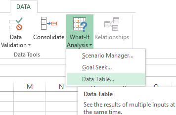
- Analysis «What-if Analysis» in Excel: «Data Table»
- Introduction to What-If Analysis
- Need more help?
Create a PivotTable to analyze worksheet data
A PivotTable is a powerful tool to calculate, summarize, and analyze data that lets you see comparisons, patterns, and trends in your data. PivotTables work a little bit differently depending on what platform you are using to run Excel.


Select the cells you want to create a PivotTable from.
Note: Your data should be organized in columns with a single header row. See the Data format tips and tricks section for more details.
Select Insert > PivotTable.
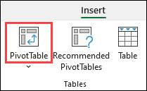
This will create a PivotTable based on an existing table or range.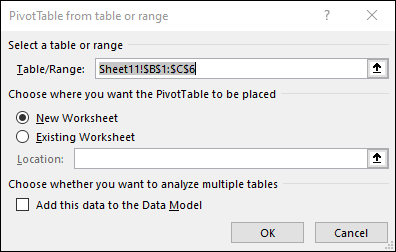
Note: Selecting Add this data to the Data Model will add the table or range being used for this PivotTable into the workbook’s Data Model. Learn more.
Choose where you want the PivotTable report to be placed. Select New Worksheet to place the PivotTable in a new worksheet or Existing Worksheet and select where you want the new PivotTable to appear.
By clicking the down arrow on the button, you can select from other possible sources for your PivotTable. In addition to using an existing table or range, there are three other sources you can select from to populate your PivotTable.
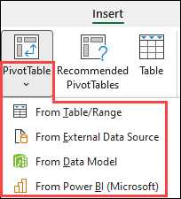
Note: Depending on your organization’s IT settings you might see your organization’s name included in the button. For example, «From Power BI (Microsoft)»
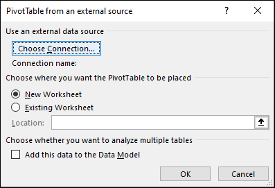
Get from External Data Source
Get from Data Model
Use this option if your workbook contains a Data Model, and you want to create a PivotTable from multiple Tables, enhance the PivotTable with custom measures, or are working with very large datasets. 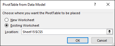
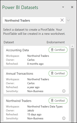
Get from Power BI
Use this option if your organization uses Power BI and you want to discover and connect to endorsed cloud datasets you have access to.
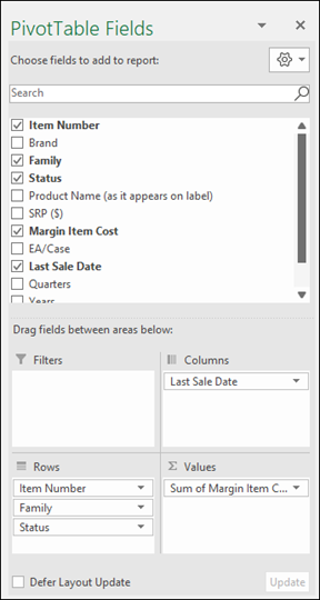
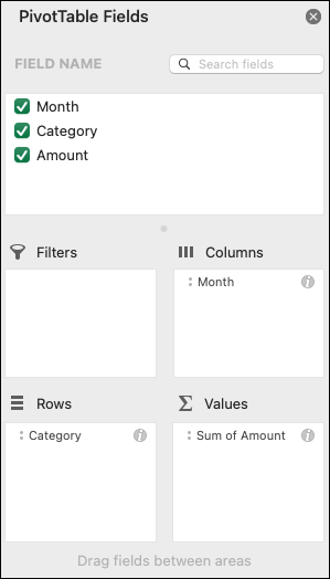
To add a field to your PivotTable, select the field name checkbox in the PivotTables Fields pane.
Note: Selected fields are added to their default areas: non-numeric fields are added to Rows, date and time hierarchies are added to Columns, and numeric fields are added to Values.
To move a field from one area to another, drag the field to the target area.
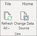
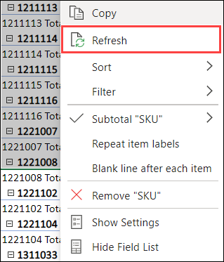
If you add new data to your PivotTable data source, any PivotTables that were built on that data source need to be refreshed. To refresh just one PivotTable you can right-click anywhere in the PivotTable range, then select Refresh. If you have multiple PivotTables, first select any cell in any PivotTable, then on the Ribbon go to PivotTable Analyze > click the arrow under the Refresh button and select Refresh All.
Summarize Values By
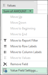
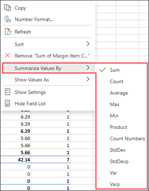
By default, PivotTable fields that are placed in the Values area will be displayed as a SUM. If Excel interprets your data as text, it will be displayed as a COUNT. This is why it’s so important to make sure you don’t mix data types for value fields. You can change the default calculation by first clicking on the arrow to the right of the field name, then select the Value Field Settings option.
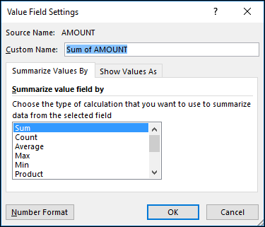
Next, change the calculation in the Summarize Values By section. Note that when you change the calculation method, Excel will automatically append it in the Custom Name section, like «Sum of FieldName», but you can change it. If you click the Number Format button, you can change the number format for the entire field.
Tip: Since the changing the calculation in the Summarize Values By section will change the PivotTable field name, it’s best not to rename your PivotTable fields until you’re done setting up your PivotTable. One trick is to use Find & Replace ( Ctrl+H) > Find what > » Sum of«, then Replace with > leave blank to replace everything at once instead of manually retyping.
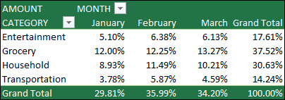
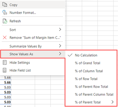
Instead of using a calculation to summarize the data, you can also display it as a percentage of a field. In the following example, we changed our household expense amounts to display as a % of Grand Total instead of the sum of the values.
Once you’ve opened the Value Field Setting dialog, you can make your selections from the Show Values As tab.
Display a value as both a calculation and percentage.
Simply drag the item into the Values section twice, then set the Summarize Values By and Show Values As options for each one.
Источник
Analysis of data in excel with examples of reports
Data analysis in Excel is provided by construction of a table processor. A lot of the program’s resources are suitable for solving this task.
Excel positions itself as the best universal software product in the world for processing analytical information. From a small enterprise to large corporations, managers spend a significant part of their working hours analyzing their businesses activity. Let’s consider the main analytical tools in Excel and examples of their use in practice.
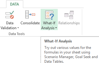
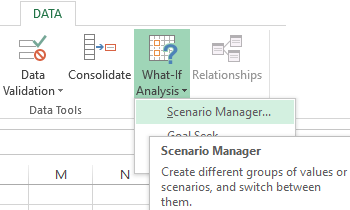
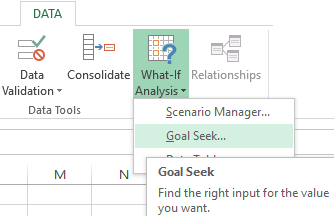
One of the most attractive data analysis is «What-if Analysis». It is located in «DATA» tab.
Analysis tools of «What-if Analysis»:
- “Scenario Manager”. It is used to generate, change and save different sets of input data and the results of calculations for a group of formulas.

- «Goal Seek». It is used when the user knows the result of the formula, but the input information for this result is unknown.
- «Data Table». Used in situations when it is necessary to show the effect of variable values on formulas in the form of a table.
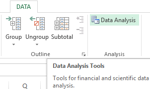
«Data Analysis». This is an Excel add-in. Helps find the best solution for a particular task.
Other tools for analysis:
Analyze data in Excel using built-in functions (mathematical, financial, logical, statistical, etc.).
Summary tables in data analysis
Excel uses summary tables to simplify the viewing, processing and consolidation of data.
The program will treat the entered information as a table, but not as a simple information set. But firstly you should format lists with values according to next steps:
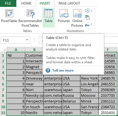
- Go to the «INSERT» tab and click on the «Table» button CTRL+T.
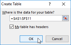
- The «Create Table» dialog box appears.
- Specify the range of data (if it already exist) or the expected range (in which cells the table will be placed).
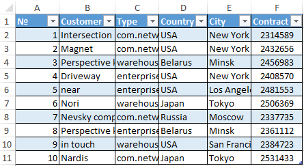
Set the check-mark in the box next to «Table with titles». Press Enter.
The specified default formatting style applies to the specified range.
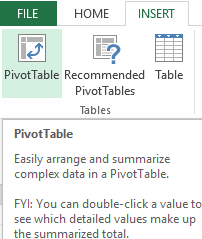
You can compose the report using the «PivotTable».
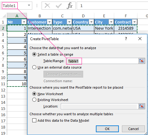
- Activate any of the cells in the values range. We click the button «PivotTable» («INSERT» — «Tables» — «PivotTable»).
- In the dialog box you specify the range and place where to put the summary report (new sheet).
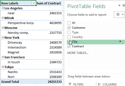
- The «PivotTable Fields» opens. The left side of the sheet is the report image; the right part is the tools for creating the summary report.
- Select the required fields from the list. Determine the values for the names of rows and columns. The report will be built on the left side of the sheet.
Creating a pivot table is already a way for analyzing information. Moreover, the user selects the information he needs at a particular moment for displaying. Then he can use other tools.
Analysis «What-if Analysis» in Excel: «Data Table»
This is a powerful tool for information analysis. Let’s consider the organization of information using the tool «What-if Analysis» — «Data Table».
- data must be in one column or one line;
- the formula refers to one input cell.
The procedure for creating analysis:
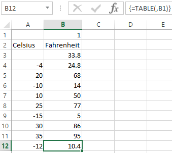
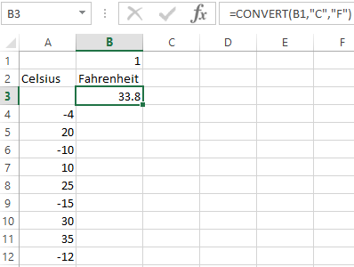
- We enter the input values in a column. Enter the formula in the next column one line higher.
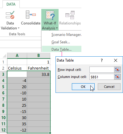
- We select a range of values including a column with input values and a formula A3:B12. Go to the «DATA» tab. Open the «What-if Analysis» tool. We click the «Data Table» button.
- There are two fields in the opened dialog box. Since we create a table with one input we enter the address only in the field «Column input cell:». If the input values are in lines (not in columns), we will enter the cell’s number in the field «Row input cell: » and click OK.
- Download enterprise analysis system
- Download analytical finance table
- Business profitability table
- Cash flow statement
- Example of a point method in financial and economic analytics
When using the features Excel, to analyze the enterprise activity, we use information from the balance sheet and income statement. Each user creates his own form, which reflects the features of the company and important information for decision-making.
Источник
Introduction to What-If Analysis
By using What-If Analysis tools in Excel, you can use several different sets of values in one or more formulas to explore all the various results.
For example, you can do What-If Analysis to build two budgets that each assumes a certain level of revenue. Or, you can specify a result that you want a formula to produce, and then determine what sets of values will produce that result. Excel provides several different tools to help you perform the type of analysis that fits your needs.
Note that this is just an overview of those tools. There are links to help topics for each one specifically.
What-If Analysis is the process of changing the values in cells to see how those changes will affect the outcome of formulas on the worksheet.
Three kinds of What-If Analysis tools come with Excel: Scenarios, Goal Seek, and Data Tables. Scenarios and Data tables take sets of input values and determine possible results. A Data Table works with only one or two variables, but it can accept many different values for those variables. A Scenario can have multiple variables, but it can only accommodate up to 32 values. Goal Seek works differently from Scenarios and Data Tables in that it takes a result and determines possible input values that produce that result.
In addition to these three tools, you can install add-ins that help you perform What-If Analysis, such as the Solver add-in. The Solver add-in is similar to Goal Seek, but it can accommodate more variables. You can also create forecasts by using the fill handle and various commands that are built into Excel.
For more advanced models, you can use the Analysis ToolPak add-in.
A Scenario is a set of values that Excel saves and can substitute automatically in cells on a worksheet. You can create and save different groups of values on a worksheet and then switch to any of these new scenarios to view different results.
For example, suppose you have two budget scenarios: a worst case and a best case. You can use the Scenario Manager to create both scenarios on the same worksheet, and then switch between them. For each scenario, you specify the cells that change and the values to use for that scenario. When you switch between scenarios, the result cell changes to reflect the different changing cell values.
1. Changing cells
1. Changing cells
If several people have specific information in separate workbooks that you want to use in scenarios, you can collect those workbooks and merge their scenarios.
After you have created or gathered all the scenarios that you need, you can create a Scenario Summary Report that incorporates information from those scenarios. A scenario report displays all the scenario information in one table on a new worksheet.
Note: Scenario reports are not automatically recalculated. If you change the values of a scenario, those changes will not show up in an existing summary report. Instead, you must create a new summary report.
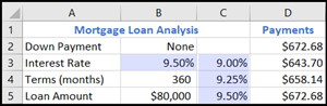
If you know the result that you want from a formula, but you’re not sure what input value the formula requires to get that result, you can use the Goal Seek feature. For example, suppose that you need to borrow some money. You know how much money you want, how long a period you want in which to pay off the loan, and how much you can afford to pay each month. You can use Goal Seek to determine what interest rate you must secure in order to meet your loan goal.

Cells B1, B2, and B3 are the values for the loan amount, term length, and interest rate.
Cell B4 displays the result of the formula =PMT(B3/12,B2,B1).
Note: Goal Seek works with only one variable input value. If you want to determine more than one input value, for example, the loan amount and the monthly payment amount for a loan, you should instead use the Solver add-in. For more information about the Solver add-in, see the section Prepare forecasts and advanced business models, and follow the links in the See Also section.
If you have a formula that uses one or two variables, or multiple formulas that all use one common variable, you can use a Data Table to see all the outcomes in one place. Using Data Tables makes it easy to examine a range of possibilities at a glance. Because you focus on only one or two variables, results are easy to read and share in tabular form. If automatic recalculation is enabled for the workbook, the data in Data Tables immediately recalculates; as a result, you always have fresh data.
Cell B3 contains the input value.
Cells C3, C4, and C5 are values Excel substitutes based on the value entered in B3.
A Data Table cannot accommodate more than two variables. If you want to analyze more than two variables, you can use Scenarios. Although it is limited to only one or two variables, a Data Table can use as many different variable values as you want. A Scenario can have a maximum of 32 different values, but you can create as many scenarios as you want.
If you want to prepare forecasts, you can use Excel to automatically generate future values that are based on existing data, or to automatically generate extrapolated values that are based on linear trend or growth trend calculations.
You can fill in a series of values that fit a simple linear trend or an exponential growth trend by using the fill handle or the Series command. To extend complex and nonlinear data, you can use worksheet functions or the regression analysis tool in the Analysis ToolPak Add-in.
Although Goal Seek can accommodate only one variable, you can project backward for more variables by using the Solver add-in. By using Solver, you can find an optimal value for a formula in one cell—called the target cell—on a worksheet.
Solver works with a group of cells that are related to the formula in the target cell. Solver adjusts the values in the changing cells that you specify—called the adjustable cells—to produce the result that you specify from the target cell formula. You can apply constraints to restrict the values that Solver can use in the model, and the constraints can refer to other cells that affect the target cell formula.
Need more help?
You can always ask an expert in the Excel Tech Community or get support in the Answers community.
Источник
One of the most appealing aspects of Excel is its ability to create dynamic models. A dynamic model uses formulas that instantly recalculate when you change values in cells that are used by the formulas. When you change values in cells in a systematic manner and observe the effects on specific formula cells, you’re performing a type of what-if analysis.
Excel includes many powerful tools to perform complex mathematical calculations, including what-if analysis. This feature can help you experiment and answer questions with your data, even when the data is incomplete.
Excel’s what-if analysis tools:
- Goal Seek
- Scenario Manager
- Data Table
- Solver
PART 1: Goal Seek and Scenario Manager
What is Goal Seek?
When you create a formula or function in Excel, you put various parts together to calculate a result. Goal Seek works in the opposite way: It lets you start with the desired result, and it calculates the input value that will give you that result. We’ll use a few examples to show how to use Goal Seek.
How to Use Excel Goal Seek?
Example 1:
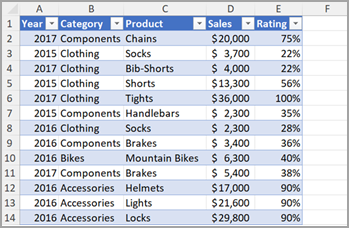
Let’s say you’re enrolled in a class. You currently have a percentage of 15, and you need at least 60% to pass the class. Luckily, you have final exam that might be able to raise your average. You can use Goal Seek to find out how much you have score in final exam to get first class?
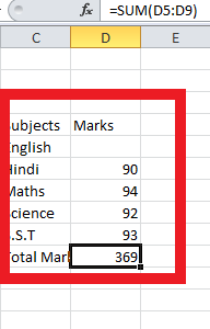
In the image below, you can see that the marks obtained in internal and mid-term exam are 12 and 30. Even though we don’t know what the final exam marks will be, we can go ahead and write a formula or function that calculates the final percentage. In this case, percentage is calculated by applying this formula in cell C8, =SUM(C5:C7)/D8. Once we use Goal Seek, cell C7 will show us the minimum marks we’ll need to make in final exam.

- Select the cell containing the value you want to change. When you use Goal Seek, you’ll need to select a cell that already contains a formula or function. In our example, we’ll select cell C8 because it contains the formula =SUM(C5:C7)/D8.

- Begin by clicking on the Data tab on the Ribbon and locating the What-If Analysis button in the Data Tools Click on the What-If Analysis button and choose Goal Seek from the menu.

- A dialog box will appear with three fields:
- Set cell: This is the cell that will contain the desired result. In our example, cell C8 is already selected.
- To value: This is the desired result. In our example, we’ll enter 60% because we need to earn at least that to pass the class.
- By changing cell: This is the cell where Goal Seek will place its answer. In our example, we’ll select cell C7 because we want to determine the grade we need to earn on the final assignment.
- When you’re done, click OK.

- The dialog box will tell you if Goal Seek was able to find a solution. Click OK.

- The result will appear in the specified cell. In our example, Goal Seek calculated that we will need to score at least 63 marks in final exam to get first class.


Example 2:
Let’s say you need a loan to buy a new car. You already know you want a loan amount of $20,000, a 60-month term—the length of time it takes to pay off the loan—and a payment which is not more than $400 per month. However, you’re not sure yet what the interest rate will be.
In the image below, you can see that Interest Rate is left blank and Payment is $333.33. This is because the payment is being calculated by a specialized function called the PMT (Payment) function, and $333.33 is what the monthly payment would be if there was no interest ($20,000 divided by 60 monthly payments).

Function calculating the monthly paymentIf we typed different values into the empty Interest Rate cell, we could eventually find the value that causes Payment to be $400, and that would be the highest interest rate that we could afford. However, Goal Seek can do this automatically by starting with the result and working backward.
We can use Goal Seek to find the interest rate we’ll need.
- From the Data tab, click the What-If Analysis
- Select Goal Seek.
- A dialog box will appear containing three fields:
- Set cell: This is the cell that will contain the desired result (in this case, the monthly payment). In this example, we will set it to B8 (it doesn’t matter whether it’s an absolute or relative reference).
- To value: This is the desired result. We’ll set it to -400. Because we’re making a payment that will be subtracted from our loan amount, we have to enter the payment as a negative number.
- By changing cell: This is the cell where Goal Seek will place its answer (in this case, the interest rate). We’ll set it to B7.

- When you’re done, click OK. The dialog box will tell you whether Goal Seek was able to find a solution. In this example, the solution is 7%, and it has been placed in cell B4. This tells us that a 7% interest rate will give us a $400-per-month payment on a $20,000 loan that is paid off over five years, or 60 months.


What is Scenario Manager?
A Scenario is a set of values that Excel saves and can substitute automatically in cells on a worksheet. You can create and save different groups of values on a worksheet and then switch to any of these new scenarios to view different results.
For each scenario, you need to give it a unique name. The scenarios can be saved as part of the workbook. You can switch between scenarios to see how the inputs can affect the final output by double clicking on any of the scenarios in the Scenario Manager Dialogue box. Moreover, with the saved Scenarios, Excel can also create a beautiful summary report containing the various sets of inputs and corresponding final outputs to facilitate review.
How to Use Scenario Manager?
Suppose that we are going to sell a book and would like to know how the Sale Units, Price per Unit and Variable Cost per Unit can affect the final profits. Figure below shows how the dataset is constructed. The profit is dependent on Sale Units in Cell C2, Price per Unit in Cell C3 and the Variable Cost per Unit in Cell C5. Therefore, we typed formula “=C2*C3-C4-C2*C5” in Cell C6.

- Go to Data tab and click on What-If Analysis in Data Tools In the drop-down, choose Scenario Manager.

- In the Scenario Manager dialogue box, click on Add.

- In the prompted Add Scenario dialogue box, fill in the required details. Enter a name Worst Case for the Scenario name Add any comment that you wish to into the Comment box. Or you can also leave it blank. As for the Changing cells, fill in the all the reference cells C2, C3, C5 in this case that contain the input values.Please note that the references must be separated by commas. Or, just press CTRL key on your keyboard and select all the cells, one by one, that contain the input values.

- Click OK to open the Scenario Values dialogue box. Fill in the Scenario Values dialog box with the input values that define the worst case, as shown in Figure. Click on OK, the Worst Case scenario will be successfully created. Since we’d like to create another scenario, we click on Add button. After clicking on Add, another Add Scenario dialogue box will appear.

- Use the same approach that we applied when creating Worst Case scenario to build Best Case scenario. The details are shown in following Figure.


- With the same approach, create Most Likely Case scenario. Here Figure represents the details. You can also use the same above approach to creating other scenarios if you have other combination of input values. In this example, we assume that there are only 3 scenarios available.


- Now we click on the OK button in Scenario Values dialogue box. From the Figure, you can see that three scenarios have been successfully created and they are listed in sequence.


How to view different scenarios:
So far, you have saved all of those 3 scenarios in your workbook. Now you can view the result from each of the scenarios by simply double clicking on any of the scenarios. For example, if we double click on Worst Case, the input values in Excel worksheet will change into what have filled for Worst Case and the output value will be calculated automatically based on the formula in cell C6. To view a specific scenario and its corresponding outputs, you can also click on that scenario and then click on the Show button at the bottom. The right part in Figure shows how the Excel worksheet looks like if we click on Best Case scenario and then click on Show.

How to create a summary report:
- I have already told you in the introduction part that Excel can create a summary report based on the saved scenarios. Now let’s see how to make a summary report. Go to Data tab and click on What-If Analysis, then choose Scenario Manager in the drop-down to open Scenario Manager Dialogue box. In the prompted Scenario Manager dialogue box, click on Summary Button.

- After clicking on Summary, a Scenario Summary dialog box appears for you to put Result cells C6 in this case and choose between Scenario summary and Scenario Pivot Table report.

- Figure shows that a Scenario summary report with all of the three scenarios is created with a new tab if you choose Scenario summary in Figure.

- Otherwise, a Scenario Pivot Table report is created with a new tab if you choose Scenario Pivot Table report.


Notes:
- It’s hard to create lots of scenarios with the Scenario Manager because you need to input each individual scenario’s input values. The work will be time-consuming and also expose you to a high risk of making a mistake.
- Suppose that you send a file to several people and ask them to add own scenarios. After you receive all workbooks, you can merge all the scenarios into one workbook. Open each person’s workbook and click Merge button in the Scenario Manager Dialog box in the original workbook. In the Merge Scenarios dialog box, select the workbook containing the scenarios that you want to merge. Do the same things with all of the workbooks. Figure shows you how to choose the workbook in Merge Scenarios dialog box. Click OK. You will return to the previous dialog box, which now displays the scenario names that you merged from the other workbook.

Reference:
- https://www.gcflearnfree.org/excel2010/using-whatif-analysis/1/
- http://stephenlnelson.com/articles/what-if-analysis-scenario-manager-excel/

About M.Hemalatha:
M.Hemalatha is a B.Tech (Telecommunication Engineering). Currently she is working as Analyst Intern with NikhilGuru Consulting Analytics Service LLP (Nikhil Analytics), Bangalore.
What-if analysis is the option available in Data. In what-if analysis, by changing the input value in some cells you can see the effect on output. It tells about the relationship between input values and output values. In this article, we will learn how to use the what-if analysis with data tables effectively.
What is What-if Analysis?
What-if analysis is a procedure in excel in which we work in tabular form data. In the What-if analysis variety of values have been in the cell of the excel sheet to see the result in different ways by not creating different sheets. There are three tools of what-if analysis.
Tools of what-if analysis
There are three tools in what-if analysis:
- Goal seek
- Scenario manager
- Data Table
Goal seek
In goal seek we already know our output value we have to find the correct input value. For example, if a student wants to know his English marks and he knows all the rest of the marks and total marks in all subjects.
Step 1: Write all subjects and their marks in an excel sheet and do the sum by applying the formula sum.
Step 2: Go into the data tab of the Toolbar.

Step 3: Under the Data Table section, Select the What-if analysis.

Step 4: A drop-down appears. Select the Goal Seek.

Step 5: The dialogue box appears in the first column write the name of the cell in which you apply the formula sum. Type D10 in Set cell.

Step 6: In the second column write the value of the target. The target value for this example is 440.

Step 7: In the third column write the name of the cell in which you want to get marks in English. Provide absolute cell reference, i.e. $D$5.

Step 8: Click ok and see the result. The estimated marks for English are 71.

Scenario Manager
In scenario manager, we create different scenarios by proving different input values for the same variable than by comparing scenarios to choose the correct result. For Example, To check the cost of revenue for three different months.
Step 1: Given a data set, for Revenue Cost of Jan, with Expenses and Cost as its columns.

Step 2: Select the numerical value cell and Go to the Data.

Step 3: Under the forecast section, click on the What-if analysis.

Step 4: A drop-down appears. Select the Scenario manager.

Step 5: A dialog box appears in the dialog box select add option.

Step 6: A new dialog appears to write the name of the new scenario in the first column. Under Scenario name, write “Revenue of Feb”.

Step 7: In the second column select the changing cell. The changing cells for this example, are $E$5:$E$9.

Step 8: A new dialogue box name Scenario Values appears to write the changed value in the box. Enter the values as per shown in the image. Click Ok.

Step 9: Repeat step5, step6, and step8.


Step 10: Click Ok then select summary.

Step 11: A new Dialog box name Scenario Summary appears. Select Result cells: $E$10.

Step 12: See the result.

Data Table
In data, we create a table with different input values for the same variables. It is one of the most helpful features in what-if analysis. One can change different values in x and can achieve different outputs accordingly for research as well as business-driven purposes.
A data table is of two types:
Data table in one Variable
In the data table in one variable, we can change only one input value either in a row or in a column. It includes only one input cell. For example, a company wants to know about its revenue by changing the cost of raw materials by using a data table. Given a data set, with material and their cost.
Step 1: Create a table of revenue cost.

Step 2: Copy the last cell in which you get output in another cell. D7 for this example.

Step 3: Write the values in the cell for which you want to make a change in a column or in rows.

Step 4: Go to the data tab of the Toolbar.

Step 5: Under the data table section, Select the what-if analysis.

Step 6: A drop-down appears. Select the Data Table.

Step 7: A dialogue box name data table appears then select the cell in which you want to change the input value in a row or in the column. Input the value of the Column input cell to be $D$3. Click Ok. Your data table is ready.

Data table in two Variable
In the Data table in two variables, we can change two input values in both row and column. It includes two input cells. For example, A person wants to know about per month installments of loan by the different rates of interest and for the different time periods for the same principal amount.
Step 1: Create a table to find PMT.

Step 2: Copy the last cell in which you get output in another cell

Step 3: Write both values you want to change in both columns and rows.

Step 4: Go to the Data tab of the toolbar.

Step 5: Select the what-if analysis.

Step 6: Select the Data Table.

Step 7: A dialogue box appears in which you have to select the cell in which you want to change the value in both row and column. The Row input cell value is $D$5 and the column input cell value is $D$6.

Step 8: Click ok and see the result.

A PivotTable is a powerful tool to calculate, summarize, and analyze data that lets you see comparisons, patterns, and trends in your data. PivotTables work a little bit differently depending on what platform you are using to run Excel.
-
Select the cells you want to create a PivotTable from.
Note: Your data should be organized in columns with a single header row. See the Data format tips and tricks section for more details.
-
Select Insert > PivotTable.
-
This will create a PivotTable based on an existing table or range.
Note: Selecting Add this data to the Data Model will add the table or range being used for this PivotTable into the workbook’s Data Model. Learn more.
-
Choose where you want the PivotTable report to be placed. Select New Worksheet to place the PivotTable in a new worksheet or Existing Worksheet and select where you want the new PivotTable to appear.
-
Click OK.
By clicking the down arrow on the button, you can select from other possible sources for your PivotTable. In addition to using an existing table or range, there are three other sources you can select from to populate your PivotTable.
Note: Depending on your organization’s IT settings you might see your organization’s name included in the button. For example, «From Power BI (Microsoft)»
Get from External Data Source
Get from Data Model
Use this option if your workbook contains a Data Model, and you want to create a PivotTable from multiple Tables, enhance the PivotTable with custom measures, or are working with very large datasets.
Get from Power BI
Use this option if your organization uses Power BI and you want to discover and connect to endorsed cloud datasets you have access to.
-
To add a field to your PivotTable, select the field name checkbox in the PivotTables Fields pane.
Note: Selected fields are added to their default areas: non-numeric fields are added to Rows, date and time hierarchies are added to Columns, and numeric fields are added to Values.
-
To move a field from one area to another, drag the field to the target area.
If you add new data to your PivotTable data source, any PivotTables that were built on that data source need to be refreshed. To refresh just one PivotTable you can right-click anywhere in the PivotTable range, then select Refresh. If you have multiple PivotTables, first select any cell in any PivotTable, then on the Ribbon go to PivotTable Analyze > click the arrow under the Refresh button and select Refresh All.
Summarize Values By
By default, PivotTable fields that are placed in the Values area will be displayed as a SUM. If Excel interprets your data as text, it will be displayed as a COUNT. This is why it’s so important to make sure you don’t mix data types for value fields. You can change the default calculation by first clicking on the arrow to the right of the field name, then select the Value Field Settings option.
Next, change the calculation in the Summarize Values By section. Note that when you change the calculation method, Excel will automatically append it in the Custom Name section, like «Sum of FieldName», but you can change it. If you click the Number Format button, you can change the number format for the entire field.
Tip: Since the changing the calculation in the Summarize Values By section will change the PivotTable field name, it’s best not to rename your PivotTable fields until you’re done setting up your PivotTable. One trick is to use Find & Replace (Ctrl+H) >Find what > «Sum of«, then Replace with > leave blank to replace everything at once instead of manually retyping.
Show Values As
Instead of using a calculation to summarize the data, you can also display it as a percentage of a field. In the following example, we changed our household expense amounts to display as a % of Grand Total instead of the sum of the values.
Once you’ve opened the Value Field Setting dialog, you can make your selections from the Show Values As tab.
Display a value as both a calculation and percentage.
Simply drag the item into the Values section twice, then set the Summarize Values By and Show Values As options for each one.
-
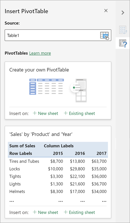
Select a table or range of data in your sheet and select Insert > PivotTable to open the Insert PivotTable pane.
-
You can either manually create your own PivotTable or choose a recommended PivotTable to be created for you. Do one of the following:
-
On the Create your own PivotTable card, select either New sheet or Existing sheet to choose the destination of the PivotTable.
-
On a recommended PivotTable, select either New sheet or Existing sheet to choose the destination of the PivotTable.
Note: Recommended PivotTables are only available to Microsoft 365 subscribers.
You can change the data sourcefor the PivotTable data as you are creating it.
-
In the Insert PivotTable pane, select the text box under Source. While changing the Source, cards in the pane won’t be available.
-
Make a selection of data on the grid or enter a range in the text box.
-
Press Enter on your keyboard or the button to confirm your selection. The pane will update with new recommended PivotTables based on the new source of data.

Get from Power BI
Use this option if your organization uses Power BI and you want to discover and connect to endorsed cloud datasets you have access to.
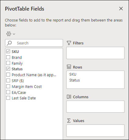
In the PivotTable Fields pane, select the check box for any field you want to add to your PivotTable.
By default, non-numeric fields are added to the Rows area, date and time fields are added to the Columns area, and numeric fields are added to the Values area.
You can also manually drag-and-drop any available item into any of the PivotTable fields, or if you no longer want an item in your PivotTable, drag it out from the list or uncheck it.
Summarize Values By
By default, PivotTable fields in the Values area will be displayed as a SUM. If Excel interprets your data as text, it will be displayed as a COUNT. This is why it’s so important to make sure you don’t mix data types for value fields.
Change the default calculation by right clicking on any value in the row and selecting the Summarize Values By option.
Show Values As
Instead of using a calculation to summarize the data, you can also display it as a percentage of a field. In the following example, we changed our household expense amounts to display as a % of Grand Total instead of the sum of the values.
Right click on any value in the column you’d like to show the value for. Select Show Values As in the menu. A list of available values will display.
Make your selection from the list.
To show as a % of Parent Total, hover over that item in the list and select the parent field you want to use as the basis of the calculation.
If you add new data to your PivotTable data source, any PivotTables built on that data source will need to be refreshed. Right-click anywhere in the PivotTable range, then select Refresh.
If you created a PivotTable and decide you no longer want it, select the entire PivotTable range and press Delete. It won’t have any effect on other data or PivotTables or charts around it. If your PivotTable is on a separate sheet which has no other data you want to keep, deleting the sheet is a fast way to remove the PivotTable.
-
Your data should be organized in a tabular format, and not have any blank rows or columns. Ideally, you can use an Excel table like in our example above.
-
Tables are a great PivotTable data source, because rows added to a table are automatically included in the PivotTable when you refresh the data, and any new columns will be included in the PivotTable Fields List. Otherwise, you need to either Change the source data for a PivotTable, or use a dynamic named range formula.
-
Data types in columns should be the same. For example, you shouldn’t mix dates and text in the same column.
-
PivotTables work on a snapshot of your data, called the cache, so your actual data doesn’t get altered in any way.
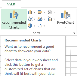
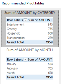
If you have limited experience with PivotTables, or are not sure how to get started, a Recommended PivotTable is a good choice. When you use this feature, Excel determines a meaningful layout by matching the data with the most suitable areas in the PivotTable. This helps give you a starting point for additional experimentation. After a recommended PivotTable is created, you can explore different orientations and rearrange fields to achieve your specific results. You can also download our interactive Make your first PivotTable tutorial.
-
Click a cell in the source data or table range.
-
Go to Insert > Recommended PivotTable.
-
Excel analyzes your data and presents you with several options, like in this example using the household expense data.
-
Select the PivotTable that looks best to you and press OK. Excel will create a PivotTable on a new sheet, and display the PivotTable Fields List

-
Click a cell in the source data or table range.
-
Go to Insert > PivotTable.
-
Excel will display the Create PivotTable dialog with your range or table name selected. In this case, we’re using a table called «tbl_HouseholdExpenses».
-
In the Choose where you want the PivotTable report to be placed section, select New Worksheet, or Existing Worksheet. For Existing Worksheet, select the cell where you want the PivotTable placed.
-
Click OK, and Excel will create a blank PivotTable, and display the PivotTable Fields list.
PivotTable Fields list
In the Field Name area at the top, select the check box for any field you want to add to your PivotTable. By default, non-numeric fields are added to the Row area, date and time fields are added to the Column area, and numeric fields are added to the Values area. You can also manually drag-and-drop any available item into any of the PivotTable fields, or if you no longer want an item in your PivotTable, simply drag it out of the Fields list or uncheck it. Being able to rearrange Field items is one of the PivotTable features that makes it so easy to quickly change its appearance.
PivotTable Fields list
-
Summarize by
By default, PivotTable fields that are placed in the Values area will be displayed as a SUM. If Excel interprets your data as text, it will be displayed as a COUNT. This is why it’s so important to make sure you don’t mix data types for value fields. You can change the default calculation by first clicking on the arrow to the right of the field name, then select the Field Settings option.
Next, change the calculation in the Summarize by section. Note that when you change the calculation method, Excel will automatically append it in the Custom Name section, like «Sum of FieldName», but you can change it. If you click the Number… button, you can change the number format for the entire field.
Tip: Since the changing the calculation in the Summarize by section will change the PivotTable field name, it’s best not to rename your PivotTable fields until you’re done setting up your PivotTable. One trick is to click Replace (on the Edit menu) >Find what > «Sum of«, then Replace with > leave blank to replace everything at once instead of manually retyping.
-
Show data as
Instead of using a calculation to summarize the data, you can also display it as a percentage of a field. In the following example, we changed our household expense amounts to display as a % of Grand Total instead of the sum of the values.
Once you’ve opened the Field Settings dialog, you can make your selections from the Show data as tab.
-
Display a value as both a calculation and percentage.
Simply drag the item into the Values section twice, right-click the value and select Field Settings, then set the Summarize by and Show data as options for each one.
If you add new data to your PivotTable data source, any PivotTables that were built on that data source need to be refreshed. To refresh just one PivotTable you can right-click anywhere in the PivotTable range, then select Refresh. If you have multiple PivotTables, first select any cell in any PivotTable, then on the Ribbon go to PivotTable Analyze > click the arrow under the Refresh button and select Refresh All.
If you created a PivotTable and decide you no longer want it, you can simply select the entire PivotTable range, then press Delete. It won’t have any affect on other data or PivotTables or charts around it. If your PivotTable is on a separate sheet that has no other data you want to keep, deleting that sheet is a fast way to remove the PivotTable.
Data format tips and tricks
-
Use clean, tabular data for best results.
-
Organize your data in columns, not rows.
-
Make sure all columns have headers, with a single row of unique, non-blank labels for each column. Avoid double rows of headers or merged cells.
-
Format your data as an Excel table (select anywhere in your data and then select Insert > Table from the ribbon).
-
If you have complicated or nested data, use Power Query to transform it (for example, to unpivot your data) so it is organized in columns with a single header row.
Need more help?
You can always ask an expert in the Excel Tech Community or get support in the Answers community.
PivotTable Recommendations are a part of the connected experience in Microsoft 365, and analyzes your data with artificial intelligence services. If you choose to opt out of the connected experience in Microsoft 365, your data will not be sent to the artificial intelligence service, and you will not be able to use PivotTable Recommendations. Read the Microsoft privacy statement for more details.
Related articles
Create a PivotChart
Use slicers to filter PivotTable data
Create a PivotTable timeline to filter dates
Create a PivotTable with the Data Model to analyze data in multiple tables
Create a PivotTable connected to Power BI Datasets
Use the Field List to arrange fields in a PivotTable
Change the source data for a PivotTable
Calculate values in a PivotTable
Delete a PivotTable
Data analysis in Excel is provided by construction of a table processor. A lot of the program’s resources are suitable for solving this task.
Excel positions itself as the best universal software product in the world for processing analytical information. From a small enterprise to large corporations, managers spend a significant part of their working hours analyzing their businesses activity. Let’s consider the main analytical tools in Excel and examples of their use in practice.
Excel analysis tools
One of the most attractive data analysis is «What-if Analysis». It is located in «DATA» tab.
Analysis tools of «What-if Analysis»:
- “Scenario Manager”. It is used to generate, change and save different sets of input data and the results of calculations for a group of formulas.
- «Goal Seek». It is used when the user knows the result of the formula, but the input information for this result is unknown.
- «Data Table». Used in situations when it is necessary to show the effect of variable values on formulas in the form of a table.
«Data Analysis». This is an Excel add-in. Helps find the best solution for a particular task.
Other tools for analysis:
Analyze data in Excel using built-in functions (mathematical, financial, logical, statistical, etc.).
Summary tables in data analysis
Excel uses summary tables to simplify the viewing, processing and consolidation of data.
The program will treat the entered information as a table, but not as a simple information set. But firstly you should format lists with values according to next steps:
- Go to the «INSERT» tab and click on the «Table» button CTRL+T.
- The «Create Table» dialog box appears.
- Specify the range of data (if it already exist) or the expected range (in which cells the table will be placed).
Set the check-mark in the box next to «Table with titles». Press Enter.
The specified default formatting style applies to the specified range.
You can compose the report using the «PivotTable».
- Activate any of the cells in the values range. We click the button «PivotTable» («INSERT» — «Tables» — «PivotTable»).
- In the dialog box you specify the range and place where to put the summary report (new sheet).
- The «PivotTable Fields» opens. The left side of the sheet is the report image; the right part is the tools for creating the summary report.
- Select the required fields from the list. Determine the values for the names of rows and columns. The report will be built on the left side of the sheet.
Creating a pivot table is already a way for analyzing information. Moreover, the user selects the information he needs at a particular moment for displaying. Then he can use other tools.
Analysis «What-if Analysis» in Excel: «Data Table»
This is a powerful tool for information analysis. Let’s consider the organization of information using the tool «What-if Analysis» — «Data Table».
Important conditions:
- data must be in one column or one line;
- the formula refers to one input cell.
The procedure for creating analysis:
- We enter the input values in a column. Enter the formula in the next column one line higher.
- We select a range of values including a column with input values and a formula A3:B12. Go to the «DATA» tab. Open the «What-if Analysis» tool. We click the «Data Table» button.
- There are two fields in the opened dialog box. Since we create a table with one input we enter the address only in the field «Column input cell:». If the input values are in lines (not in columns), we will enter the cell’s number in the field «Row input cell: » and click OK.
- Download enterprise analysis system
- Download analytical finance table
- Business profitability table
- Cash flow statement
- Example of a point method in financial and economic analytics
When using the features Excel, to analyze the enterprise activity, we use information from the balance sheet and income statement. Each user creates his own form, which reflects the features of the company and important information for decision-making.