
Excel for Microsoft 365 Excel for Microsoft 365 for Mac Excel 2021 Excel 2021 for Mac Excel 2019 Excel 2019 for Mac Excel 2016 Excel 2016 for Mac Excel 2013 Excel 2010 Excel 2007 Excel for Mac 2011 More…Less
By using What-If Analysis tools in Excel, you can use several different sets of values in one or more formulas to explore all the various results.
For example, you can do What-If Analysis to build two budgets that each assumes a certain level of revenue. Or, you can specify a result that you want a formula to produce, and then determine what sets of values will produce that result. Excel provides several different tools to help you perform the type of analysis that fits your needs.
Note that this is just an overview of those tools. There are links to help topics for each one specifically.
What-If Analysis is the process of changing the values in cells to see how those changes will affect the outcome of formulas on the worksheet.
Three kinds of What-If Analysis tools come with Excel: Scenarios, Goal Seek, and Data Tables. Scenarios and Data tables take sets of input values and determine possible results. A Data Table works with only one or two variables, but it can accept many different values for those variables. A Scenario can have multiple variables, but it can only accommodate up to 32 values. Goal Seek works differently from Scenarios and Data Tables in that it takes a result and determines possible input values that produce that result.
In addition to these three tools, you can install add-ins that help you perform What-If Analysis, such as the Solver add-in. The Solver add-in is similar to Goal Seek, but it can accommodate more variables. You can also create forecasts by using the fill handle and various commands that are built into Excel.
For more advanced models, you can use the Analysis ToolPak add-in.
A Scenario is a set of values that Excel saves and can substitute automatically in cells on a worksheet. You can create and save different groups of values on a worksheet and then switch to any of these new scenarios to view different results.
For example, suppose you have two budget scenarios: a worst case and a best case. You can use the Scenario Manager to create both scenarios on the same worksheet, and then switch between them. For each scenario, you specify the cells that change and the values to use for that scenario. When you switch between scenarios, the result cell changes to reflect the different changing cell values.
1. Changing cells
2. Result cell
1. Changing cells
2. Result cell
If several people have specific information in separate workbooks that you want to use in scenarios, you can collect those workbooks and merge their scenarios.
After you have created or gathered all the scenarios that you need, you can create a Scenario Summary Report that incorporates information from those scenarios. A scenario report displays all the scenario information in one table on a new worksheet.
Note: Scenario reports are not automatically recalculated. If you change the values of a scenario, those changes will not show up in an existing summary report. Instead, you must create a new summary report.
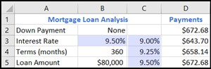
If you know the result that you want from a formula, but you’re not sure what input value the formula requires to get that result, you can use the Goal Seek feature. For example, suppose that you need to borrow some money. You know how much money you want, how long a period you want in which to pay off the loan, and how much you can afford to pay each month. You can use Goal Seek to determine what interest rate you must secure in order to meet your loan goal.

Cells B1, B2, and B3 are the values for the loan amount, term length, and interest rate.
Cell B4 displays the result of the formula =PMT(B3/12,B2,B1).
Note: Goal Seek works with only one variable input value. If you want to determine more than one input value, for example, the loan amount and the monthly payment amount for a loan, you should instead use the Solver add-in. For more information about the Solver add-in, see the section Prepare forecasts and advanced business models, and follow the links in the See Also section.
If you have a formula that uses one or two variables, or multiple formulas that all use one common variable, you can use a Data Table to see all the outcomes in one place. Using Data Tables makes it easy to examine a range of possibilities at a glance. Because you focus on only one or two variables, results are easy to read and share in tabular form. If automatic recalculation is enabled for the workbook, the data in Data Tables immediately recalculates; as a result, you always have fresh data.
Cell B3 contains the input value.
Cells C3, C4, and C5 are values Excel substitutes based on the value entered in B3.
A Data Table cannot accommodate more than two variables. If you want to analyze more than two variables, you can use Scenarios. Although it is limited to only one or two variables, a Data Table can use as many different variable values as you want. A Scenario can have a maximum of 32 different values, but you can create as many scenarios as you want.
If you want to prepare forecasts, you can use Excel to automatically generate future values that are based on existing data, or to automatically generate extrapolated values that are based on linear trend or growth trend calculations.
You can fill in a series of values that fit a simple linear trend or an exponential growth trend by using the fill handle or the Series command. To extend complex and nonlinear data, you can use worksheet functions or the regression analysis tool in the Analysis ToolPak Add-in.
Although Goal Seek can accommodate only one variable, you can project backward for more variables by using the Solver add-in. By using Solver, you can find an optimal value for a formula in one cell—called the target cell—on a worksheet.
Solver works with a group of cells that are related to the formula in the target cell. Solver adjusts the values in the changing cells that you specify—called the adjustable cells—to produce the result that you specify from the target cell formula. You can apply constraints to restrict the values that Solver can use in the model, and the constraints can refer to other cells that affect the target cell formula.
Need more help?
You can always ask an expert in the Excel Tech Community or get support in the Answers community.
See Also
Scenarios
Goal Seek
Data Tables
Using Solver for capital budgeting
Using Solver to determine the optimal product mix
Define and solve a problem by using Solver
Analysis ToolPak Add-in
Overview of formulas in Excel
How to avoid broken formulas
Detect errors in formulas
Keyboard shortcuts in Excel
Excel functions (alphabetical)
Excel functions (by category)
Need more help?
Want more options?
Explore subscription benefits, browse training courses, learn how to secure your device, and more.
Communities help you ask and answer questions, give feedback, and hear from experts with rich knowledge.
Create Different Scenarios | Scenario Summary | Goal Seek
What-If Analysis in Excel allows you to try out different values (scenarios) for formulas. The following example helps you master what-if analysis quickly and easily.
Assume you own a book store and have 100 books in storage. You sell a certain % for the highest price of $50 and a certain % for the lower price of $20.

If you sell 60% for the highest price, cell D10 calculates a total profit of 60 * $50 + 40 * $20 = $3800.
Create Different Scenarios
But what if you sell 70% for the highest price? And what if you sell 80% for the highest price? Or 90%, or even 100%? Each different percentage is a different scenario. You can use the Scenario Manager to create these scenarios.
Note: You can simply type in a different percentage into cell C4 to see the corresponding result of a scenario in cell D10. However, what-if analysis enables you to easily compare the results of different scenarios. Read on.
1. On the Data tab, in the Forecast group, click What-If Analysis.

2. Click Scenario Manager.

The Scenario Manager dialog box appears.
3. Add a scenario by clicking on Add.

4. Type a name (60% highest), select cell C4 (% sold for the highest price) for the Changing cells and click on OK.

5. Enter the corresponding value 0.6 and click on OK again.

6. Next, add 4 other scenarios (70%, 80%, 90% and 100%).
Finally, your Scenario Manager should be consistent with the picture below:

Note: to see the result of a scenario, select the scenario and click on the Show button. Excel will change the value of cell C4 accordingly for you to see the corresponding result on the sheet.
Scenario Summary
To easily compare the results of these scenarios, execute the following steps.
1. Click the Summary button in the Scenario Manager.
2. Next, select cell D10 (total profit) for the result cell and click on OK.

Result:

Conclusion: if you sell 70% for the highest price, you obtain a total profit of $4100, if you sell 80% for the highest price, you obtain a total profit of $4400, etc. That’s how easy what-if analysis in Excel can be.
Goal Seek
What if you want to know how many books you need to sell for the highest price, to obtain a total profit of exactly $4700? You can use Excel’s Goal Seek feature to find the answer.
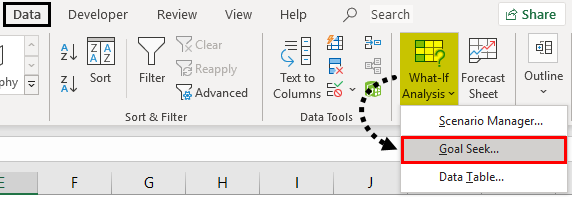
1. On the Data tab, in the Forecast group, click What-If Analysis.
2. Click Goal Seek.

The Goal Seek dialog box appears.
3. Select cell D10.
4. Click in the ‘To value’ box and type 4700.
5. Click in the ‘By changing cell’ box and select cell C4.
6. Click OK.

Result. You need to sell 90% of the books for the highest price to obtain a total profit of exactly $4700.

Note: visit our page about Goal Seek for more examples and tips.
What-If Analysis in Excel is a tool that helps us create different models, scenarios, and Data Tables. This article will look at the ways of using What-If Analysis.
Table of contents
- What is a What-If Analysis in Excel?
- #1 Scenario Manager in What-If Analysis
- #2 Goal Seek in What-If Analysis
- #3 Data Table in What-If Analysis
- Things to Remember
- Recommended Articles
We have three parts of What-If Analysis in Excel. They are as follows:
- Scenario Manager
- Goal Seek in Excel
- Data Table in Excel
You can download this What-If Analysis Excel Template here – What-If Analysis Excel Template
#1 Scenario Manager in What-If Analysis
As a business head, it is important to know the different scenarios of your future project. Based on the scenarios, the business head will make decisions. For example, you are going to undertake one of the important projects. You have done your homework and listed all the possible expenditures from your end, and below is the list of all your expenses.
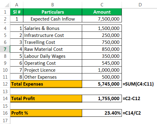
The expected cash flow from this project is $75 million, which is in cell C2. Total expenses comprise all your fixed and variable expenses, the total cost is $57.45 million in cell C12. Total profit is $17.55 million in cell C14, and profit % is 23.40% of your cash inflow.
It is the basic scenario of your project. Now, you need to know the profit scenario if some of your expenses increase or decrease.
Scenario 1
- In a general case scenario, you have estimated the “Project License” cost to be $10 million, but you are sure anticipating it to be $15 million
- Raw material costs to be increased by $2.5 million
- Other expensesOther expenses comprise all the non-operating costs incurred for the supporting business operations. Such payments like rent, insurance and taxes have no direct connection with the mainstream business activities.read more to be decreased by 50 thousand.
Scenario 2
- The “Project Cost” to be at $20 million
- The “Labor Daily Wages” to be at $5 million
- The “Operating Cost” is to be at $3.5 million
Now, you have listed out all the scenarios in the form. Based on these scenarios, you need to create a table about how it will impact your profit and profit %.
To create What-If Analysis scenarios, follow the below steps.
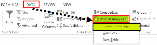
- Go to DATA > What-If Analysis > Scenario Manager.

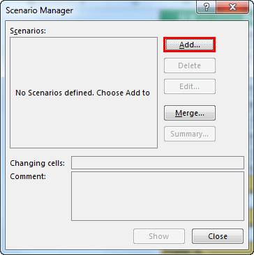
- Once you click “Scenario Manager,” it will show you below the dialog box.

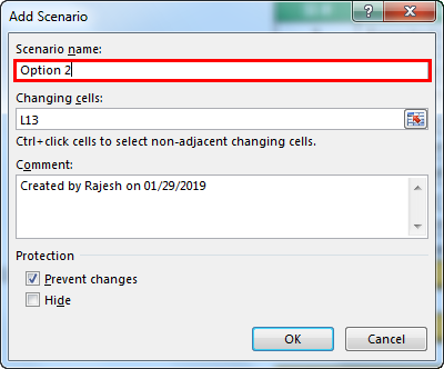
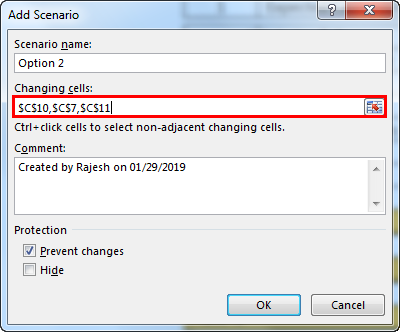
- Click on “Add.” Then, give “Scenario name.”

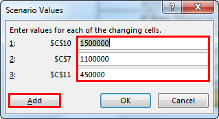
- In changing cells, select the first scenario changes you have listed out. The changes are Project License (cell C10) at $15 million, Raw Material Cost (cell C7) at $11 million, and Other Expenses (cell C11) at $4.5 million. Mention these three cells here.
- Click on “OK.” It will ask you to mention the new values as listed in scenario 1.

- Do not click on “OK” but click on “OK Add.” It will save this scenario for you.
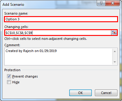
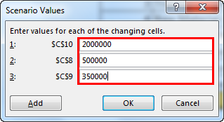
- Now, it will ask you to create one more scenario. As we listed in scenario 2, make the changes. This time we need to change Project Cost (C10), Labour Cost (C8), and Operating Cost (C9).
- Now, add new values here.
- Now click on “OK.” It will show all the scenarios we have created.
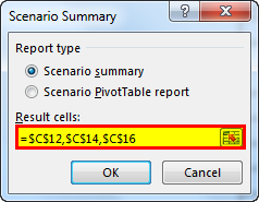
- Click on “Scenario summary.” It will ask you which result cells you want to change. Here, we need to change the Total Expense Cell (C12), Total Profit Cell (C14), and Profit % cell (C16).

- Click on “OK.” It will create a summary report for you in the new worksheet.


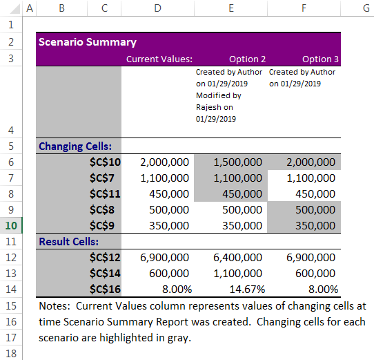
Total Excel has created three scenarios even though we have supplied only two scenario changes because Excel will show existing reports as one scenario.
From this table, we can easily see the impact of changes in pour profit %.
#2 Goal Seek in What-If Analysis
Now, we know the Scenario Manager’s advantage. What-if-Analysis Goal Seek can tell you what you must do to achieve the target.
Andrew is a class 10th student. His target is to achieve an average score of 85 in the final exam. He has already completed 5 exams and left with only 1 exam. Therefore, in the completed 5 exams.
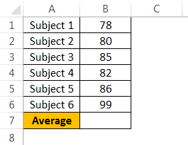
To calculate the current average, apply the average formula in the B7 cell.
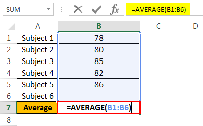
The current average is 82.2.
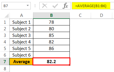
Andrew’s GOAL is 85. His current average is 82.2. He is short by 3.8 with one exam.
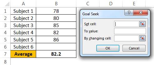
Now, the question is how much he has to score in the final exam to eventually get an overall average of 85. It can be found by the What-If Analysis GOAL SEEK tool.
- Step 1: Go to DATA > What-If Analysis > Goal Seek.

- Step 2: It will show you below the dialog box.
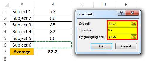
- Step 3: Here, we need to set the cell first. “Set cell” is nothing but which cell we need for the final result, i.e., our overall average cell (B7). Next is “To value.” Again, Andrew’s overall average GOAL is nothing but for what value we need to set the cell (85).
The next and final step is changing which cell you want to see the impact on. So, we need to change cell B6, the cell for the final subject’s score.
- Step 4: Click on “OK.” Excel will take a few seconds to complete the process, but it eventually shows the result like the one below.
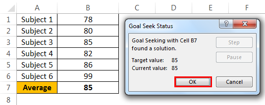
Now, we have our results here. To get an overall average of 85, Andrew has to score 99 in the final exam.
#3 Data Table in What-If Analysis
We have already seen two wonderful techniques under What-If Analysis in Excel. First, the Data Table can create different scenario tables based on the variable change. We have two kinds of Data Tables here: one variable Data Table and a “Two-variable data tableA two-variable data table helps analyze how two different variables impact the overall data table. In simple terms, it helps determine what effect does changing the two variables have on the result.read more.” This article will show you One variable data table in ExcelOne variable data table in excel means changing one variable with multiple options and getting the results for multiple scenarios. The data inputs in one variable data table are either in a single column or across a row.read more.
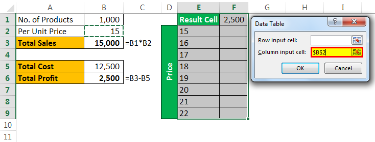
Assume you are selling 1,000 products at ₹15, your total anticipated expense is ₹12,500, and your profit is ₹2,500.
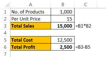
You are not happy with the profit you are getting. Your anticipated profit is ₹7,500. You have decided to increase your per-unit price to increase your profit, but you do not know how much you need to increase.
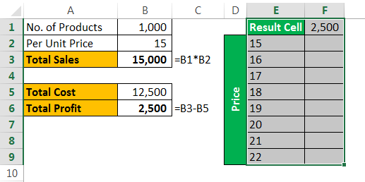
Data tables can help you. Create a table below.

Now, in the cell, F1 links to the “Total Profit” cell, B6.

- Step 1: Select the newly created table.
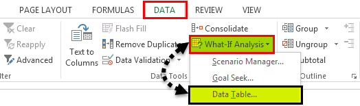
- Step 2: Go to DATA > What-if Analysis > Data Table.
- Step 3: Now, you will see below dialog box.
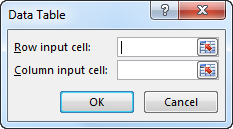
- Step 4: Since we are showing the result vertically, leave the ”Row input cell.” In the “Column input cell,” select cell B2, which is the original selling price.
- Step 5: Click on “OK” to get the results. It will list out profit numbers in the new table.
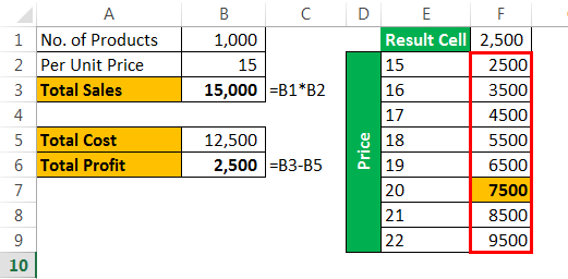
So, we have our Data Table ready. To profit from ₹7,500, you need to sell at ₹20 per unit.
Things to Remember
- The What-If Analysis data table can be performed with two variable changes. Refer to our article on What-If Analysis two-variable Data Table.
- What-If Analysis Goal Seek takes a few seconds to perform calculations.
- What-If Analysis Scenario Manager can give a summary with input numbers and current values together.
Recommended Articles
This article is a guide to What-If Analysis in Excel. Here, we discuss three types of What-If Analysis in Excel such as 1) Scenario Manager, 2) Goal Seek, 3) Data Tables along with practical examples, and a downloadable Excel template. You may learn more about Excel from the following articles: –
- Pareto Analysis in ExcelA pareto chart is a graph which is a combination of a bar graph and a line graph, indicates the defect frequency and its cumulative impact. It helps in finding the defects to observe the best possible and overall improvement measure.read more
- Goal Seek in VBA
- Sensitivity Analysis in Excel
Анализ «Что Если» в Excel позволяет попробовать различные значения (сценарии) для формул.
Следующий пример поможет Вам освоить Анализ «что если» быстро и легко.
Предположим, у вас есть книжный магазин и есть 100 книг на продажу. Вы продаете определенный % книг по самой высокой цене в $ 50 и определенный % книг по более низкой цене $ 20.

Если вы продаете 60% книг по самой высокой цене, ячейка D10 вычисляет общую прибыль в размере 60 * $ 50 + 40 * $ 20 = $ 3800.
Скачать рассматриваемый пример Вы можете по этой ссылке: Пример анализа «что если» в Excel.
Создание различных сценариев
Что будет, если Вы продадите 70% книг по высокой цене? А что будет, если Вы продадите 80% книг? Или 90%, или 100%? Каждый другой процент продажи книг — это различный сценарий.
Вы можете использовать «Диспетчер сценариев» для создания этих сценариев.
Примечание: Вы можете просто ввести другой процент в ячейку C4, что бы увидеть результат в ячейке C10. Однако, Анализ «что если» позволит Вам сравнить результаты различных сценариев.
Итак, приступим.
1. На вкладке Данные выберите Анализ «что если» и выберите Диспетчер сценариев из списка.
Откроется диалоговое окно Диспетчер сценариев.

2. Добавьте сценарий, нажав на кнопку Добавить.

3. Введите имя (60% книг по высокой цене), выберите ячейку C4 (% книг, которые продаются по высокой цене) для изменяемой ячейки и нажмите на кнопку OK.

4. Введите соответствующее значение 0,6 и нажмите на кнопку OK еще раз.

5. Далее, добавьте еще 4 других сценария (70%, 80%, 90% и 100% соответсвенно).
И, наконец, ваш Диспетчер сценариев должен соответствовать картинке ниже:

Примечание: чтобы увидеть результат сценария, выберите сценарий и нажмите на кнопку Вывести. Excel изменит значение ячейки C4 в соответствии со сценарием, что бы Вы смогли увидеть результат на листе.
Отчет по сценариям
Для того, чтобы легко сравнить результаты этих сценариев, выполните следующие действия:
1. Кликните по кнопке «Отчет» в Диспетчере сценариев.
2. Далее, выберите ячейку C10 (итого выручка) в качестве ячейки результата и нажмите ОК.

Результат:

Вывод: Если вы продаете 70% книг по высокой цене, то Вы получите общую выручку в размере $ 4100, если Вы продаете 80% книг по высокой цене, то Вы получаете общую прибыль в размере $ 4400 и т.д. Вот как легко можно использовать Анализ «что если» в Excel.
Подписывайтесь на нас в социальных сетях, оставляйте комментарии к статье. Надеюсь пример использования анализа «что если» в Excel Вам понравился.
What If Analysis In Excel (Table of Contents)
- Overview of What-if Analysis in Excel
- Examples of What-if Analysis in Excel
Overview of What If Analysis in Excel
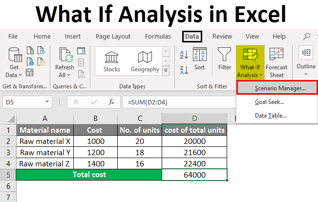
What-if analysis in Excel is used to test more than one value for a different formula on the basis of multiple scenarios. For this, we must have data of such kind where, for a single parameter, we would have 2 or more values for comparison. Go to the Data menu tab and click on the What-If Analysis option under the Forecast section. Select the scenario manager and give a scenario name and select the cell which contains the scenario value. By this, we can enter multiple scenarios. Now from the Goal Seek option from What-If Analysis, select the value we want to compare.
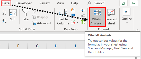
What if the analysis is available in the “forecast” section under the “Data” tab.
There are three different kinds of tolls in the What-if analysis. Those are:
1. Scenario manager
2. Goal Seek
3. Data table
We will see each one with related examples.
Examples of What If Analysis in Excel
Here are some examples given below:
You can download this What if Analysis Excel Template here – What if Analysis Excel Template
Example #1 – Scenario Manager
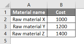
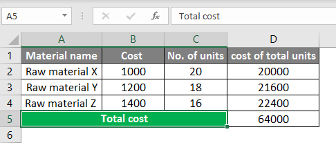
The scenario manager helps to find the results for different scenarios. Let’s consider a company that wants to buy raw materials for their organization’s needs. Due to the scarcity of funds, the company wants to understand how much cost will happen for different possibilities of buying.
In these cases, we can use the scenario manager for applying different scenarios to understand the results and make the decision accordingly. Now consider Raw material X, Raw material Y, and Raw material Z. We know the price of each, and we want to know how much amount need for different scenarios.
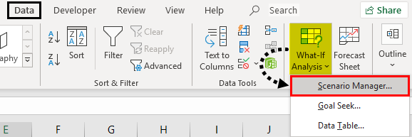
Now we need to design 3 scenarios like High volume purchase, Medium volume purchase, and Low volume purchase. For that, click on What if analysis and select Scenario manager.
Once we select the scenario manager, the following window will open.
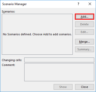
As shown in the screenshot, currently, there were no scenarios; if we want to add scenarios, we need to click on the “Add” option available.
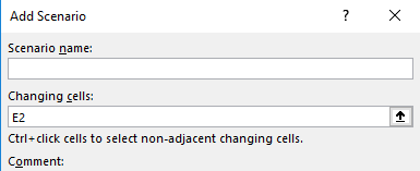
Then it will ask for the Scenario name and changing cells. Give scenario name whatever you want as per your requirement. Here I am giving “High volume.”
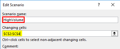
Changing cells is the range of cells that your scenario values for different scenarios. Suppose if we observe the below screenshot. No. of units will change in each scenario; that is the reason for changing cells; we used C2:C4, which means C2, C3, and C4.
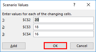
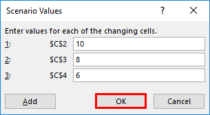
Once you give the change values, click on “OK”, then it will ask for the changing values for the High volume scenario. Input the values for high volume scenario and then click on “Add” to add another scenario “, Medium Volume.”
Give name as “Medium volume” and give the same range and click Ok then it will ask for values.
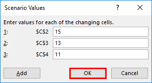
Again, click on “Add” and create one more scenario “, Low volume”, with low values like below.
Once all scenarios have done, click on “Ok” You will find the below screen.
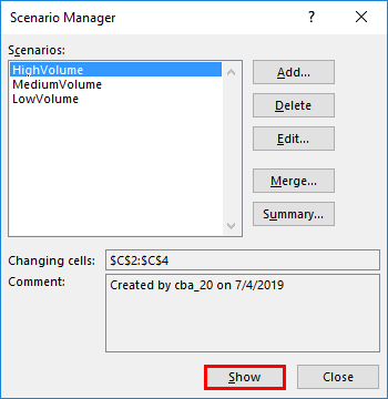
We can find all the scenarios on the “Scenarios” screen. Now we can click on each scenario and click on Show; then you will find the results in excel; otherwise, we can view all the scenarios by clicking on the option “Summary.”
If we click on the scenario wise, the results will be changing in excel as below.
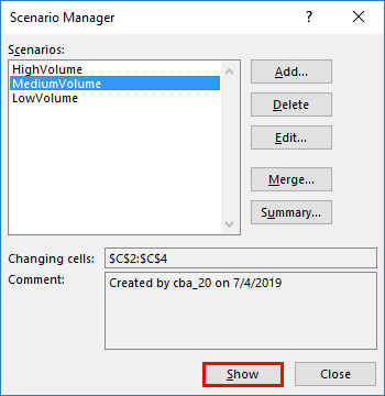
Whenever you click on the scenario and show the results at the back will change. If we want to see all the scenarios at a time to compare with others, click on the summary the following screen will come.
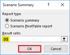
Select ‘Scenario Summary” and give the “Results Cells” here; the total results will be in D5; hence I given D5, click on ‘Ok’. Then a new tab will be created with the name “Scenario summary.”
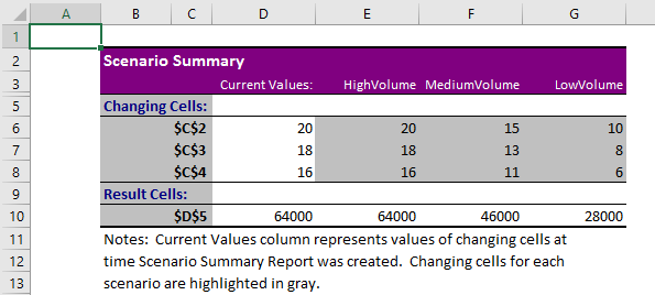
Here the columns in grey color are the changing values, and the column in white color is the current value which was the last selected scenario results.
Example #2 – Goal Seek
Goal seek helps to find the input for the known output or required output.
Suppose we will take a small example of product sale. Suppose we know that we want to sell the product at an additional price of 200 than product cost then we want to know what is the percentage we are earning the profit.
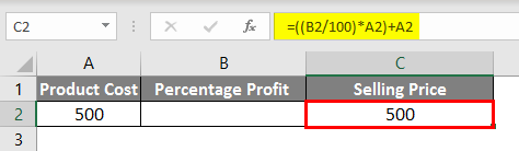
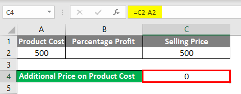
Observe the above screenshot product cost is 500, and I have given the formula for finding the percentage profit, which you can observe in the formula bar. In one more cell, I gave the formula for the additional price which we want to sell.
Now use Goal Seek to find the profit percentage of the different additional prices on the product’s product cost and selling price.
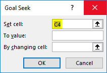
When we click on the “Goal seek”, the above pop up will come. In the set, the cell gives the cell position where we are going to give the output value here the additional price amount we know which we are giving in cell C4.
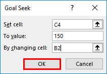
The “To Value” is the value at what additional price we want to cell 150 rupees additional to the product cost, and the changing cell is B2 where percentage changes. Click on “Ok” and see how much percentage profit if we sell an additional 150 rupees.
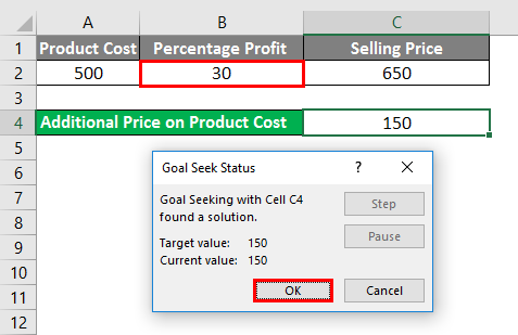
The profit percentage is 30, and the selling price should be 650. Similarly, we can check for different targeted values. This goal seeks to help to find the EMI calculations etc.
Example #3 – Data Tables in What If Analysis
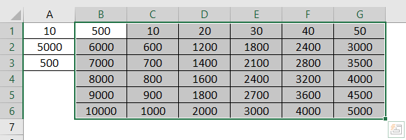
Now we will see the Data table. We will consider a very small example to understand better. Suppose we want to know the 10%, 20%, 30%, 40% and 50% of 5000 similarly, we want to find the percentages for 6000, 7000, 8000, 9000 and 10000.
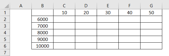
We have to get the percentages in each combination. In these situations, the Data table will help to find the output for a different combination of inputs. Here in Cell B3 should get 10% of 6000 and B4 10% of 7000 and so on. Now we will see how to achieve this. First, create a formula to perform this.
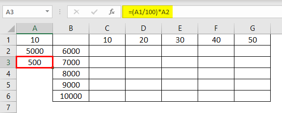
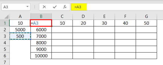
If we observe the above screenshot, the part marked with a box is the example. In A3, we have the formula to find the percentage from A1 and A2. So inputs are A1 and A2. Now take the result of A3 to A1 as shown in the below screenshot.
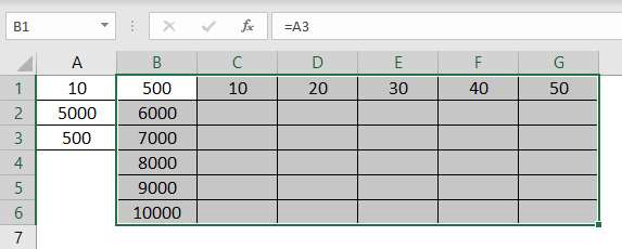
Now select the entire table to apply the Data table of What if Analysis as shown in the below screenshot.
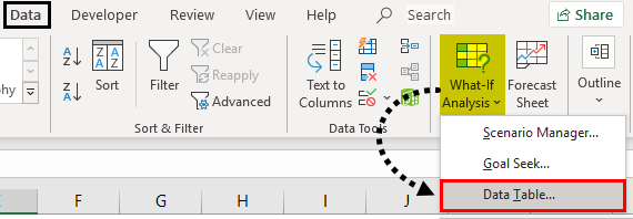
Once selected, click on the “Data” then “What If Analysis” from that dropdown select data table.
Once you select “Data table”, the below pop-up will come.
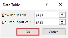
In “Row Input cell”, give the cell address where the row inputs should input, which means here row inputs are 10, 20, 30,40, and 50. Similarly, give “Column input cell” as A2 here column inputs are 6000, 7000, 8000, 9000, and 10,000. Click on “Ok”, then results will appear in the form of a table as shown below.
Things to Remember
- What if Analysis is available under the “Data” menu on the top.
- It will have 3 features 1. Scenario manager 2. Goal seeks and 3. Data table.
- Scenario manager helps to analyze different situations.
- Goal seek helps to know the right input value for the required output.
- Data table helps to get results of different inputs in row-wise and column-wise.
Recommended Articles
This is a guide on What if Analysis in Excel. Here we discuss three different tools in What if Analysis and the examples and downloadable excel template. You may also look at the following articles to learn more –
- Pareto Analysis in Excel
- Excel Quick Analysis
- Excel Regression Analysis
- Excel Tool for Data Analysis