
Contents
- Tools, Calculators and Simulations
- Dashboards and Reports with Charts
- Automate Jobs with VBA macros
- Solver Add-in & Statistical Analysis
- Data Entry and Lists
- Games in Excel!
- Educational use with Interactive features
- Create Cheatsheets with Excel
- Diagrams, Mockups, Gantt Charts
- Fetch live data from web
- Excel as a Database
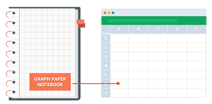
Excel is one of the most used software in today’s digital world. Most people quickly open up an Excel file when they need to write or calculate anything. It is like “paper”. (remember those graph notebooks from school times..)
Actually, this is not only specific to Microsoft’s Excel but most of the spreadsheet software like open office or google sheets. However, we will focus on Excel and what can you do with it today, as it offers huge flexibility you will discover below.
Let’s start with the main usage areas of Excel. As we all know, spreadsheets are designed to make calculations easier. So they contain “formulas”. They allow us to make basic math like summing, multiplying, finding average as well as advanced calculations like regression analysis, conversions, and so on.
When we combine these powerful math features with some tables, lists, or other UI elements, we can come up with a calculator. And most of the time they will be dynamic (meaning that when you change a parameter all the rest of the calculations will adapt accordingly)
Below see an example from our past studies as Someka:
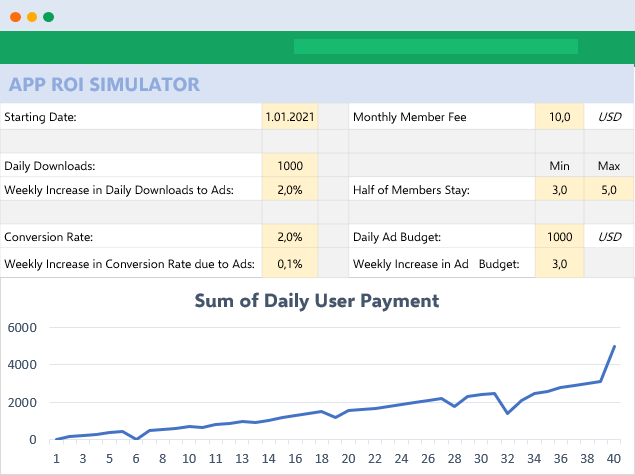
We have built this calculator for an app development company executive. He was changing the parameters he wants and sees the outcomes immediately.
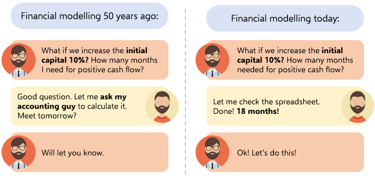
This is great especially when you try to make big “models” in excel. Financial Modeling is one of the most used application areas of these big models. If we tried to do this with pen-paper (which used to be the way once upon a time) it would be horrible I guess:
Financial modeling is also being used to test the excel skills of experts. They even make a competition for it: ModelOff
We also have a tool for startups to make a feasibility study playing with their own variables:
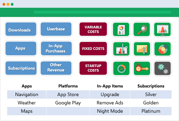
This is a comprehensive Feasibility Study Excel Template for app startups with download projections, costs, financial calculations, charts, dashboard, and more.
The business world is demanding. It is not enough just to make the calculations, set up your tables, and write the text. You have to create pie charts, trends, line graphs, and many more. Whether you are getting prepared for your pitch or make a presentation in your company, you can use Excel’s chart features.
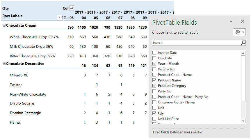
Pivot Tables
One of the greatest features which Excel offers is Pivot tables. This is an advanced Excel tool that helps you create dynamic summary reports from raw data very easily. After you create your table you can play with parameters easily with a drag and drop interface.
It looks like this:
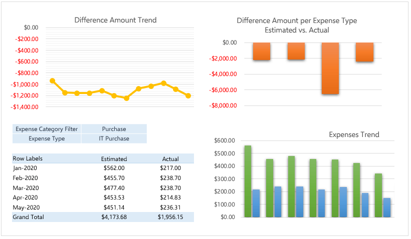
Dashboards
Complex excel models do have lots of variables, calculations, and settings. And instead of managing all variables one by one on different sheets, different places it is a very good idea to put them together like a “control panel”.
You can think dashboards as cockpits of planes.
Recently dashboards became very popular. There are lots of training videos about how to build and design control panels for our excel models. Actually, they are not so different from the rest of the calculations.
But the main idea is: if there is something you may want to change, later on, don’t write it directly in the formula but bind it to a variable.
Let’s say you are building a sales report for your manager. He asks you to make the file changeable so that he can see the results in US dollars or Euros according to the situation. Instead of writing an Fx rate into the calculations, you should bind this to a cell that you can play with later on.
Like this:
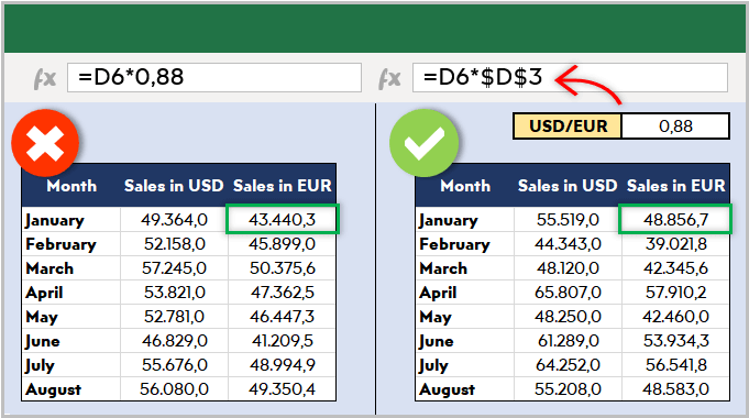
This may seem so obvious to some of you. But this is the basic approach of all dashboards in excel files. Of course, you can improve it with more complex formulas, buttons, cool charts, and even VBA but the main idea stands still.
Here is an example of a complete set of the dashboard:
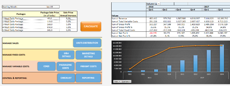
Or a dashboard for a livestock feasibility study:
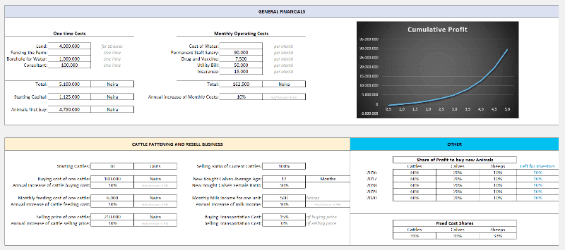
If you are interested in Sales Dashboards, you may want to check out our Excel template:
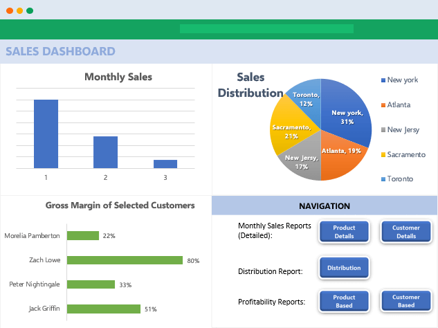
This is an interactive Sales Report Template in Excel. Features a dashboard with profitability, sales analysis and charts.
Other than that, Marketing ROI Calculator would be very helpful to prioritize your marketing campaigns in Excel:
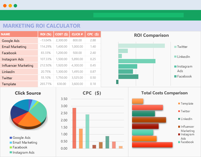
It will provide essential metrics and help you to manage all your marketing campaign channels in one place.
Most of the users who use Excel extensively are already coding. But if you ask them whether they know how to code most probably they will say no. Of course, writing formulas is a very small part of the things you can do with VBA. It is a strong programming language that lets you create small scripts (macros), user forms, user-defined functions, add-ins, and even games! (which we will touch below separately)
I will not dive into VBA here since it is a detailed area. But there are some basic things that will be beneficial to know for those who use Excel often:
- You can record macros for repeating jobs: You don’t need to code from scratch. Just click on the record macro button and it will write the code for you in the background. (If you want, you can modify later on)
- It extends the borders of Excel world. If you feel like you are limited somehow in Excel, you are more like an advanced user. It is time to get a little bit into VBA.
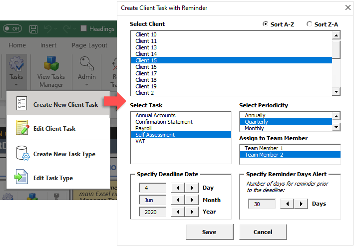
- You can create user forms with VBA only. If you see something like this, know that it is using VBA:
VBA is quite powerful and if you work with Excel extensively you won’t regret learning a bit. For example wouldn’t it be nice if you could send bulk emails from an Excel spreadsheat with a button click?
It is not surprising for spreadsheet software like Excel to offer advanced math techniques to make more complicated studies. (To be honest, I am not a statistics expert but with an engineering background, I will try to do my best to explain the basics. Feel free to correct me if I’m wrong)
Data analysis is a trending concept for recent years with the development of powerful computers and improved software. We are collecting and recording much much more data compared to the past. Take a look at this chart to understand what I mean:

Especially this part:
“more data has been created in the past two years than in the entire previous history of the human race”
It is a bit frightening, isn’t it? Ok, we are not going to dive into the “Big Data” world. Let’s get back to our humble excel world.
As we collect this much data, some people will want to analyze it. Otherwise, it makes no sense to spend billions of dollars on those data centers. Excel has built-in functions for basic descriptive statistics methods like Mean, Median, Mode, Standard Deviation, Variance etc.
But if we want to go a bit further I will mention two Excel features (actually add-ins) at this step: Solver and Regression Analysis
Solver
Have you ever heard of “optimization”? When we have more than one parameters that affect the outcome, we can only have a most optimized solution rather than a maximum solution. This may sound weird but it is very valid in our daily lives.
One of the simplest and popular examples is: Farmer Fence Optimization Problem
“A farmer owns 500 meters of the fence and wants to enclose the largest possible rectangular area. How should he use his fence?”
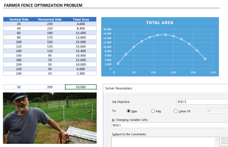
This is a very simple example to explain what a solver does. But actually, you can run much more complicated data sets with Solver.
Regression Analysis
Since this is a bit advanced topic for this blog post, I will only touch the surface.
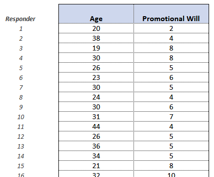
In most simple terms, regression analysis helps you find the correlation between the variables. For example, you may want to know what is the relation between the number of birds flown over your head and the money you earned today. (sorry for the silly example. No, I am not curious about it  You will need to gather sample data and put in an analysis to see if there is any correlation.
It seems something like this:
You put your data:
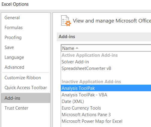
Run the regression from Analysis Toolpak:
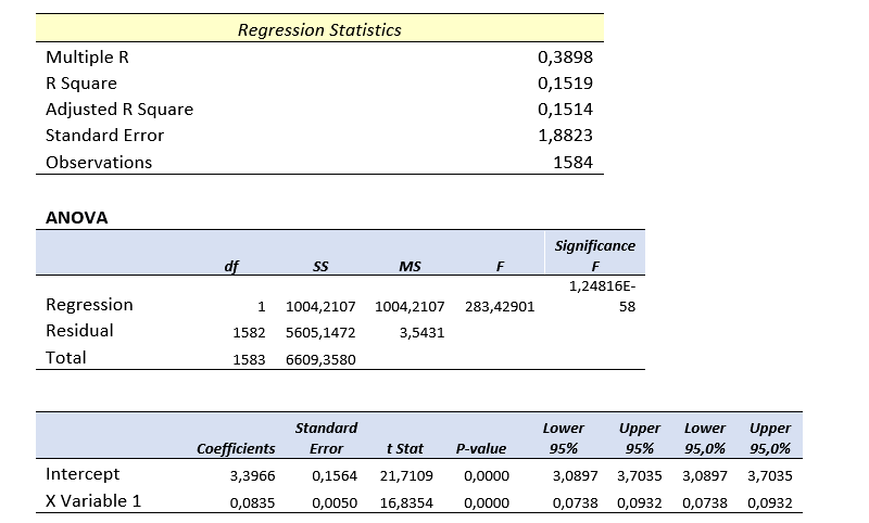
And get results something like this:
Of course, there is much more sophisticated software to run data analysis. However, there is a joke in business intelligence communities:
- What is the most used feature of any business intelligence solution?
- It is “Export to Excel”
Looks like we won’t stop using Excel anytime soon.
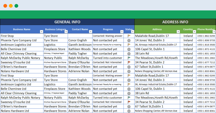
Coming back from boring data analysis world, let’s mention the simplest and most handy usage area of excel: Make Lists!
It is already self-explaining so I won’t bother with the details. When you want to list down some simple data, take notes, create to-do lists, or anything. Just open the excel and write it down. Did we mention that “paper alternative” thing? Oh yes, we did.
A lead list example:
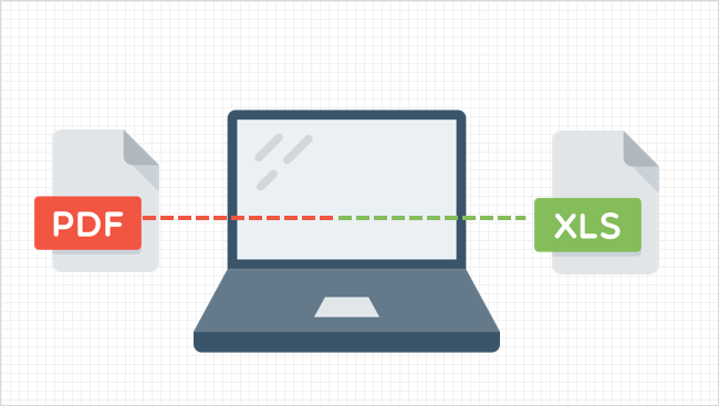
You can also convert PDF files into Excel files in order to make it easier to work on. This can be done automatically with some software. But some pdf files cannot be processed automatically (like handwritten documents, scanned invoices, etc). You will need to do it manually.
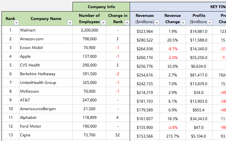
When you want to play with the data on a web page, you can easily copy-paste it into an excel file and then you can sort, filter or do anything you want:
For example, Fortune 500 US List:
Everybody loves to-do lists. And we have created useful to-do list in Excel for business or personal uses. Check it out, it is free:
To-Do List Excel Template
We already mentioned this in the VBA section above. But it is worth to talk a bit more.
Visual Basic allows you to code complex things like games as well. But of course, don’t expect a GTA or FIFA. Things like chess, sudoku, or Monopoly is OK. But, a few people have gone far and created more complicated things, like an RPG game. Take a look at this:
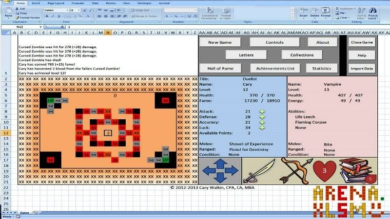
This game has been created by an accountant, Cary Walkin. I know it doesn’t look great but it is in Excel! (you can play it at the office  )
)
Another example:

A flight simulator in Excel?? Is it the same thing we use to sum up the sales figures? Lol yeah.
You can also embed flash games into Excel (like Super Mario, Angry Birds or whatever) But I count them off as they are not built with VBA.
As we mentioned in the Financial Modeling section, Excel is quite good for creating dynamic results according to the inputs. We get the benefit of this to create interactive tools.
One example that comes to my mind is this spreadsheet, guys from San Francisco have prepared:
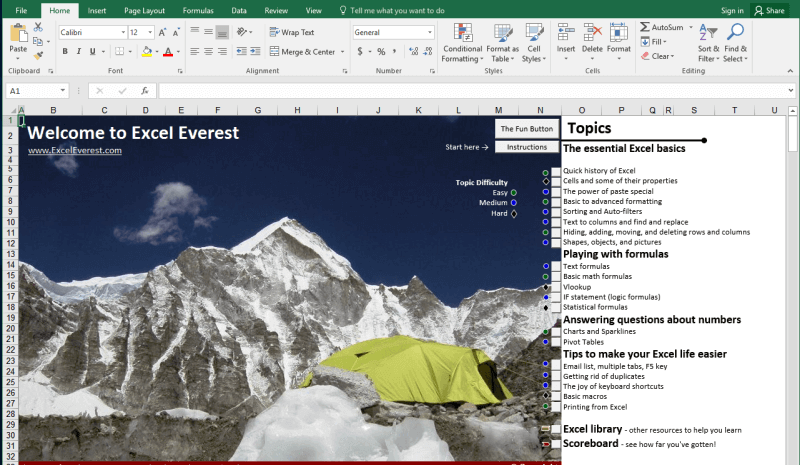
I haven’t tried it myself but an Excel tutorial in Excel. Liked the idea!
Another similar interactive Excel learning tool is from Keyskillset:
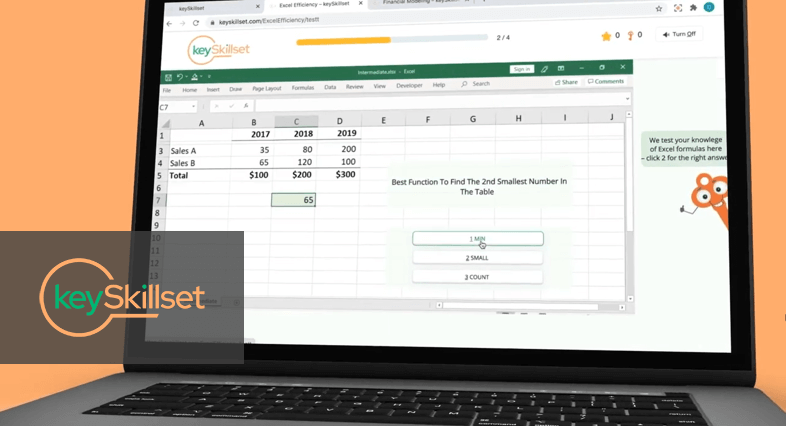
Actually, this is not completely in Excel and works as separate software but I liked how they combine the Excel training with gamification features.
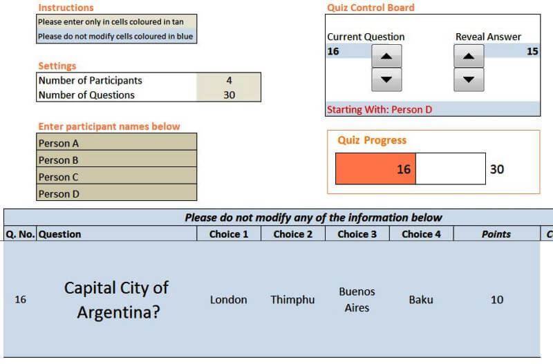
Quizzes are good tools for interactive learning and you can prepare in Excel as well. A quizmaster template from indzara.com:
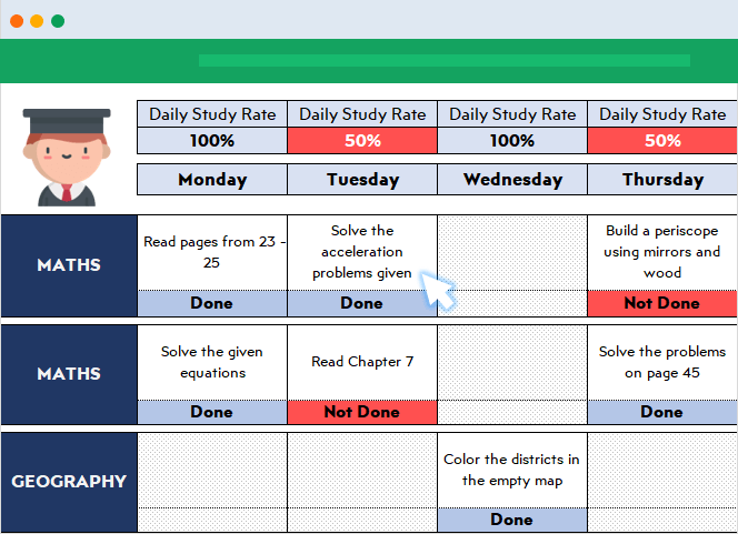
A student lesson plan template in excel which we have prepared recently:
You can learn Excel in Excel!
As said: Practice Makes Perfect!
You can test your Excel skills in Excel with Excel Formulas Trainer:
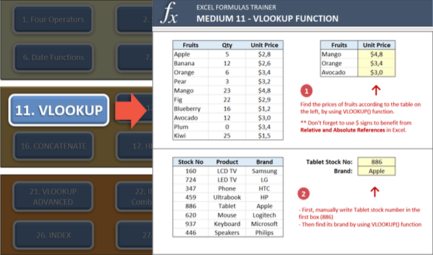
This is actually an Excel template prepared with VBA macros and basically works as a practice worksheet. It has 30 sections and around 100 questions. You can learn VLOOKUP, IF and much more excel formulas by doing. If you like the idea of “learning by doing”, then it is worth to check.
Also, this online course from GoSkills is for everyone as well, covering beginner, intermediate and advanced lessons.
By cheat sheets, we don’t refer to the piece of paper with information written down on it that an unethical person might create if they weren’t prepared for a test. What we mean is a reference tool that provides simple, brief instructions for accomplishing a specific task. We use this term because it is highly popular recently.
For example, this is a cheat sheet:
This compacted and summarized info is very useful in many aspects. When you try to memorize things, lookup, reference, etc. And can be easily created with Excel. Let’s make a Google search for a cheat sheet made in Excel.
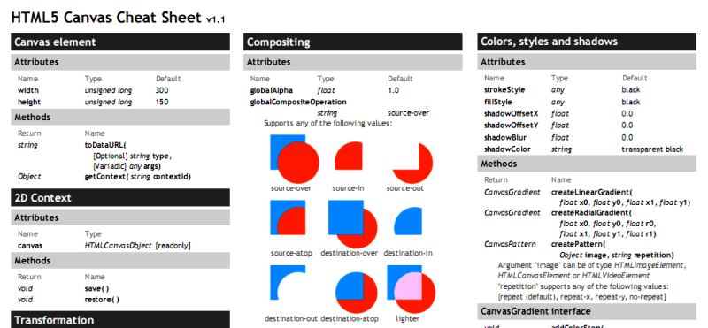
This one is from Dave Child (cheatography.com) and I was also using this one I first learned HTML:
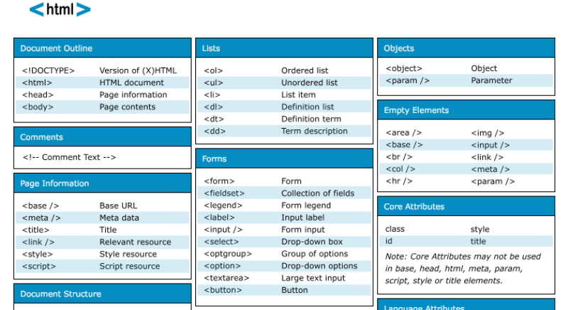
The last example is an Excel Cheatsheet made for Excel shortcuts:
Of course, if you are looking for stylish infographics and cheat sheets, you should check out design software.
I know Excel is maybe not the best tool to do these. There are great programs or websites to make mockups, diagrams, brainstorming, mind-mapping, or project scheduling. But there are habits as well. Even though I am very open to try and use these kinds of brand-new tools, I find myself using excel for a mockup or a mind map. (select shapes, put notes, put arrows, change colors etc. Omg it is tedious)
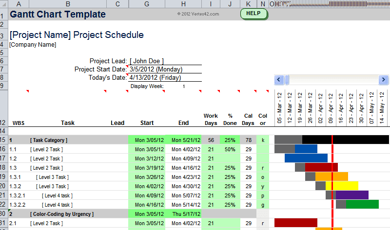
Gantt charts can be a bit old-school as agile project management methods are increasing in popularity, they are still being used widely. There are several Gantt chart excel templates on the web.
A Gantt chart example from vertex42.com:
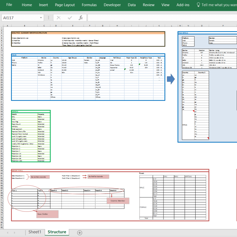
I just found out a reporting structure mockup I have prepared in Excel once upon a time:
By the way, did you see our Automatic Organization Chart Generator?
This is an Excel template that lets you create organization charts from Excel lists with a click of a button. It can be useful for small business owners and Human Resources departments.
These type of charts are directly related to Excel as most of the companies already keep their data in spreadsheets. But I also know people who even build their website mockups in Excel (with links to other sections, placement of buttons, sliders etc.).
Sometimes you may need your excel files to be updated automatically from a live data source. For example, if you are making a stock market analysis and want the latest data of some stock prices at NYSE, you can connect your Excel file to a data feed and let it take the latest info automatically (unless you want to input them one by one!)
As this is a comprehensive topic I will leave it for another post. But here is a few things you can fetch into excel:
- Stock prices
- Match results of soccer, NBA, NFL or any sports games (from live score sites)
- Fx rates
- Real-time flight data of airports
- Any info in a shared database (whether it is your company intranet or public)
This topic is getting more and more important as most data is kept on cloud systems. We don’t download info bits to our computers as we used to do in the past. So, Microsoft is working hard to improve the web integration of Excel.
Recommended Reading: Can Excel Extract Data From Website?
Yes, it is not the best idea to use Excel as a database. Because it is not designed for this purpose. Queries will take a long time especially when data gets bigger. It can be unreliable sometimes and not very secure. It is all accepted. However, we are not always after a complete set of the database systems and it can serve us as a mini-warehouse for our little data.

For example, if you keep records of your invoice data and want to make some sales analysis, it can be a good starting point. If later, you want to see more details, want to record more breakdowns you will need to move to a “real database”. It can be Access, SQL or anything. Just keep an eye on your Excel file because it has a maximum of 1 million rows.
Some of you may say “hey, it is more than enough, isn’t it?”
Generally yes. But you cannot believe how data increase in size when you want to see details. I remember when I was working as an analyst in a game development company, we were holding records of 1+ billion rows of data.
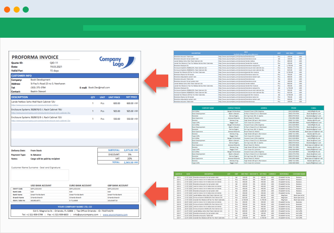
Precisely because of that, we have built some of our Excel templates (which is the favorite feature of all the users) with a database section. You may check our Invoice Generators and see how invoice recording would be super easy in Excel!
Conclusion
As the internet gets more available for everybody people started to use collaboration platforms more than before. In this aspect, online spreadsheet applications, like Google Sheets, increase in popularity and stands as a competitor to Microsoft’s Excel. Other free alternatives like open office or libre office are also popular. But if you need the advanced functionalities of Excel there is still no substitute.

Microsoft is improving the software actively. PowerPivot, Power BI, and Excel Online are all brand new features they developed recently. We will wait and see how things evolve in the following years. (investintech.com has made interviews with Excel experts about the future of Excel)
I tried to cover most of the things that can be done with Excel. If I have missed anything or if you find any errors, let me know by commenting down or sending an email.
Also, don’t forget to check our Excel Templates Collection. You may find something useful for yourself:
Excel Templates and Spreadsheets – Someka
Who said Excel takes lot of time / steps do something? Here is a list of 15 incredibly fun things you can do to your spreadsheets and each takes no more than 5 seconds to do.
Happy Friday 🙂
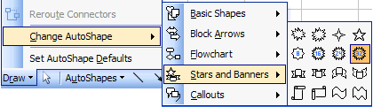
1. Change the shape / color of cell comments
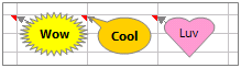
Just select the cell comment, go to draw menu in bottom left corner of the screen, and choose change auto shape option, select a 32 pointed star or heart symbol or a smiley face, just wow everyone 🙂
2. Filter unique items from a list
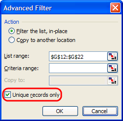
Select the data, go to data > filter > advanced filter and check the “unique items” option.
3. Sort from Left to Right
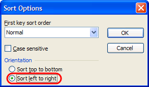
What if your data flows from left to right instead of top to bottom. Just change the sort orientation from “sort options” in the data > sort menu.
4. Hide the grid lines from your sheets
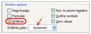
Go to Options dialog in tools menu, uncheck the “grid lines” option to remove gridlines from your worksheets. You can also change the color of grid line from here (not recommended)
5. Add rounded border to your charts, make them look smooth
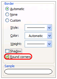
Just right click on the chart, select format chart option, in the dialog, check the “rounded borders”. You can even add a shadow effect from here.
6. Fetch live stock quotes / company research with one click
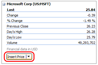
Just enter the stock symbol (MSFT, GOOG, AAPL etc.) in a cell, alt+click on the cell to launch “research pane”, select stock quotes to see MSN Money quotes for the selected symbol. You can fetch company profiles in the same way. Learn more.
7. Repeat rows on top when printing, show table headers on every page
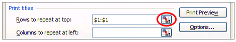
When you are on the sheet view, just hit menu > file > page setup, go to the last tab, specify “rows to repeat”. You can “repeat columns while printing” as well from the same menu.
8. Remove conditional formatting / all formatting with one click
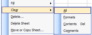
Just go to Menu > Edit > Clear > All to remove all the formatting from selected cell / range.
9. Auto sum cells with one click
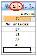
Select a bunch of cells and click on the Sigma symbol on the standard tool bar. Alternatively you can use Alt+= keyboard shortcut.
10. Find width of a column with formula, really!
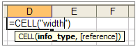
Just use =cell("width") to find the width of the column to which that formula cell belongs. Width is returned as the nearest integer.
11. Find total working days between any two dates, including holidays
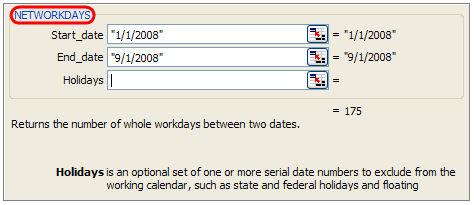
If you work on project plans, gantt charts alot, this can be totally handy. Just type =networkdays(start date, end date, list of holidays) to fetch the number of working days. In the above sample you can see the number of working days between New years day and September first of this year (labor day).
12. Freeze Rows / Columns in your sheet, Show important info even when scrolling
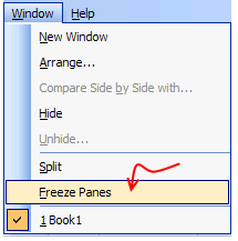
Select the cell diagonally beneath the row / columns you want to freeze (for eg. if you wan to freeze row 1&2 and columns A&B, click in C3), go to menu > window and click on freeze panes.
13. Split sheets in to two, compare side by side to be more productive
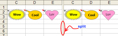
Just click on this little vertical bar on the bottom right corner of the sheet (see below) and drag it to create a vertical split. You can do the same way for a horizontal split as well 🙂

14. Change the color of various sheet name tabs
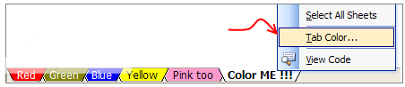
Right click on sheet and select “Tab color” option to change the worksheet tab colors. Group them with similar colors if you have lot of sheets, it looks nice.
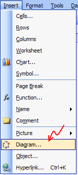
15. Insert a quick organization chart
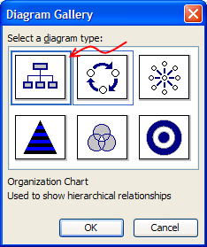
Click on menu > insert > diagram to open the above dialog, just select the organization chart option, enter node values and you have a pretty organization chart. Alternatively learn how to create org charts in excel.
So what do you say now? Isn’t Excel Exciting? 😀
Share this tip with your colleagues

Get FREE Excel + Power BI Tips
Simple, fun and useful emails, once per week.
Learn & be awesome.
-
121 Comments -
Ask a question or say something… -
Tagged under
cool, formatting, freeze panes, fun, how to, ideas, Learn Excel, microsoft, Microsoft Excel Formulas, spreadsheet, technology, tips, tricks
-
Category:
All Time Hits, Featured, hacks, ideas, Learn Excel

Welcome to Chandoo.org
Thank you so much for visiting. My aim is to make you awesome in Excel & Power BI. I do this by sharing videos, tips, examples and downloads on this website. There are more than 1,000 pages with all things Excel, Power BI, Dashboards & VBA here. Go ahead and spend few minutes to be AWESOME.
Read my story • FREE Excel tips book


Excel School made me great at work.
5/5

From simple to complex, there is a formula for every occasion. Check out the list now.

Calendars, invoices, trackers and much more. All free, fun and fantastic.

Power Query, Data model, DAX, Filters, Slicers, Conditional formats and beautiful charts. It’s all here.

Still on fence about Power BI? In this getting started guide, learn what is Power BI, how to get it and how to create your first report from scratch.
Related Tips
121 Responses to “Excel can be Exciting – 15 fun things you can do with your spreadsheet in less than 5 seconds”
-
Great tips! Another good one is highlighting a bunch of cells and changing the autosum visual at the bottom right to be Average or Count instead of auto sum.
-
[…] from a list, sorting data from left to right, freezing panes, and coloring your worksheet tabs. Excel can be Exciting : 15 Fun things to do with Microsoft Excel [Pointy Haired Dilbert — […]
-
[…] from a list, sorting data from left to right, freezing panes, and coloring your worksheet tabs. Excel can be Exciting : 15 Fun things to do with Microsoft Excel [Pointy Haired Dilbert — […]
-
 Adam says:
 one note on the «unique items» tip — this only works with numerical data — if you’re looking to weed out unique text entries, no dice — I work in Excel a lot with names and proprietary tags and would love a way to select a unique text entry — any suggestions?
-
badOedipus says:
You can filter duplicate text entries as described above if you use the advanced filter option, however it will not allow you to do an additional filter on an adjacent column afterwards without duplicating the data first.
The method detailed below will allow you to filter our duplicate entries based on a conditional format.Select the range from which you wish to filter out duplicate text entries
Click on Conditional Formatting > New Rule… > Use a formula to determine which cells to format
type the following formula in the text box: =AND(COUNTIF(«RangeAddress«, «FirstCellAddress«)>1, MATCH(«FirstCellAddress«,»RangeAddress«, 0)<> ROW()) making sure to substitute accordingly. Note: RangeAddress should be absolute(«$A$1:$A$20»), and FirstCellAddress should be relative («A1»).
Set the format to fill the cells with a color, depending on the application I use either a faint off-white to down play the color or a bright yellow to really make it pop — the choice is yours.
Ta-da your duplicates are now colored. You can now filter by color if you use 2010 to see only duplicates or only unique records (unique being only one record per value). Pre-2010 you can sort by color to get them at the top/bottom of your list. -
Adrian says:
Maybe if you use Access.
-
Vincent says:
First post on chandoo.org, wahoooo!
Anyways, after reading the above comments I just realized there’s a similar way to flag duplicate values with a formula, and one that works for strings as well as numbers. If you’re working in column A with a header row then your IDs will be in cells A2:A___. The following formula can be entered in B2 and filled downward to return FALSE when the ID is a repeated value, i.e. it is not the first instance of that value:
«=MATCH(A2,$A$2:$A$__,0)=(ROW(A2)-ROW($A$1))».-
Martin says:
Re: =MATCH(A2,$A$2:$A$__,0)=(ROW(A2)-ROW($A$1))
That’s a brilliant formula — I shall use that.
Many thanks for sharing!
-
-
-
Jason C says:
Just highlight duplicates and then filter out the highlighted cells.
-
-
Mazy says:
OK, my hint, I think this excel function have never been documented or referred even in manuals:)
If you want to insert a part of a worksheet as picture (e.g. you want to include a small chart to a preformatted excel document), do the following:
DRAW anything, a square, circle, etc.
SELECT the cells you want to insert as a picture
SELECT the object you made (square,etc.)
PASTEVoila:)
-
PK says:
I can’t get the comment to change. It just wants to draw a new autoshape.
-
Tom says:
To change the shape of the comment In Excel 2010 — I had to Customize the Ribbon [FILE, OPTIONS] and add a «Format» tab to the Main Tabs to allow the Format tab to be available all the time. Now I can Edit the shape.
-
-
@Adam.. It works for text data for me, which version of excel you are using, all these tips are tested in Excel 2003.
@PK … when you select comment to edit (shift+f2) click on the border of the comment, then go to bottom left corner in the screen and select draw > change auto shape. Should work in excel 2003 and above. Let me know if you see some problems 🙂
-
Renate Callahan says:
nope, it still doesn’t work. There is no draw -> change auto shape available for me. The left bottom corner of the screen just shows ‘Ready’ and if I right click on it it shows a lot of other things to activate, none of it is Draw or Auto options. I use Excel 2007
-
-
MM says:
You’ve missed an important step in your first tip. The Drawing toolbar must be active for this to work. Mine is not on by default, so I have to take the extra set to turn it on.
-
Jason says:
Very nice, thanks!
Could you clarify «You can also change the color of grid line from here (not recommended)» What is the recommended method.
-
The graphic designer-side of my job hates Excel, but the business owner side of me finds it to be essential. These tips help bring both sides (designer / business owner) closer together. Thanks!
-
@MM.. you are right, I have assumed the draw toolbar is on… thanks for pointing it out.
@Jason… “You can also change the color of grid line from here (not recommended)”, I said that to convey changing grid line colors is not recommended, as it can scare people or otherwise make your sheet look extremely busy… but you can change the color if you wish.. 😀
-
I use the NETWORKDAYS function all the time and it just blows people away.
-
Dude,
networkdays is my fav.🙂
Nice post.-Nikhil
-
My favorite excel command Ctrl and ~
displays all formulas -
Thanks you pointy haired Dilbert, this is definitely a great list, like always bookmarked for future uses 😀
-
greats tips
i like command for displaying all formulas
thanks -
Wade says:
Great tips!
However, #14 You need to right-click on the tab not the sheet.
#10 You can just left click and hold on the right most line of the column letter. Also, another tip a lot of users don’t know is that you can change a section of columns you want to one width by highlighting a column with the width you prefer and left-click-hold on the bottom right corner of that column letter and drag it through as many columns as you need. -
Excel can be Exciting : 15 Fun things to do with Microsoft Excel | Pointy Haired Dilbert — Chandoo.o…
Who said Excel takes lot of time steps do something Here is a list of 15 incredibly fun things you can do to your spreadsheets and each takes no more than 5…
-
hey says:
Great history class. Should have gone for Excel 97 while you were at it 😉
-
0751firewire says:
Hey, HEY
Don’t be rude. It’s a waste of everyone’s time — including yours. Totally unnecessary.
******
Thanks for this post! I really enjoyed reading these tips. I will bookmark this post and will also subscribe to your weekly newsletter!Thanks so much.
-
@Wade: you are right, you have to click on sheet name and not on sheet
and #10 was meant to show another way to find column width, but yeah, I always use the left click hold technique to see if the width is enough for me. Thanks for sharing it with everyone 🙂
@0751firewire: thanks 🙂
@everyone… I am happy so many of you liked this post and enjoyed these small but very useful stuff hidden away in the Excel.
-
LEO DA VINCI says:
Dear Chandoo,
I have discovered you only 3 days back . I want a help from you . I am using a software which makes a grid file of lat,long and elevn. data (x,y,z) on 25m into 25m mesh size . I feel that this grid file which is made from a xcel csv sheet containing random x,y,z points can be made on xcel sheet itself. Can i do that ? example of a source data shown belowx y z
100 50 12.5
200 40 14.0
220 75 12.0
202 60 15.0-
@Leo Da Vinci
You can either import and existing CSV file or setup the file directly in Excel as a workbook -
whatever says:
You can not make a grid gragh on xeel because it has boxes you would have too get speacial advanced software like the sciencestes do:
i know more that somebody from the GEEK squad!!
-
@Whatever
Can you post a sample of a Grid Graph or a link where we can see what your referring to?
-
-
-
-
[…] Excel can be Exciting : 15 Fun things to do with Microsoft Excel | Pointy Haired Dilbert — Chandoo.o… […]
-
Tip #13: In case anyone is an excel newbie like me, to remove the new vertical bar, just double click on the bar.
-
Rufus says:
Thanks fir the tip re vertical bar.
I am a baby Excel beginner at 86!!!!!
-
-
Roger says:
Unique text entries can be found easily — use COUNTIF function for each row. You can use autofilter to delete anything with result > 1.
-
LD says:
To the person joking about Excel 97 — that version of Office is still the standard at my workplace. No joke.
-
[…] Excel can be Exciting : 15 Fun things to do with Microsoft Excel | Pointy Haired Dilbert — Chandoo.o… […]
-
shivshankar says:
Adv
-
[…] Find total working days between any two dates, including holidays […]
-
Arti says:
I tried second tip to remove the duplicate entries from the row by copying it in another location but its not working if I use data in A’ th column as
A1 aa
A2 aa
A3 bband I am trying to copy the unique records to column B.
The above scenario is not working if duplicate entries are present in A1 and A2.
It will work if duplicate entries are present below first record. -
Robert says:
@Arti
Autofilter as well as advanced filter needs titles of the columns in the first row. If you have only the three items in your list, Excel assumes, the first «aa» is the title (field name) of your list, not an entry in the list itself. As a result, Excel writes into column B again the first aa as the title and the second aa and bb as the 2 entires.
Simply insert a row above your list and give your list a name in cell A1. Then it should work.
-
[…] more than 5 seconds to do. Happy Friday 1. Change the shape / color of cell comments Just select thhttp://chandoo.org/wp/2008/08/01/15-fun-things-with-excel/MI-INFO Tutorials — Excel BasicsFor large worksheets that span more than one screen of […]
-
[…] Excel can be Exciting : 15 Fun things to do with Microsoft Excel […]
-
[…] on September 13, 2008 Few weeks back, I came across a post about some useful tips in MS Excel — Excel can be exciting . So, I thought I’ll collate some of the helpful tips and tricks that I’ve come across while […]
-
[…] 15 Fun things you can do with Excel […]
-
Melli says:
Nr. 5
-> does not work. And I have Excel 2003! -
@Melli .. Welcome to PHD…
Are you sure rounded borders are not working. I have made this example in Excel 2003 and they are working alright for me. You have to select the entire chart to change borders to rounded, not the plot area alone.
-
[…] Excel can be Exciting : 15 Fun things to do with Microsoft Excel | Pointy Haired Dilbert — Chandoo.o… (tags: work windows useful tutorials tutorial tricks toread tools) […]
-
[…] But often we leave the last steps for manual processing. The article addresses one such problem (extracting unique cells from a range) and tells us how we can automate the whole […]
-
homepage templates…
I just wanted to share this nice address, where you can get wordpress themes for free. I use one of the designs for my own blog and it was really easy to install. Just activating it in admin and the job was done. :-)…
-
I did not know excel is this much fun.
-
Ketan says:
@ Adam & Chandoo…
For removing / filtering the duplicate entry / unique data…one can use the readymade menu from JMT utilities….very useful… -
[…] Using Advanced Data Filter […]
-
[…] Excel can be Exciting — 15 fun things you can do with excel […]
-
rayna says:
Thx so much PHD…tusi gr8 ho ji…:)
-
[…] > and un-check grid lines option. (Excel 2007: office button > excel option > advanced)… Get Full Tip 50. To hide a worksheet, go to menu > format > sheet > hide… Get Full Tip 51. To align […]
-
[…] Beautiful City Photography» and «10 Companies Hiring for Work from Home». (They’ve also included «15 fun things to do with Microsoft Excel», which may be the most terrifying title in blogging […]
-
[…] Learn Excel Formulas in Plain English | Executive Dashboards in Excel — 4 Part Tutorial | 15 Excel Fun Tips […]
-
[…] Related: How to change the shape of cell comments from rectangle to any other shape […]
-
[…] Learn how to color excel worksheet tabs. […]
-
[…] on excel comments: change the shape of excel comment box | pimp your comment boxes | extract comments using […]
-
Francis says:
i cannot find CHANGE AUTO SHAPE option in Excel 2007 to design my comment box. Please help?
-
@Francis… Excel 2007 has made it little difficult to change comment shapes, but it is still possible. First add a regular shape (like rectangle) to the worksheet. Now select it. This will show a new ribbon called «format». From here, you can find the change shape tool. Add this tool to Quick Access Bar.
Now Select the comment cell and edit comment. At this point, use the change shape tool from QAT to change the shape of comment.
-
Renate Callahan says:
all right!! Thanks, this answers my question posted above. Yes, now it does work and it looks great! 🙂
-
-
-
Ken Buffong says:
Its really made easy.
-
Paul says:
Its a bit of a faff in 2007, not sure if its just my work computer than won’t let me change the default shape for comment boxes… But for this one workbook i’ve added a simple:
ActiveCell.Comment.Shape.Select
Selection.ShapeRange.AutoShapeType = msoShapeVerticalScrollOr you can change msoShapeVeriticalScroll to any shape you like…
-
VENKATRAMAN V S says:
Dear All
Thank you all very much. You guys have taught me a lot of new things in Excel. Keep continuing the good work.
-
nazia says:
thanx so much…it really is of gr8 gr8 help to me…… :))
-
The color sheet tab option has disappeared. Was there and working fine but now when I right click there isn’t an option to change the color of my sheets. How can I get this option back?
-
@Deanna.. you can reach this from Format button on home ribbon. Key board short code — ALT + HOT (just press h,o and t one after another).
-
-
Sanjay says:
Hello,
Can I know the name of the last person who saved the file last.
In a team of 10 members working on a shared excel file, this information will help me to know the name of the person who modified the file.
-
Shouvik says:
@Sanjay: Open the workbook — Click on File -> Properties -> Click on the Statistics Tab for the information you are looking for.
-
mer says:
Wish I could see those images, because they’re now blocked by photobucket. Next time use imgur, or host it on your own server.
-
mimi says:
Brilliant!
Helped me teach my pupils loads in I.C.T today!
LOL -
irha says:
you don’t have references 🙁
-
Hussein says:
I liked a lot this web site
thanks
-
Rahul aggarwal says:
@chandoo ji
can we change default comment cell box shape in excel 2007or 2010? -
saravanan says:
Hi Friends
Can we Increase the Column width >500 in excel 2003.
Pls help…
-
losraiders says:
I really like tip #1 but I’m how can you do it if you’re using Excel 2007. I don’t see the drawing toolbar…I believe it’s gone in 2007 but not certain. I did see the autoshape when I select the commnent and right click but nothing happens when I select it.
-
This is possible in Excel 2007 (and 2010) too. Follow below steps:
- Add any drawing shape.
- Select it and go to format ribbon
- Right click on Edit shape and add it to «Quick Access toolbar»
- Now, remove the shape
- Select comment cell.
- Edit comment.
- Use quick access toolbar to change the shape to anything you want.
-
Sudhir says:
This is awesome Chandoo ! Tip#1 I was most impressed. #6 I was not able to replicate — if you meant Alt + (Mouse left) click, it did not work. But manually triggered the reference — but was unable again to make it available as embedded «auto look up» in the sheet itself.
-
-
steve says:
wow! this site is awesome
-
Some tricks are not working with Excel 2003
But others are too cool thanx
-
[…] and un-check grid lines option. (Excel 2007: office button > excel option > advanced)… Get Full Tip 50. To hide a worksheet, go to menu > format > sheet > hide… Get Full Tip 51. To […]
-
[…] Using too many tab colors on your excel workbooks [how to do this] […]
-
Can anyone help. I want to be able to hide a row for exampe row A if the Cell A1 is empty after i have sorted the rows.
I can write the macro to sort the list then I am stuck.Any HELP OUT THERE.
Regards ken
-
why isnt my thing working
=NETWORKDAYS(«11/11/2011″,»12/12/2012»,[holidays])-
D Gamlath says:
It’s not going to work that way. At least not with the parentheses. Try entering the two dates in two cells and referring those cells within your formula 🙂
-
Sudhir says:
It will work — a date in formula is entered as follows:
=NETWORKDAYS(DATE(2011,11,11),DATE(2012,12,12),0)
-
-
Marcia Fay Cobb says:
I’m doing an address directory. All I want to do is find out how to delete a blank line or move the second line up to the first line in the cell? Appreciate any help you can give. Thanks.
-
Shivani says:
How to make comments of different shapes in Excel 2010?
-
Jignesh says:
we have shared the workbook, so other user can access and feed data at their respective fields, all user can view list of users accessing the shared file,but unfortunately if a user removed from list of user name then that user will be disconnected and whatever changes made will be proved to be useless as file become exclusive.
Could you please anybody help me out how to protect the username list so nobody could removed from the list.
-
Abdul Azeez says:
how to change font color in cell by using formula
-
Sudhir says:
This can be done using conditional formatting. Is there a specific thing that you are looking at ?
-
-
Nadalvski says:
Hi Chandoo,
I bumped into your site two days ago and am hooked to it.
Very helpful and elaborate articles.
Thanks. -
[…] Check out why here. […]
-
Prakash says:
Can anyone help me to do the following:
Is there any option to copy all the procedures done for a set of values to other set of value which we will input in later stages.
In other words: Imagine I have a list of values(first set) for which I need to do some mathematical and logical operations and I will get the final required output.Also if I have one more set of values(second set) for which I need to do the same procedure to get required output.
So my question is : Is there any way to get the final output directly for set-2 values based on the steps(procedures) done for set-1 so that it will reduce lot of work.Please help me.
Thank you all.-
@Prakash
Can you ask the question in the forums
http://chandoo.org/forum/
Please also attach a sample file with an example of what results you want
-
-
nmsdfmn says:
whey it is appearing
-
Kris says:
I think you should mention that this feature available from WHAT Version otherwise users go crazy!
-
extreme x says:
Oh very cool stuff! Thanks
-
Rushabh Gala says:
This is really a good article even I read some comments which were really useful.
-
Chirag Parmar says:
That was cool Sir. Thanks for sharing these tricks with us.
-
Dustin says:
Help!! I just pulled data out of a different software and pasted values only in excel. Anything with a character other than a number is shifted to the left of the cell. Anything with only numbers is shifted to the right of the cell.
The VLOOKUP is only working on the ones shifted to the right. The formatting on the home tab is all the same. Why is it working on some but not the others? Is there underlying format that can be erased??
-
Dustin says:
The VLOOKUP is only working on the ones shifted to the left.********
(Only works for cells that have characters other than numbers, in addition to numbers)
-
-
thanks for your tips and tutorials excel for children… i like
-
sandeep kothari says:
Hat tip to you, OSUM Chandoo!
-
Sandy says:
I’m adding birthdates to a column. I need to know how to differentiate a birthdate in the 19 hundreds (19XX) from a birthdate in the 2 thousands (20XX).
I appreciate any help!!! Thank you
-
Chad Estes says:
Assuming your birth date column is G and is a date datatype:
=if(YEAR(G1) < 2000, «Born in 20th Century», «Born in 21st Century»)
-
Sagar says:
Is there any way that, I can overlap and compare between two worksheets. This is required in case to auto highlight edited data between the copies. Please help….
-
Nice post . Step -> 7. Repeat rows on top when printing, show table headers on every page — will be useful . Thank you.
-
Bhanu Prasad K S says:
Hi Chandoo,
Firstly, I wanted to say a big thank you for whatever you are doing for people like me who need knowledge of excel and power BI.
I wanted to know how we can highlight cells which have dates between the given range.
for example, i want to highlight cell which have dates between Jan 1, 2022 and June 30, 2022.
Leave a Reply
Sometimes, Excel seems too good to be true. All I have to do is enter a formula, and pretty much anything I’d ever need to do manually can be done automatically.
Need to merge two sheets with similar data? Excel can do it.
Need to do simple math? Excel can do it.
Need to combine information in multiple cells? Excel can do it.
In this post, I’ll go over the best tips, tricks, and shortcuts you can use right now to take your Excel game to the next level. No advanced Excel knowledge required.
![Download 10 Excel Templates for Marketers [Free Kit]](https://no-cache.hubspot.com/cta/default/53/9ff7a4fe-5293-496c-acca-566bc6e73f42.png)
-
What is Excel?
-
Excel Basics
-
How to Use Excel
-
Excel Tips
-
Excel Keyboard Shortcuts
What is Excel?
Microsoft Excel is powerful data visualization and analysis software, which uses spreadsheets to store, organize, and track data sets with formulas and functions. Excel is used by marketers, accountants, data analysts, and other professionals. It’s part of the Microsoft Office suite of products. Alternatives include Google Sheets and Numbers.
Find more Excel alternatives here.
What is Excel used for?
Excel is used to store, analyze, and report on large amounts of data. It is often used by accounting teams for financial analysis, but can be used by any professional to manage long and unwieldy datasets. Examples of Excel applications include balance sheets, budgets, or editorial calendars.
Excel is primarily used for creating financial documents because of its strong computational powers. You’ll often find the software in accounting offices and teams because it allows accountants to automatically see sums, averages, and totals. With Excel, they can easily make sense of their business’ data.
While Excel is primarily known as an accounting tool, professionals in any field can use its features and formulas — especially marketers — because it can be used for tracking any type of data. It removes the need to spend hours and hours counting cells or copying and pasting performance numbers. Excel typically has a shortcut or quick fix that speeds up the process.
You can also download Excel templates below for all of your marketing needs.
After you download the templates, it’s time to start using the software. Let’s cover the basics first.
Excel Basics
If you’re just starting out with Excel, there are a few basic commands that we suggest you become familiar with. These are things like:
- Creating a new spreadsheet from scratch.
- Executing basic computations like adding, subtracting, multiplying, and dividing.
- Writing and formatting column text and titles.
- Using Excel’s auto-fill features.
- Adding or deleting single columns, rows, and spreadsheets. (Below, we’ll get into how to add things like multiple columns and rows.)
- Keeping column and row titles visible as you scroll past them in a spreadsheet, so that you know what data you’re filling as you move further down the document.
- Sorting your data in alphabetical order.
Let’s explore a few of these more in-depth.
For instance, why does auto-fill matter?
If you have any basic Excel knowledge, it’s likely you already know this quick trick. But to cover our bases, allow me to show you the glory of autofill. This lets you quickly fill adjacent cells with several types of data, including values, series, and formulas.
There are multiple ways to deploy this feature, but the fill handle is among the easiest. Select the cells you want to be the source, locate the fill handle in the lower-right corner of the cell, and either drag the fill handle to cover cells you want to fill or just double click:
 Similarly, sorting is an important feature you’ll want to know when organizing your data in Excel.
Sometimes you may have a list of data that has no organization whatsoever. Maybe you exported a list of your marketing contacts or blog posts. Whatever the case may be, Excel’s sort feature will help you alphabetize any list.
Click on the data in the column you want to sort. Then click on the «Data» tab in your toolbar and look for the «Sort» option on the left. If the «A» is on top of the «Z,» you can just click on that button once. If the «Z» is on top of the «A,» click on the button twice. When the «A» is on top of the «Z,» that means your list will be sorted in alphabetical order. However, when the «Z» is on top of the «A,» that means your list will be sorted in reverse alphabetical order.
Let’s explore more of the basics of Excel (along with advanced features) next.
To use Excel, you only need to input the data into the rows and columns. And then you’ll use formulas and functions to turn that data into insights.
We’re going to go over the best formulas and functions you need to know. But first, let’s take a look at the types of documents you can create using the software. That way, you have an overarching understanding of how you can use Excel in your day-to-day.
Documents You Can Create in Excel
Not sure how you can actually use Excel in your team? Here is a list of documents you can create:
- Income Statements: You can use an Excel spreadsheet to track a company’s sales activity and financial health.
- Balance Sheets: Balance sheets are among the most common types of documents you can create with Excel. It allows you to get a holistic view of a company’s financial standing.
- Calendar: You can easily create a spreadsheet monthly calendar to track events or other date-sensitive information.
Here are some documents you can create specifically for marketers.
- Marketing Budgets: Excel is a strong budget-keeping tool. You can create and track marketing budgets, as well as spend, using Excel. If you don’t want to create a document from scratch, download our marketing budget templates for free.
- Marketing Reports: If you don’t use a marketing tool such as Marketing Hub, you might find yourself in need of a dashboard with all of your reports. Excel is an excellent tool to create marketing reports. Download free Excel marketing reporting templates here.
- Editorial Calendars: You can create editorial calendars in Excel. The tab format makes it extremely easy to track your content creation efforts for custom time ranges. Download a free editorial content calendar template here.
- Traffic and Leads Calculator: Because of its strong computational powers, Excel is an excellent tool to create all sorts of calculators — including one for tracking leads and traffic. Click here to download a free premade lead goal calculator.
This is only a small sampling of the types of marketing and business documents you can create in Excel. We’ve created an extensive list of Excel templates you can use right now for marketing, invoicing, project management, budgeting, and more.
In the spirit of working more efficiently and avoiding tedious, manual work, here are a few Excel formulas and functions you’ll need to know.
Excel Formulas
It’s easy to get overwhelmed by the wide range of Excel formulas that you can use to make sense out of your data. If you’re just getting started using Excel, you can rely on the following formulas to carry out some complex functions — without adding to the complexity of your learning path.
- Equal sign: Before creating any formula, you’ll need to write an equal sign (=) in the cell where you want the result to appear.
- Addition: To add the values of two or more cells, use the + sign. Example: =C5+D3.
- Subtraction: To subtract the values of two or more cells, use the — sign. Example: =C5-D3.
- Multiplication: To multiply the values of two or more cells, use the * sign. Example: =C5*D3.
- Division: To divide the values of two or more cells, use the / sign. Example: =C5/D3.
Putting all of these together, you can create a formula that adds, subtracts, multiplies, and divides all in one cell. Example: =(C5-D3)/((A5+B6)*3).
For more complex formulas, you’ll need to use parentheses around the expressions to avoid accidentally using the PEMDAS order of operations. Keep in mind that you can use plain numbers in your formulas.
Excel Functions
Excel functions automate some of the tasks you would use in a typical formula. For instance, instead of using the + sign to add up a range of cells, you’d use the SUM function. Let’s look at a few more functions that will help automate calculations and tasks.
- SUM: The SUM function automatically adds up a range of cells or numbers. To complete a sum, you would input the starting cell and the final cell with a colon in between. Here’s what that looks like: SUM(Cell1:Cell2). Example: =SUM(C5:C30).
- AVERAGE: The AVERAGE function averages out the values of a range of cells. The syntax is the same as the SUM function: AVERAGE(Cell1:Cell2). Example: =AVERAGE(C5:C30).
- IF: The IF function allows you to return values based on a logical test. The syntax is as follows: IF(logical_test, value_if_true, [value_if_false]). Example: =IF(A2>B2,»Over Budget»,»OK»).
- VLOOKUP: The VLOOKUP function helps you search for anything on your sheet’s rows. The syntax is: VLOOKUP(lookup value, table array, column number, Approximate match (TRUE) or Exact match (FALSE)). Example: =VLOOKUP([@Attorney],tbl_Attorneys,4,FALSE).
- INDEX: The INDEX function returns a value from within a range. The syntax is as follows: INDEX(array, row_num, [column_num]).
- MATCH: The MATCH function looks for a certain item in a range of cells and returns the position of that item. It can be used in tandem with the INDEX function. The syntax is: MATCH(lookup_value, lookup_array, [match_type]).
- COUNTIF: The COUNTIF function returns the number of cells that meet a certain criteria or have a certain value. The syntax is: COUNTIF(range, criteria). Example: =COUNTIF(A2:A5,»London»).
Okay, ready to get into the nitty-gritty? Let’s get to it. (And to all the Harry Potter fans out there … you’re welcome in advance.)
Excel Tips
- Use Pivot tables to recognize and make sense of data.
- Add more than one row or column.
- Use filters to simplify your data.
- Remove duplicate data points or sets.
- Transpose rows into columns.
- Split up text information between columns.
- Use these formulas for simple calculations.
- Get the average of numbers in your cells.
- Use conditional formatting to make cells automatically change color based on data.
- Use IF Excel formula to automate certain Excel functions.
- Use dollar signs to keep one cell’s formula the same regardless of where it moves.
- Use the VLOOKUP function to pull data from one area of a sheet to another.
- Use INDEX and MATCH formulas to pull data from horizontal columns.
- Use the COUNTIF function to make Excel count words or numbers in any range of cells.
- Combine cells using ampersand.
- Add checkboxes.
- Hyperlink a cell to a website.
- Add drop-down menus.
- Use the format painter.
Note: The GIFs and visuals are from a previous version of Excel. When applicable, the copy has been updated to provide instruction for users of both newer and older Excel versions.
1. Use Pivot tables to recognize and make sense of data.
Pivot tables are used to reorganize data in a spreadsheet. They won’t change the data that you have, but they can sum up values and compare different information in your spreadsheet, depending on what you’d like them to do.
Let’s take a look at an example. Let’s say I want to take a look at how many people are in each house at Hogwarts. You may be thinking that I don’t have too much data, but for longer data sets, this will come in handy.
To create the Pivot Table, I go to Data > Pivot Table. If you’re using the most recent version of Excel, you’d go to Insert > Pivot Table. Excel will automatically populate your Pivot Table, but you can always change around the order of the data. Then, you have four options to choose from.
- Report Filter: This allows you to only look at certain rows in your dataset. For example, if I wanted to create a filter by house, I could choose to only include students in Gryffindor instead of all students.
- Column Labels: These would be your headers in the dataset.
- Row Labels: These could be your rows in the dataset. Both Row and Column labels can contain data from your columns (e.g. First Name can be dragged to either the Row or Column label — it just depends on how you want to see the data.)
- Value: This section allows you to look at your data differently. Instead of just pulling in any numeric value, you can sum, count, average, max, min, count numbers, or do a few other manipulations with your data. In fact, by default, when you drag a field to Value, it always does a count.
Since I want to count the number of students in each house, I’ll go to the Pivot table builder and drag the House column to both the Row Labels and the Values. This will sum up the number of students associated with each house.
2. Add more than one row or column.
As you play around with your data, you might find you’re constantly needing to add more rows and columns. Sometimes, you may even need to add hundreds of rows. Doing this one-by-one would be super tedious. Luckily, there’s always an easier way.
To add multiple rows or columns in a spreadsheet, highlight the same number of preexisting rows or columns that you want to add. Then, right-click and select «Insert.»
In the example below, I want to add an additional three rows. By highlighting three rows and then clicking insert, I’m able to add an additional three blank rows into my spreadsheet quickly and easily.
3. Use filters to simplify your data.
When you’re looking at very large data sets, you don’t usually need to be looking at every single row at the same time. Sometimes, you only want to look at data that fit into certain criteria.
That’s where filters come in.
Filters allow you to pare down your data to only look at certain rows at one time. In Excel, a filter can be added to each column in your data — and from there, you can then choose which cells you want to view at once.
Let’s take a look at the example below. Add a filter by clicking the Data tab and selecting «Filter.» Clicking the arrow next to the column headers and you’ll be able to choose whether you want your data to be organized in ascending or descending order, as well as which specific rows you want to show.
In my Harry Potter example, let’s say I only want to see the students in Gryffindor. By selecting the Gryffindor filter, the other rows disappear.
 Pro Tip: Copy and paste the values in the spreadsheet when a Filter is on to do additional analysis in another spreadsheet.
4. Remove duplicate data points or sets.
Larger data sets tend to have duplicate content. You may have a list of multiple contacts in a company and only want to see the number of companies you have. In situations like this, removing the duplicates comes in quite handy.
To remove your duplicates, highlight the row or column that you want to remove duplicates of. Then, go to the Data tab and select «Remove Duplicates» (which is under the Tools subheader in the older version of Excel). A pop-up will appear to confirm which data you want to work with. Select «Remove Duplicates,» and you’re good to go.
You can also use this feature to remove an entire row based on a duplicate column value. So if you have three rows with Harry Potter’s information and you only need to see one, then you can select the whole dataset and then remove duplicates based on email. Your resulting list will have only unique names without any duplicates.
5. Transpose rows into columns.
When you have rows of data in your spreadsheet, you might decide you actually want to transform the items in one of those rows into columns (or vice versa). It would take a lot of time to copy and paste each individual header — but what the transpose feature allows you to do is simply move your row data into columns, or the other way around.
Start by highlighting the column that you want to transpose into rows. Right-click it, and then select «Copy.» Next, select the cells on your spreadsheet where you want your first row or column to begin. Right-click on the cell, and then select «Paste Special.» A module will appear — at the bottom, you’ll see an option to transpose. Check that box and select OK. Your column will now be transferred to a row or vice-versa.
On newer versions of Excel, a drop-down will appear instead of a pop-up.

6. Split up text information between columns.
What if you want to split out information that’s in one cell into two different cells? For example, maybe you want to pull out someone’s company name through their email address. Or perhaps you want to separate someone’s full name into a first and last name for your email marketing templates.
Thanks to Excel, both are possible. First, highlight the column that you want to split up. Next, go to the Data tab and select «Text to Columns.» A module will appear with additional information.
First, you need to select either «Delimited» or «Fixed Width.»
- «Delimited» means you want to break up the column based on characters such as commas, spaces, or tabs.
- «Fixed Width» means you want to select the exact location on all the columns that you want the split to occur.
In the example case below, let’s select «Delimited» so we can separate the full name into first name and last name.
Then, it’s time to choose the Delimiters. This could be a tab, semi-colon, comma, space, or something else. («Something else» could be the «@» sign used in an email address, for example.) In our example, let’s choose the space. Excel will then show you a preview of what your new columns will look like.
When you’re happy with the preview, press «Next.» This page will allow you to select Advanced Formats if you choose to. When you’re done, click «Finish.»
7. Use formulas for simple calculations.
In addition to doing pretty complex calculations, Excel can help you do simple arithmetic like adding, subtracting, multiplying, or dividing any of your data.
- To add, use the + sign.
- To subtract, use the — sign.
- To multiply, use the * sign.
- To divide, use the / sign.
You can also use parentheses to ensure certain calculations are done first. In the example below (10+10*10), the second and third 10 were multiplied together before adding the additional 10. However, if we made it (10+10)*10, the first and second 10 would be added together first.
8. Get the average of numbers in your cells.
If you want the average of a set of numbers, you can use the formula =AVERAGE(Cell1:Cell2). If you want to sum up a column of numbers, you can use the formula =SUM(Cell1:Cell2).
9. Use conditional formatting to make cells automatically change color based on data.
Conditional formatting allows you to change a cell’s color based on the information within the cell. For example, if you want to flag certain numbers that are above average or in the top 10% of the data in your spreadsheet, you can do that. If you want to color code commonalities between different rows in Excel, you can do that. This will help you quickly see information that is important to you.
To get started, highlight the group of cells you want to use conditional formatting on. Then, choose «Conditional Formatting» from the Home menu and select your logic from the dropdown. (You can also create your own rule if you want something different.) A window will pop up that prompts you to provide more information about your formatting rule. Select «OK» when you’re done, and you should see your results automatically appear.
10. Use the IF Excel formula to automate certain Excel functions.
Sometimes, we don’t want to count the number of times a value appears. Instead, we want to input different information into a cell if there is a corresponding cell with that information.
For example, in the situation below, I want to award ten points to everyone who belongs in the Gryffindor house. Instead of manually typing in 10’s next to each Gryffindor student’s name, I can use the IF Excel formula to say that if the student is in Gryffindor, then they should get ten points.
The formula is: IF(logical_test, value_if_true, [value_if_false])
Example Shown Below: =IF(D2=»Gryffindor»,»10″,»0″)
In general terms, the formula would be IF(Logical Test, value of true, value of false). Let’s dig into each of these variables.
- Logical_Test: The logical test is the «IF» part of the statement. In this case, the logic is D2=»Gryffindor» because we want to make sure that the cell corresponding with the student says «Gryffindor.» Make sure to put Gryffindor in quotation marks here.
- Value_if_True: This is what we want the cell to show if the value is true. In this case, we want the cell to show «10» to indicate that the student was awarded the 10 points. Only use quotation marks if you want the result to be text instead of a number.
- Value_if_False: This is what we want the cell to show if the value is false. In this case, for any student not in Gryffindor, we want the cell to show «0». Only use quotation marks if you want the result to be text instead of a number.
Note: In the example above, I awarded 10 points to everyone in Gryffindor. If I later wanted to sum the total number of points, I wouldn’t be able to because the 10’s are in quotes, thus making them text and not a number that Excel can sum.
The real power of the IF function comes when you string multiple IF statements together, or nest them. This allows you to set multiple conditions, get more specific results, and ultimately organize your data into more manageable chunks.
Ranges are one way to segment your data for better analysis. For example, you can categorize data into values that are less than 10, 11 to 50, or 51 to 100. Here’s how that looks in practice:
=IF(B3<11,“10 or less”,IF(B3<51,“11 to 50”,IF(B3<100,“51 to 100”)))
It can take some trial-and-error, but once you have the hang of it, IF formulas will become your new Excel best friend.
11. Use dollar signs to keep one cell’s formula the same regardless of where it moves.
Have you ever seen a dollar sign in an Excel formula? When used in a formula, it isn’t representing an American dollar; instead, it makes sure that the exact column and row are held the same even if you copy the same formula in adjacent rows.
You see, a cell reference — when you refer to cell A5 from cell C5, for example — is relative by default. In that case, you’re actually referring to a cell that’s five columns to the left (C minus A) and in the same row (5). This is called a relative formula. When you copy a relative formula from one cell to another, it’ll adjust the values in the formula based on where it’s moved. But sometimes, we want those values to stay the same no matter whether they’re moved around or not — and we can do that by turning the formula into an absolute formula.
To change the relative formula (=A5+C5) into an absolute formula, we’d precede the row and column values by dollar signs, like this: (=$A$5+$C$5). (Learn more on Microsoft Office’s support page here.)
12. Use the VLOOKUP function to pull data from one area of a sheet to another.
Have you ever had two sets of data on two different spreadsheets that you want to combine into a single spreadsheet?
For example, you might have a list of people’s names next to their email addresses in one spreadsheet, and a list of those same people’s email addresses next to their company names in the other — but you want the names, email addresses, and company names of those people to appear in one place.
I have to combine data sets like this a lot — and when I do, the VLOOKUP is my go-to formula.
Before you use the formula, though, be absolutely sure that you have at least one column that appears identically in both places. Scour your data sets to make sure the column of data you’re using to combine your information is exactly the same, including no extra spaces.
The formula: =VLOOKUP(lookup value, table array, column number, Approximate match (TRUE) or Exact match (FALSE))
The formula with variables from our example below: =VLOOKUP(C2,Sheet2!A:B,2,FALSE)
In this formula, there are several variables. The following is true when you want to combine information in Sheet 1 and Sheet 2 onto Sheet 1.
- Lookup Value: This is the identical value you have in both spreadsheets. Choose the first value in your first spreadsheet. In the example that follows, this means the first email address on the list, or cell 2 (C2).
- Table Array: The table array is the range of columns on Sheet 2 you’re going to pull your data from, including the column of data identical to your lookup value (in our example, email addresses) in Sheet 1 as well as the column of data you’re trying to copy to Sheet 1. In our example, this is «Sheet2!A:B.» «A» means Column A in Sheet 2, which is the column in Sheet 2 where the data identical to our lookup value (email) in Sheet 1 is listed. The «B» means Column B, which contains the information that’s only available in Sheet 2 that you want to translate to Sheet 1.
- Column Number: This tells Excel which column the new data you want to copy to Sheet 1 is located in. In our example, this would be the column that «House» is located in. «House» is the second column in our range of columns (table array), so our column number is 2. [Note: Your range can be more than two columns. For example, if there are three columns on Sheet 2 — Email, Age, and House — and you still want to bring House onto Sheet 1, you can still use a VLOOKUP. You just need to change the «2» to a «3» so it pulls back the value in the third column: =VLOOKUP(C2:Sheet2!A:C,3,false).]
- Approximate Match (TRUE) or Exact Match (FALSE): Use FALSE to ensure you pull in only exact value matches. If you use TRUE, the function will pull in approximate matches.
In the example below, Sheet 1 and Sheet 2 contain lists describing different information about the same people, and the common thread between the two is their email addresses. Let’s say we want to combine both datasets so that all the house information from Sheet 2 translates over to Sheet 1.
So when we type in the formula =VLOOKUP(C2,Sheet2!A:B,2,FALSE), we bring all the house data into Sheet 1.
Keep in mind that VLOOKUP will only pull back values from the second sheet that are to the right of the column containing your identical data. This can lead to some limitations, which is why some people prefer to use the INDEX and MATCH functions instead.
13. Use INDEX and MATCH formulas to pull data from horizontal columns.
Like VLOOKUP, the INDEX and MATCH functions pull in data from another dataset into one central location. Here are the main differences:
- VLOOKUP is a much simpler formula. If you’re working with large data sets that would require thousands of lookups, using the INDEX and MATCH function will significantly decrease load time in Excel.
- The INDEX and MATCH formulas work right-to-left, whereas VLOOKUP formulas only work as a left-to-right lookup. In other words, if you need to do a lookup that has a lookup column to the right of the results column, then you’d have to rearrange those columns in order to do a VLOOKUP. This can be tedious with large datasets and/or lead to errors.
So if I want to combine information in Sheet 1 and Sheet 2 onto Sheet 1, but the column values in Sheets 1 and 2 aren’t the same, then to do a VLOOKUP, I would need to switch around my columns. In this case, I’d choose to do an INDEX and MATCH instead.
Let’s look at an example. Let’s say Sheet 1 contains a list of people’s names and their Hogwarts email addresses, and Sheet 2 contains a list of people’s email addresses and the Patronus that each student has. (For the non-Harry Potter fans out there, every witch or wizard has an animal guardian called a «Patronus» associated with him or her.) The information that lives in both sheets is the column containing email addresses, but this email address column is in different column numbers on each sheet. I’d use the INDEX and MATCH formulas instead of VLOOKUP so I wouldn’t have to switch any columns around.
So what’s the formula, then? The formula is actually the MATCH formula nested inside the INDEX formula. You’ll see I differentiated the MATCH formula using a different color here.
The formula: =INDEX(table array, MATCH formula)
This becomes: =INDEX(table array, MATCH (lookup_value, lookup_array))
The formula with variables from our example below: =INDEX(Sheet2!A:A,(MATCH(Sheet1!C:C,Sheet2!C:C,0)))
Here are the variables:
- Table Array: The range of columns on Sheet 2 containing the new data you want to bring over to Sheet 1. In our example, «A» means Column A, which contains the «Patronus» information for each person.
- Lookup Value: This is the column in Sheet 1 that contains identical values in both spreadsheets. In the example that follows, this means the «email» column on Sheet 1, which is Column C. So: Sheet1!C:C.
- Lookup Array: This is the column in Sheet 2 that contains identical values in both spreadsheets. In the example that follows, this refers to the «email» column on Sheet 2, which happens to also be Column C. So: Sheet2!C:C.
Once you have your variables straight, type in the INDEX and MATCH formulas in the top-most cell of the blank Patronus column on Sheet 1, where you want the combined information to live.
14. Use the COUNTIF function to make Excel count words or numbers in any range of cells.
Instead of manually counting how often a certain value or number appears, let Excel do the work for you. With the COUNTIF function, Excel can count the number of times a word or number appears in any range of cells.
For example, let’s say I want to count the number of times the word «Gryffindor» appears in my data set.
The formula: =COUNTIF(range, criteria)
The formula with variables from our example below: =COUNTIF(D:D,»Gryffindor»)
In this formula, there are several variables:
- Range: The range that we want the formula to cover. In this case, since we’re only focusing on one column, we use «D:D» to indicate that the first and last column are both D. If I were looking at columns C and D, I would use «C:D.»
- Criteria: Whatever number or piece of text you want Excel to count. Only use quotation marks if you want the result to be text instead of a number. In our example, the criteria is «Gryffindor.»
Simply typing in the COUNTIF formula in any cell and pressing «Enter» will show me how many times the word «Gryffindor» appears in the dataset.
15. Combine cells using &.
Databases tend to split out data to make it as exact as possible. For example, instead of having a column that shows a person’s full name, a database might have the data as a first name and then a last name in separate columns. Or, it may have a person’s location separated by city, state, and zip code. In Excel, you can combine cells with different data into one cell by using the «&» sign in your function.
The formula with variables from our example below: =A2&» «&B2
Let’s go through the formula together using an example. Pretend we want to combine first names and last names into full names in a single column. To do this, we’d first put our cursor in the blank cell where we want the full name to appear. Next, we’d highlight one cell that contains a first name, type in an «&» sign, and then highlight a cell with the corresponding last name.
But you’re not finished — if all you type in is =A2&B2, then there will not be a space between the person’s first name and last name. To add that necessary space, use the function =A2&» «&B2. The quotation marks around the space tell Excel to put a space in between the first and last name.
To make this true for multiple rows, simply drag the corner of that first cell downward as shown in the example.
16. Add checkboxes.
If you’re using an Excel sheet to track customer data and want to oversee something that isn’t quantifiable, you could insert checkboxes into a column.
For example, if you’re using an Excel sheet to manage your sales prospects and want to track whether you called them in the last quarter, you could have a «Called this quarter?» column and check off the cells in it when you’ve called the respective client.
Here’s how to do it.
Highlight a cell you’d like to add checkboxes to in your spreadsheet. Then, click DEVELOPER. Then, under FORM CONTROLS, click the checkbox or the selection circle highlighted in the image below.
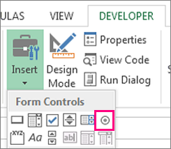
Once the box appears in the cell, copy it, highlight the cells you also want it to appear in, and then paste it.
17. Hyperlink a cell to a website.
If you’re using your sheet to track social media or website metrics, it can be helpful to have a reference column with the links each row is tracking. If you add a URL directly into Excel, it should automatically be clickable. But, if you have to hyperlink words, such as a page title or the headline of a post you’re tracking, here’s how.
Highlight the words you want to hyperlink, then press Shift K. From there a box will pop up allowing you to place the hyperlink URL. Copy and paste the URL into this box and hit or click Enter.
If the key shortcut isn’t working for any reason, you can also do this manually by highlighting the cell and clicking Insert > Hyperlink.
18. Add drop-down menus.
Sometimes, you’ll be using your spreadsheet to track processes or other qualitative things. Rather than writing words into your sheet repetitively, such as «Yes», «No», «Customer Stage», «Sales Lead», or «Prospect», you can use dropdown menus to quickly mark descriptive things about your contacts or whatever you’re tracking.
Here’s how to add drop-downs to your cells.
Highlight the cells you want the drop-downs to be in, then click the Data menu in the top navigation and press Validation.
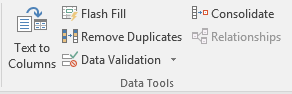
From there, you’ll see a Data Validation Settings box open. Look at the Allow options, then click Lists and select Drop-down List. Check the In-Cell dropdown button, then press OK.
19. Use the format painter.
As you’ve probably noticed, Excel has a lot of features to make crunching numbers and analyzing your data quick and easy. But if you ever spent some time formatting a sheet to your liking, you know it can get a bit tedious.
Don’t waste time repeating the same formatting commands over and over again. Use the format painter to easily copy the formatting from one area of the worksheet to another. To do so, choose the cell you’d like to replicate, then select the format painter option (paintbrush icon) from the top toolbar.
Excel Keyboard Shortcuts
Creating reports in Excel is time-consuming enough. How can we spend less time navigating, formatting, and selecting items in our spreadsheet? Glad you asked. There are a ton of Excel shortcuts out there, including some of our favorites listed below.
Create a New Workbook
PC: Ctrl-N | Mac: Command-N
Select Entire Row
PC: Shift-Space | Mac: Shift-Space
Select Entire Column
PC: Ctrl-Space | Mac: Control-Space
Select Rest of Column
PC: Ctrl-Shift-Down/Up | Mac: Command-Shift-Down/Up
Select Rest of Row
PC: Ctrl-Shift-Right/Left | Mac: Command-Shift-Right/Left
Add Hyperlink
PC: Ctrl-K | Mac: Command-K
Open Format Cells Window
PC: Ctrl-1 | Mac: Command-1
Autosum Selected Cells
PC: Alt-= | Mac: Command-Shift-T
Other Excel Help Resources
- How to Make a Chart or Graph in Excel [With Video Tutorial]
- Design Tips to Create Beautiful Excel Charts and Graphs
- Totally Free Microsoft Excel Templates That Make Marketing Easier
- How to Learn Excel Online: Free and Paid Resources for Excel Training
Use Excel to Automate Processes in Your Team
Even if you’re not an accountant, you can still use Excel to automate tasks and processes in your team. With the tips and tricks we shared in this post, you’ll be sure to use Excel to its fullest extent and get the most out of the software to grow your business.
Editor’s Note: This post was originally published in August 2017 but has been updated for comprehensiveness.

To All the Lazy r/Excel Users: What can do you do in Excel that saves you a lot of time, but that you would never tell your boss about?
I saw an AskReddit post the other day about scenarios of «This is how it’s always been done» and I got thinking about this sub.
I use excel a lot in my day to day role but the rest of my colleagues save for a few have very little knowledge of some of the more potent capabilities of the program. I started to wonder what you guys can do in excel or what templates you might have made for yourselves that you use to make an otherwise 1hr task (for someone else) into a 10minute or less job.
Would love to know!
(sorry to the mods if this type of post is not allowed!)
Содержание
- IF function
- Simple IF examples
- Common problems
- Need more help?
- Оператор If. Then. Else
- Синтаксис
- Замечания
- Пример
- См. также
- Поддержка и обратная связь
- Использование операторов If. Then. Else
- Выполнение операторов, если условие равно True
- Выполнение определенных операторов, если условие равно True, и выполнение других операторов, если оно равно False
- Проверка второго условия, если первое условие равно False
- См. также
- Поддержка и обратная связь
- If Then Else Statement in Excel VBA (explained with examples)
- Syntax – IF Then Else
- Examples of Using IF Then Statement in VBA
- Nested IF Then (Multiple IF Then statements)
- Multiple IF Then Statements
- IF Then Else Statement
- IF Then ElseIf Else Statement
- Using AND and OR in IF Then Else
- Using Not Equal to in If Then
- Using If Then Else with Loops in VBA
- Example 1 – Save and Close All Workbooks Except The Active Workbook
- Example 2 – Highlight Cells with Negative Values
- Example 3 – Hide All the Worksheet Except the Current Worksheet
- Example 4 – Extract the Numeric Part from an Alphanumeric String
- Where to Put the VBA Code?
IF function
The IF function is one of the most popular functions in Excel, and it allows you to make logical comparisons between a value and what you expect.
So an IF statement can have two results. The first result is if your comparison is True, the second if your comparison is False.
For example, =IF(C2=”Yes”,1,2) says IF(C2 = Yes, then return a 1, otherwise return a 2).

Use the IF function, one of the logical functions, to return one value if a condition is true and another value if it’s false.
IF(logical_test, value_if_true, [value_if_false])
The condition you want to test.
The value that you want returned if the result of logical_test is TRUE.
The value that you want returned if the result of logical_test is FALSE.
Simple IF examples

In the above example, cell D2 says: IF(C2 = Yes, then return a 1, otherwise return a 2)

In this example, the formula in cell D2 says: IF(C2 = 1, then return Yes, otherwise return No)As you see, the IF function can be used to evaluate both text and values. It can also be used to evaluate errors. You are not limited to only checking if one thing is equal to another and returning a single result, you can also use mathematical operators and perform additional calculations depending on your criteria. You can also nest multiple IF functions together in order to perform multiple comparisons.
 B2,”Over Budget”,”Within Budget”)» loading=»lazy»>
=IF(C2>B2,”Over Budget”,”Within Budget”)
In the above example, the IF function in D2 is saying IF(C2 Is Greater Than B2, then return “Over Budget”, otherwise return “Within Budget”)
 B2,C2-B2,»»)» loading=»lazy»>
In the above illustration, instead of returning a text result, we are going to return a mathematical calculation. So the formula in E2 is saying IF(Actual is Greater than Budgeted, then Subtract the Budgeted amount from the Actual amount, otherwise return nothing).

In this example, the formula in F7 is saying IF(E7 = “Yes”, then calculate the Total Amount in F5 * 8.25%, otherwise no Sales Tax is due so return 0)
Note: If you are going to use text in formulas, you need to wrap the text in quotes (e.g. “Text”). The only exception to that is using TRUE or FALSE, which Excel automatically understands.
Common problems
What went wrong
There was no argument for either value_if_true or value_if_False arguments. To see the right value returned, add argument text to the two arguments, or add TRUE or FALSE to the argument.
This usually means that the formula is misspelled.
Need more help?
You can always ask an expert in the Excel Tech Community or get support in the Answers community.
Источник
Оператор If. Then. Else
Выполняет один или группу операторов в зависимости от значения выражения.
Синтаксис
IfconditionThen [ statements ] [ Elseelsestatements ]
Также можно использовать синтаксис вложенных операторов:
ЕслиусловиеТогда
[ операторы ]
[ ElseIfcondition-nThen
[ elseifstatements ]]
[ Else
[ elsestatements ]]
End If
Если. Затем. Синтаксис инструкции Else содержит эти части.
| Part | Описание |
|---|---|
| Состояние | Обязательно. Одно или оба таких выражения:
Числовое выражение или строковое выражение, оцененное как True либо False. Если условие имеет значение Null, условие обрабатывается как False. Выражение формы TypeOfobjectnameIsobjecttype. Objectname — это любая ссылка на объект, а objecttype — любой допустимый тип объекта. Выражение имеет значение True, если objectname относится к типу объекта, заданному типом objecttype; В противном случае имеет значение False. |
| Операторы | Необязательный элемент в форме блока; является обязательным при использовании однострочного оператора без предложения Else. Операторы разделяются двоеточием; выполняется, если значение condition имеет значение True. |
| condition-n | Необязательный параметр. То же самое, что и condition. |
| elseifstatements | Необязательный параметр. Один или несколько операторов, которые выполняются, если соответствующее им значение condition-n равняется True. |
| elsestatements | Необязательный параметр. Один или несколько операторов, которые выполняются, если значения ни выражения condition, ни выражения condition-n не равняются True. |
Замечания
Используйте однострочный формат (первый синтаксис) для коротких простых тестов. Однако форма блока (второй синтаксис) является более функциональной и простой для чтения, выполнения и отладки.
При использовании однострочной формы возможно выполнение нескольких операторов при соответствующем условии If. Then. Все операторы должны находиться в одной строке и разделяться двоеточием:
Оператор If блочной формы должен быть первым оператором в строке. У Else, ElseIf и End If может быть номер строки или метка строки, предшествующие им в строке. Блок If должен заканчиваться оператором End If.
Чтобы определить, является ли оператор блоком If, проверьте, что следует за ключевым словом Then . Если ничего, кроме комментария, не стоит после Then на той же строке, это однострочный оператор If.
Части Else и ElseIf являются необязательными. Можно использовать сколько угодно частей ElseIf в блоке If, но они не должны стоять после Else. Блоки оператора If могут быть вложенными, то есть содержать внутри другие.
При выполнении блока If (второй синтаксис) проверяется значение condition. Еслиcondition является True, тогда выполняются операторы, стоящие после Then. Если condition равняется False, каждое условие ElseIf (если такое имеется) оценивается по порядку. При обнаружении условия со значением True выполняются операторы, следующие за относящейся к ним части Then. Если ни одно из значений, следующих за ElseIf, не равняется True (или если отсутствует ElseIf), выполняются операторы, следующие за Else. После выполнения операторов, следующих за Then либоElse, выполняются операторы после End If.
Выбор варианта Case может оказаться более полезным при оценке одного выражения с несколькими возможными действиями. Однако предложение TypeOfobjectnameIsobjecttype нельзя использовать с инструкцией Select Case .
TypeOf невозможно использовать с такими типами данных, как Long, Integer ( кроме Object).
Пример
В этом примере показаны как блочная форма оператора If. Then. Else, так и его однострочное написание. В нем также показано использование оператора If TypeOf. Then. Else.
Используйте конструкцию If TypeOf , чтобы определить, является ли элемент управления, переданный в процедуру, текстовым полем.
См. также
Поддержка и обратная связь
Есть вопросы или отзывы, касающиеся Office VBA или этой статьи? Руководство по другим способам получения поддержки и отправки отзывов см. в статье Поддержка Office VBA и обратная связь.
Источник
Использование операторов If. Then. Else
Используйте оператор If. Then. Else для выполнения определенного оператора или блока операторов в зависимости от значения условия. Операторы If. Then. Else могут быть вложены в любое необходимое число слоев.
Однако для удобства читаемости лучше использовать оператор Select Case вместо нескольких уровней вложенных операторов If. Then. Else.
Выполнение операторов, если условие равно True
Чтобы выполнить только один оператор, когда условие равно True, используйте однострочный синтаксис оператора If. Then. Else. В следующем примере показан однострочный синтаксис с ключевым словомElse.
Чтобы выполнить несколько строк кода, необходимо использовать многострочный синтаксис. Этот синтаксис включает оператор End If, как показано в примере ниже.
Выполнение определенных операторов, если условие равно True, и выполнение других операторов, если оно равно False
Используйте оператор If. Then. Else для определения двух блоков исполняемых операторов: один блок выполняется, если условие равно True, а другой блок выполняется, если условие равно False.
Проверка второго условия, если первое условие равно False
Можно добавить операторы ElseIf в оператор If. Then. Else для проверки второго условия, если первое условие равно False. Например, в следующей процедуре функция вычисляет бонус на основе классификации задания. Оператор, следующий за оператором Else, выполняется в том случае, если условия во всех операторах If и ElseIf равны False.
См. также
Поддержка и обратная связь
Есть вопросы или отзывы, касающиеся Office VBA или этой статьи? Руководство по другим способам получения поддержки и отправки отзывов см. в статье Поддержка Office VBA и обратная связь.
Источник
If Then Else Statement in Excel VBA (explained with examples)
In Excel VBA, IF Then Else statement allows you to check for a condition, and perform an action accordingly.
This is extremely valuable in many situations as we will see in the examples later in this tutorial.
To give you a simple example, suppose you have a list of grades in Excel and you want to highlight all those students who have scored an A. Now, if I ask you to do this manually, you will check each student’s grade and if it’s an A, you’ll highlight it, and if it isn’t, then you’ll leave it as is.
The same logic can be built in VBA using the If Then Else statement as well (and of course do a lot more than just highlighting grades).
In this tutorial, I’ll show you different ways the ‘If Then Else’ construct can be used in Excel VBA, and some practical examples in action.
But before I get into the specifics, let me give you the syntax of the ‘IF Then Else’ statement.
If you’re interested in learning VBA the easy way, check out my Online Excel VBA Training.
This Tutorial Covers:
Syntax – IF Then Else
Below is the generic syntax of If Then Else construct in VBA
Note that the Else part of this statement is optional.
Now if you’re wondering what’s the difference between the two syntaxes, let me clarify.
The first syntax is a simple one-line IF THEN ELSE statement where you don’t need to use the END IF statement.
However, in the second syntax, the true_code part is in the second line. This is helpful when the code that you need to run in case the IF condition is true is long and consists of multiple lines.
When you split the IF statement into multiple lines, you need to tell VBA where the IF Then construct ends.
Hence you need to use the End IF statement.
In case you don’t use End IF when required, VBA will show you an error – “Block IF without END IF”
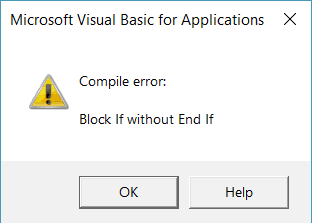
Examples of Using IF Then Statement in VBA
To give you an idea of how the IF-THEN statement works in VBA, let me start with some basic examples (some practical and more useful examples are covered later in this tutorial).
Suppose you have a student’s score in cell A1 and you want to check whether the student passed the exam or not (passing marks threshold being 35).
Then you can use the following code:
The above code has a single line of IF statement that checks the value in cell A1.
If it’s more than 35, it shows the message – “Pass”.
If it’s less than 35, nothing happens.
But what if you want to show a message in both the cases, whether a student passed or failed the exam.
The below code would do this:
The above code uses the IF as well as the ELSE statement to execute two different conditions. When the score is more than (or equal to) 35, the IF condition is true, and the code right below it gets executed (everything before the Else statement).
But when the IF condition is FALSE, the code jumps to the Else part and executes the code block in it.
Note that when we use a single line of IF Then statement, we don’t need to use End IF. But when we split it into more than one line, we need to use the End If statement.
Nested IF Then (Multiple IF Then statements)
So far we have used a single IF Then statement.
In case you have multiple conditions to check, you can use:
- Multiple IF conditions
- If Then Else statement
- IF Then ElseIf Else construct
Let me show you how these differ and how to use this in Excel VBA.
Multiple IF Then Statements
Let’s take the same example of using a student’s score.
If the student scores less than 35, the message to display is ‘Fail’, if the score is more than or equal to 35, the message to display is ‘Pass’.
We can use the below code to get this done:
You can use multiple IF Then statement as shown above. While this works, it’s not an example of good coding (as you will see the alternatives below).
In case you decide to use this, remember that these statements should either be independent or mutually exclusive. The important thing to know here is that in the above construct, all the IF statements are evaluated and the ones where the condition is true, the code is executed.
So even if the first IF statement is correct, the second would still be evaluated.
IF Then Else Statement
Suppose this time, instead of just displaying the message Pass/Fail, we have one more condition.
If the student scores less than 35, the message to display is ‘Fail’, if the score is more than or equal to 35, the message to display is ‘Pass’, and if the score is more than 80, the message to display is ‘Pass, with Distinction’.
We can use the below code to get this done:
In the above code, we have used multiple IF statements (nested IF Then) with the help of Else.
So there is an ‘IF Then Else’ construct within an ‘IF Then Else’ construct. This type of nesting allows you to check for multiple conditions and run the relevant block of code.
IF Then ElseIf Else Statement
The above code (that we saw in the previous section) can be further optimized by using the ElseIf statement.
Here is what we’re trying to do – If the student scores less than 35, the message to display is ‘Fail’, if the score is more than or equal to 35, the message to display is ‘Pass’, and if the score is more than 80, the message to display is ‘Pass, with Distinction’.
The above code uses ElseIf, which allows us to keep all the conditions within one single IF Then statement.
Using AND and OR in IF Then Else
So far in this tutorial, we have only checked for a single condition at a time.
However, when you have multiple dependent conditions, you can use the AND or OR statement with the IF conditions.
Below is the syntax of using AND/OR condition with the IF Then statement.
In the above code, only when both Condition1 and Condition2 are met, the true_code is executed. Even if one of the conditions is false, it will execute the false_code.
With OR, even if one of the conditions are true, it will execute the true_code. Only when all the conditions are false, it executes the false_code.
Now let’s see how AND and OR statement work with the IF Then Else construct.
Suppose you have the scores for two subjects instead of one, and you want to check for the following conditions:
- Fail – When the score is less than 35 in any of the subjects.
- Pass – When the score is more than or equal to 35, but less than 80 in both the subjects.
- Pass, with Distinction – When the score is more than 35 in both the subjects and is more than or equal to 80 in one or both the subjects.
Here is the code that will do this:
The above code uses both OR and AND statements.
You can also write this same code with a slight change (using OR instead of AND).
Both the above VBA codes will give you the same result. Personally, I prefer the first one as it has a logical flow of checking the scores (but that’s just me).
Using Not Equal to in If Then
In all the examples above, we have used the conditions that check whether a value equal to a specified value or not.
You can also use similar codes when checking when the value is not equal to a specified value in the VBA code. Not equal to represented by <> the Excel VBA.
To see a practical example of using <>, have a look at Example 1 below.
Using If Then Else with Loops in VBA
So far, we have been going through some examples that are good to understand how the ‘IF-THEN’ statements work in VBA, however, are not useful in the practical world.
If I need to grade students, I can easily do that using Excel functions.
So let’s have a look at some useful and practical examples that can help you automate some stuff and be more efficient.
Example 1 – Save and Close All Workbooks Except The Active Workbook
If you have a lot of workbooks open and you quickly want to close all, except the active workbook, you can use the below code,
The above code would save and close all the workbooks (except the active one).
It uses the For Next loop to go through the collection of all the open workbooks and checks the name using the IF condition.
If the name is not the same as that of the Active workbook, it saves and closes it.
In case there is a VBA code in any of the workbooks and you haven’t saved it as .xls or .xlsm, you will see a warning (as the vba codes are lost when you save it in .xlsx format).
Example 2 – Highlight Cells with Negative Values
Suppose that you have a column full of numbers and you want to quickly highlight all the cells with negative values in red, you can do that using the below code.
The above code uses the For Each loop and checks each cell in the selection that you have made. If the cell has a value that is negative, it’s highlighted in red with white font color.
Example 3 – Hide All the Worksheet Except the Current Worksheet
In case you want to quickly hide all the worksheets except the active one, you can use the below code:
The above code uses the For Each loop to go through a collection of worksheets. It checks the name of each worksheet and hides it if it’s not the active worksheet.
If you have alphanumeric strings in cells and you want to extract the numeric part from it, you can do that using the below code:
This code will create a custom function in Excel that can use within the worksheet (just like a regular function).
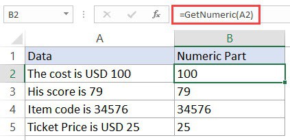
Where to Put the VBA Code?
Wondering where the VBA code goes in your Excel workbook?
Excel has a VBA backend called the VB editor. You need to copy and paste the code in the VB Editor module code window.
Here are the steps to do this:
- Go to the Developer tab.

- Click on Visual Basic option. This will open the VB editor in the backend.
- In the Project Explorer pane in the VB Editor, right-click on any object for the workbook in which you want to insert the code. If you don’t see the Project Explorer go to the View tab and click on Project Explorer.
- Go to Insert and click on Module. This will insert a module object for your workbook.
- Copy and paste the code in the module window.
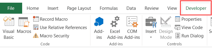
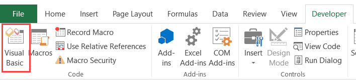
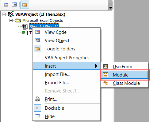
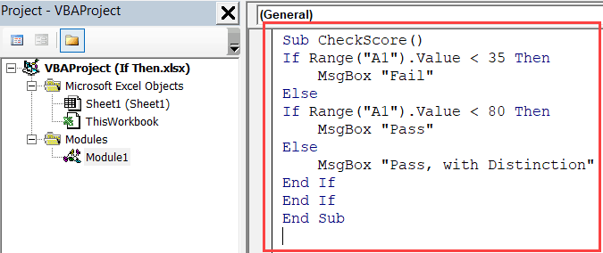
You May Also Like the Following Excel Tutorials:
Источник