What does the mean in microsoft excel - Word и Excel - помощь в работе с программами

I’m learning how to use Excel by fire. I have been given a spreadsheet. In that spreadsheet is a formula that looks like this:

=(($J$1 + $L$2)*$D$5

I’m not familiar with that syntax. Is that the same as:

=(($J1 + $L2)*$D5

I understand that $[Letter][Number] references a cell. However, I haven’t seen the syntax that uses two dollar signs $[Letter]$[Number]. What does that mean?

CharlieRB

22.5k5 gold badges55 silver badges104 bronze badges

asked Dec 16, 2015 at 19:23

Those are absolute references, they never change.

You can make it so the column never changes $C or the row never changes $2 or both never change $C$2.

This is useful when you have a constant you want to apply to a bunch of formulas that refer to something else — you can drag it down and the absolute reference won’t «walk» out of range. see —

answered Dec 16, 2015 at 19:24

RaystafarianRaystafarian

21.5k11 gold badges60 silver badges90 bronze badges

Источник

Finding the mean comes in handy when processing and analyzing all kinds of data. With Microsoft Excel’s AVERAGE function, you can quickly and easily find the mean for your values. We’ll show you how to use the function in your spreadsheets.

How Microsoft Excel Calculates the Mean

By definition, the mean for a data set is the sum of all the values in the set divided by the count of those values.

For example, if your data set contains 1, 2, 3, 4, and 5, the mean for this data set is 3. You can find it with the following formula.

(1+2+3+4+5)/5

You could type out formulas like that yourself, but Excel’s AVERAGE function helps you perform this calculation with ease.

Find the Mean Using a Function in Microsoft Excel

In our example, we’ll find the mean for the values in the “Score” column, and display the answer in the C9 cell.

We’ll start by clicking the C9 cell where we want to display the resulting mean.

In the C9 cell, we’ll type the following function. This function finds the mean for the values in all the cells between C2 and C6 (both these cells included).

=AVERAGE(C2:C6)

Press Enter and the result will appear in the C9 cell.

You can use the AVERAGE function to find the mean for any values in your spreadsheet. Enjoy!

Getting the mean will come in handy if you ever need Excel to calculate uncertainty.

RELATED: How to Get Microsoft Excel to Calculate Uncertainty

What Do the Symbols (&,$,<, etc.) Mean in Formulas? – Excel & Google Sheets

This tutorial explains what different symbols mean in formulas in Excel and Google Sheets.

Excel is essentially used for keeping track of data and using calculations to manipulate this data. All calculations in Excel are done by means of formulas, and all formulas are made up of different symbols or operators, depending on what function the formula is performing.

Equal Sign (=)

The most commonly used symbol in Excel is the equal (=) sign. Every single formula or function used has to start with equals to let Excel know that a formula is being used. If you wish to reference a cell in a formula, it has to have an equal sign before the cell address. Otherwise, Excel just shows the cell address as standard text.

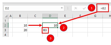
In the above example, if you type (1) =B2 in cell D2, it returns a value of (2) 10. However, typing only (3) B3 into cell D3 just shows “B3” in the cell, and there is no reference to the value 20.

Standard Operators

The next most common symbols in Excel are the standard operators as used on a calculator: plus (+), minus (–), multiply (*) and divide (/). Note that the multiplication sign is not the standard multiplication sign (x) but is depicted by an asterisk (*) while the division sign is not the standard division sign (÷) but is depicted by the forward slash (/).

An example of a formula using addition and multiplication is shown below:

Order of Operations and Adding Parentheses

In the formula shown above, B2*B3 is calculated first, as in standard mathematics. The order of operations is always multiplication before addition. However, you can adjust the order of operations by adding parentheses (round brackets) to the formula; any calculations between these parentheses would then be done first before the multiplication. Parentheses, therefore, are another example of symbols used in Excel.

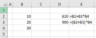
In the example shown above, the first formula returns a value of 610 while the second formula (using parentheses) returns 900.

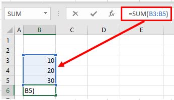
Parentheses are also used with all Excel functions. For example, to sum B3, B4, and B5 together, you can use the SUM Function where the range B3:B5 is contained within parentheses.

Colon (:) to Specify a Range of Cells

In the formula used above, the parentheses contain the cell range which the SUM Function needs to add together. This cell range is expressed with a colon (:) where the first cell reference (B3) is the cell address of the first cell included in the range of cells to add together, while the second cell reference (B5) is the cell address of the last cell included in the range.

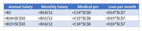
Dollar Symbol ($) in an Absolute Reference

A particular useful and common symbol used in Excel is the dollar sign within a formula. Note that this does not indicate currency; rather, it’s used to “fix” a cell address in place in order that a single cell can be used repetitively in multiple formulas by copying formulas between cells.

By adding a dollar sign ($) in front of the column header (C) and the row header (3), when copying the formula down to Rows 7–15 in the example below, the first part of the formula (e.g., C6) changes according to the row it is copied down to while the second part of the formula ($C$3) stays static always enabling the formula to refer to the value stored in cell C3.

See: Cell References and Absolute Cell Reference Shortcut for more information on absolute references.

Exclamation Point (!) to Indicate a Sheet Name

The exclamation point (!) is critical if you want to create a formula in a sheet and include a reference to a different sheet.

Square Brackets [ ] to Refer to External Workbooks

Excel uses square brackets to show references to linked workbooks. The name of the external workbook is enclosed in square brackets, while the sheet name in that workbook appears after the brackets with an exclamation point at the end.

Comma (,)

The comma has two uses in Excel.

Refer to Multiple Ranges

If you wish to use multiple ranges in a function (e.g., the SUM Function), you can use a comma to separate the ranges.

Separate Arguments in a Function

Alternatively, some built in Excel functions have multiple arguments which are usually separated with commas. (These can also be semicolons, depending on the function syntax.)

Curly Brackets in Array Formulas

Curly brackets are used in array formulas. An array formula is created by pressing the CTRL + SHIFT + ENTER keys together when entering a formula.

Other Important Symbols

Symbol Description Example

% Percentage =B2%

^ Exponential operator =B2^B3

& Concatenation =B2&B3

> Greater than =B2>B3

= Greater than or equal to =B2>=B3

Not equal to =B2<>B3

Symbols in Formulas in Google Sheets

The symbols used in Google Sheets are identical to those used in Excel.

Источник

What does $ (dollar sign) mean in Excel Formulas?

If you have worked with Excel formulas, I am sure you have noticed that sometimes there is a $ symbol as a part of the cell references.

If you’re wondering what does the $ sign means in Excel formulas/functions, this article is the right place.

Table of Contents

What does $ mean in Excel formulas?

One of the things that make Excel such a powerful tool is the ability to refer to cells/ranges and use these in formulas.

And when you copy these formulas, these cell references can adjust automatically (or should I say automatically).

Below is an example where I copy the cell C2 (which has a formula) and paste it in C3.

You can see that the formula adjusts the references when I copy and paste it. While in the formula in cell C2 refers to A2 and B2, the one in C3 refers to A3 and B3.

This is called relative reference where the references adjust based on the cell in which it has been applied.

But what if you don’t want some cells to adjust the reference?

What if you want to copy the formula, but don’t want the cell reference to change?

…. introducing the $ sign.

When you use a $ sign before the cell reference (such as $C$2), you’re telling Excel to keep referring to cell C3 even when you copy and paste the formula.

Now you can use the dollar ($) sign in three different ways, which means that there are three types of references on Excel.

Shortcut to add $ Sign to Cell References

There are two ways you can add the $ sign to a cell reference in Excel.

You can either do it manually (i.e., go into the edit mode in a cell by double-clicking on it or using F2, placing the cursor where you want the $ sign and then typing it manually).

Or you can use the keyboard shortcut

To use this shortcut, simply place the cursor on the cell reference where you want to add the dollar sign and press is once. You will notice that it will change the reference by adding/removing the $ sign (based on what’s the original reference).

For example, suppose you have the reference C2 in a cell. Here is how the F4 shortcut would work:

Press F4 one time – C2 will change to $C$2

Press F4 two times – C2 will change to C$2

Press F4 three times – C2 will change to $C2

Press F4 four times – C2 will change back to C2

Types of References in Excel

There are three types of references in Excel:

Relative references

Absolute references

Mixed references

In relative references, you don’t use a dollar ($) sign in the references at all.

In mixed references, you use the dollar sign ($) only once (such as $C3 or C$3)

In absolute reference, you use the dollar sign in twice in a reference (such as $C$3).

Let me quickly explain each of these with a simple example.

Relative reference

Relative reference is where you don’t use a dollar ($) sign at all.

And when you copy a cell that has a relative reference, it will change and adjust based on the cell where you copy it.

Below is the same example again, where the references adjust as soon as we copy and paste the cell that has the formula.

Absolute reference

In absolute references, you have the $ sign before the row number and the column alphabet (example $C$3)

When you use this in formulas, it will not change the reference

when you copy and paste the cell. This could be useful when you have some value that needs to remain constant (such as time period or interest rates, etc.)

Below is an example where I have a value in cell D2 which needs to remain constant (and not change when we copy-paste the formulas).

By using $D$2, we make sure that it doesn’t change when we copy-paste the cell with the formula.

Note that this example has both, relative cell reference (without the $ sign) and an absolute cell reference (with two $ signs).

Mixed reference

These are a little more complicated than the rest two.

In mixed cell references, you will have only one dollar sign (for example – $C3 or C$3)

When you add a dollar sign in front of the column alphabet (C in this example), it locks the column only. This means that if you copy-paste the formula that uses $C3, the column would not change, but the row can change.

And when you add a dollar sign in front of the row number (3 in this example), it locks the column only. This means that if you copy-paste the formula that uses C$3, the row would not change, but the column can change.

Here is a good article that goes in-depth about the mixed cell references in Excel.

Summary

A dollar sign means that the part of the cell reference before which it has been used is anchored or fixed.

Below is a quick summary of what $ means in Excel formulas:

$A$1 – always refers to column A and row 1

$A1 – Column A is fixed and will not change, but the row is allowed to change as the formula is copied

A$1 – Row 1 is fixed and will not change, but the column is allowed to change as the formula is copied.

$A$1:$A$100 – always refers to the range A1:A100

I hope this article helps you understand what the $ sign means in Excel and how to use it.

Other Excel tutorials you may find useful:

Источник

by Svetlana Cheusheva, updated on March 20, 2023

When analyzing numerical data, you may often be looking for some way to get the «typical» value. For this purpose, you can use the so-called measures of central tendency that represent a single value identifying the central position within a data set or, more technically, the middle or center in a statistical distribution. Sometimes, they are also classified as summary statistics.

The three main measures of central tendency are Mean, Median and Mode. They all are valid measures of central location, but each gives a different indication of a typical value, and under different circumstances some measures are more appropriate to use than others.

How to calculate mean in Excel

Arithmetic mean, also referred to as average, is probably the measure you are most familiar with. The mean is calculated by adding up a group of numbers and then dividing the sum by the count of those numbers.

For example, to calculate the mean of numbers <1, 2, 2, 3, 4, 6>, you add them up, and then divide the sum by 6, which yields 3: (1+2+2+3+4+6)/6=3.

In Microsoft Excel, the mean can be calculated by using one of the following functions:

AVERAGE- returns an average of numbers.

AVERAGEA — returns an average of cells with any data (numbers, Boolean and text values).

AVERAGEIF — finds an average of numbers based on a single criterion.

AVERAGEIFS — finds an average of numbers based on multiple criteria.

For the in-depth tutorials, please follow the above links. To get a conceptual idea of how these functions work, consider the following example.

In a sales report (please see the screenshot below), supposing you want to get the average of values in cells C2:C8. For this, use this simple formula:

To get the average of only «Banana» sales, use an AVERAGEIF formula:

=AVERAGEIF(A2:A8, «Banana», C2:C8)

To calculate the mean based on 2 conditions, say, the average of «Banana» sales with the status «Delivered», use AVERAGEIFS:

=AVERAGEIFS(C2:C8,A2:A8, «Banana», B2:B8, «Delivered»)

You can also enter your conditions in separate cells, and reference those cells in your formulas, like this: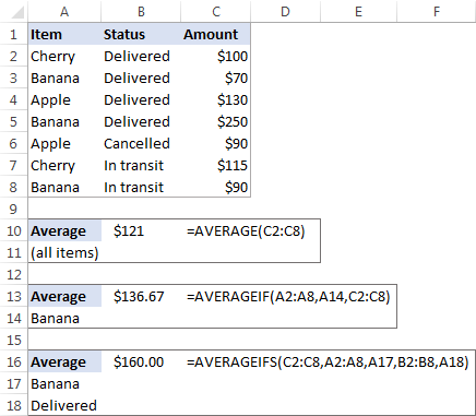

Median is the middle value in a group of numbers, which are arranged in ascending or descending order, i.e. half the numbers are greater than the median and half the numbers are less than the median. For example, the median of the data set <1, 2, 2, 3, 4, 6, 9>is 3.

This works fine when there are an odd number of values in the group. But what if you have an even number of values? In this case, the median is the arithmetic mean (average) of the two middle values. For example, the median of <1, 2, 2, 3, 4, 6>is 2.5. To calculate it, you take the 3rd and 4th values in the data set and average them to get a median of 2.5.

In Microsoft Excel, a median is calculated by using the MEDIAN function. For example, to get the median of all amounts in our sales report, use this formula:

To make the example more illustrative, I’ve sorted the numbers in column C in ascending order (though it is not actually required for the Excel Median formula to work):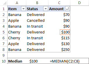

In contrast to average, Microsoft Excel does not provide any special function to calculate median with one or more conditions. However, you can «emulate» the functionality of MEDIANIF and MEDIANIFS by using a combination of two or more functions like shown in these examples:

How to calculate mode in Excel

Mode is the most frequently occurring value in the dataset. While the mean and median require some calculations, a mode value can be found simply by counting the number of times each value occurs.

For example, the mode of the set of values <1, 2, 2, 3, 4, 6>is 2. In Microsoft Excel, you can calculate a mode by using the function of the same name, the MODE function. For our sample data set, the formula goes as follows:

=MODE(C2:C8)

In situations when there are two or more modes in your data set, the Excel MODE function will return the lowest mode.

Generally, there is no «best» measure of central tendency. Which measure to use mostly depends on the type of data you are working with as well as your understanding of the «typical value» you are attempting to estimate.

For a symmetrical distribution (in which values occur at regular frequencies), the mean, median and mode are the same. For a skewed distribution (where there are a small number of extremely high or low values), the three measures of central tendency may be different.

Since the mean is greatly affected by skewed data and outliers (non-typical values that are significantly different from the rest of the data), median is the preferred measure of central tendency for an asymmetrical distribution.

For instance, it is generally accepted that the median is better than the mean for calculating a typical salary. Why? The best way to understand this would be from an example. Please have a look at a few sample salaries for common jobs:

Electrician — $20/hour

Nurse — $26/hour

Police officer — $47/hour

Sales manager — $54/hour

Manufacturing engineer — $63/hour

Now, let’s calculate the average (mean): add up the above numbers and divide by 5: (20+26+47+54+63)/5=42. So, the average wage is $42/hour. The median wage is $47/hour, and it is the police officer who earns it (1/2 wages are lower, and 1/2 are higher). Well, in this particular case the mean and median give similar numbers.

But let’s see what happens if we extend the list of wages by including a celebrity who earns, say, about $30 million/year, which is roughly $14,500/hour. Now, the average wage becomes $2,451.67/hour, a wage that no one earns! By contrast, the median is not significantly changed by this one outlier, it is $50.50/hour.

Agree, the median gives a better idea of what people typically earn because it is not so strongly affected by abnormal salaries.

This is how you calculate mean, median and mode in Excel. I thank you for reading and hope to see you on our blog next week!

Источник

Источник

This tutorial explains what different symbols mean in formulas in Excel and Google Sheets.

Equal Sign (=)

Standard Operators

An example of a formula using addition and multiplication is shown below:

=B1+B2*B3

Order of Operations and Adding Parentheses

=(B1+B2)*B3

In the example shown above, the first formula returns a value of 610 while the second formula (using parentheses) returns 900.

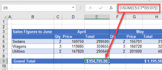
Parentheses are also used with all Excel functions. For example, to sum B3, B4, and B5 together, you can use the SUM Function where the range B3:B5 is contained within parentheses.

=SUM(B3:B5)

Colon (:) to Specify a Range of Cells

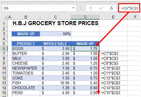
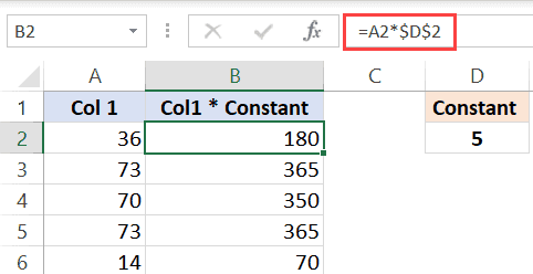
Dollar Symbol ($) in an Absolute Reference

=C6*$C$3

See: Cell References and Absolute Cell Reference Shortcut for more information on absolute references.

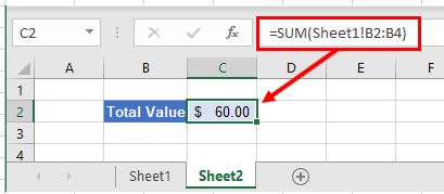
Exclamation Point (!) to Indicate a Sheet Name

The exclamation point (!) is critical if you want to create a formula in a sheet and include a reference to a different sheet.

=SUM(Sheet1!B2:B4)

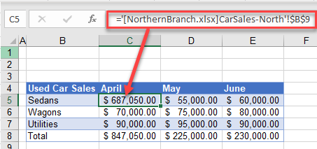
Square Brackets [ ] to Refer to External Workbooks

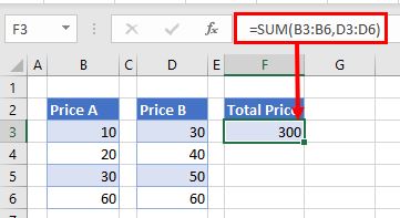
Comma (,)

The comma has two uses in Excel.

Refer to Multiple Ranges

If you wish to use multiple ranges in a function (e.g., the SUM Function), you can use a comma to separate the ranges.

=SUM(B2:B3, B6:B10)

Separate Arguments in a Function

Alternatively, some built in Excel functions have multiple arguments which are usually separated with commas. (These can also be semicolons, depending on the function syntax.)

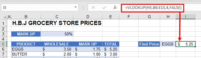
=VLOOKUP(H5, B6:E15, 4, FALSE)

Curly Brackets { } in Array Formulas

Curly brackets are used in array formulas. An array formula is created by pressing the CTRL + SHIFT + ENTER keys together when entering a formula.

Other Important Symbols

Symbol	Description	Example
%	Percentage	=B2%
^	Exponential operator	=B2^B3
&	Concatenation	=B2&B3
>	Greater than	=B2>B3
<	Less than	=B2<B3
>=	Greater than or equal to	=B2>=B3
<=	Less than or equal to	=B2<=B3
<>	Not equal to	=B2<>B3

Symbols in Formulas in Google Sheets

The symbols used in Google Sheets are identical to those used in Excel.

Источник

What Does Mean In Excel? We all have this question in our mind and when we are using Excel, then we have this question a lot of times. Because mean does a lot of things in Microsoft Excel. So here we are going to talk about the Mean in Microsoft Excel and also we will answer the question that what does mean operator in Excel.

So here without any delay let’s start knowing more about Mean and what does mean in excel. You will find that Mean means exactly the way it is meant in real life or Mathematics.

Mean is Average of Number of Values

It is very simple for all of us. Because we have studied about mean in school days, that Mean is the average. Whenever we have ‘N’ Number of values and we want to get it’s average, we call it Mean. So mean works as same as Average. In Mathematics sometimes we also use Mean and refer Mean as the middle value of some numbers.

But here we are going to tell you what does mean in Excel and what are the specified formulas that we can use to get the mean out of a lot of numbers or the values.

Mean Only Applicable To Numbers

Before going further, let us make it very clear to you that Mean is only applicable to the mathematical values. So numerical values are only used to get the mean out of them. You cant get mean of alphabets or any other special values. Only numeric values are used to find out the mean in Microsoft Excel or anywhere else.

Here is the Formula to Find the Mean

The basic formula to find out the Mean is simply to put the sum of all the values and then divide that sum with the total number of values used. Keep in mind that this formula is basic and used in mathematical statements.

But when we are going to find out Mean in Microsoft then we have to use this formula in a format that is specially made up for Microsoft Excel. So the exact meaning of What does mean in Excel will come in the next paragraph. For now, you can assume the Mean formula in the outer world as a sum of numbers divided by total numbers.

Microsoft Excel Formula to find Mean

Write down the numerical values if you want to find out the arithmetic mean of numbers. Not only you will get mean in this example but also you will get a very clear picture of what does mean in Excel. So count the number of values you have in total. Now go to an empty cell and write down the excel formula to find out the Average or Arithmetic Mean.

The formula is “=AVERAGE(A: A)” Here A means the starting cell which has value and the next A means the last cell which has a numerical value.

Now press “Enter” to get the answer. After you press the Enter you will get the right answer which will be the mean of your numbers.

You Can Also Read These:

How to Create a Calendar in Excel – Step by Step Guide
How to Turn Off Scroll Lock
What Is Absolute Cell Reference In Excel

Источник