
Содержание
- Excel help & learning
- Learn from live instructors
- Explore Excel
- Create a new workbook
- Create a workbook
- Create a workbook from a template
- Open a new, blank workbook
- Base a new workbook on an existing workbook
- Base a new workbook on a template
- Need more help?
- How to Create Documents in MS Excel
- Related
- Create Spreadsheet in Excel
- Introduction to Create Spreadsheet in Excel
- How to Create a Spreadsheet in Excel?
- Example #1 – How to Create Spreadsheet in Excel?
- Example #2 – How to Create a Simple Budget Spreadsheet in Excel?
- Example #3 – How to Create a Personal Monthly Budget Spreadsheet in Excel?
- Things to Remember
- How to add data in a spreadsheet Video
- Recommended Articles
Excel help & learning

Learn from live instructors
Microsoft offers live coaching on how to work with Excel. We’ll have you dazzling with your new skills in no time! (Available in English only.)
Explore Excel
 Find Excel templates
Bring your ideas to life and streamline your work by starting with professionally designed, fully customizable templates from Microsoft Create.
 Analyze Data
Ask questions about your data without having to write complicated formulas. Not available in all locales.
 Plan and track your health
Tackle your health and fitness goals, stay on track of your progress, and be your best self with help from Excel.
 Support for Excel 2010 has ended
Learn what end of Excel 2010 support means for you and find out how you can upgrade to Microsoft 365.
Источник
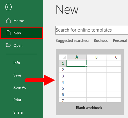
Create a new workbook
A workbook is a file that contains one or more worksheets to help you organize data. You can create a new workbook from a blank workbook or a template.

Create a workbook
Select Blank workbook or press Ctrl+N.
Create a workbook from a template
Select File > New.
Double-click a template.
Click and start typing.
Open a new, blank workbook
Click the File tab.
Under Available Templates, double-click Blank Workbook.
Keyboard shortcut To quickly create a new, blank workbook, you can also press CTRL+N.
By default, a new workbook contains three worksheets, but you can change the number of worksheets that you want a new workbook to contain.
You can also add and remove worksheets as needed.
For more information about how to add or remove worksheets, see Insert or delete a worksheet.
Base a new workbook on an existing workbook
Click the File tab.
Under Templates, click New from existing.
In the New from Existing Workbook dialog box, browse to the drive, folder, or Internet location that contains the workbook that you want to open.
Click the workbook, and then click Create New.
Base a new workbook on a template
Click the File tab.
Do one of the following:
To use one of the sample templates that come with Excel, under Available Templates, click Sample Templates and then double-click the template that you want.
To use a recently used template, click Recent Templates, and then double-click the template that you want.
To use your own template, on the My Templates, and then on the Personal Templates tab in the New dialog box, double-click the template that you want.
Note: The Personal Templates tab lists the templates that you have created. If you do not see the template that you want to use, make sure that it is located in the correct folder. Custom templates are typically stored in the Templates folder, which is usually C:Usersuser_nameAppDataLocalMicrosoftTemplates in Windows Vista, and C:Documents and Settingsuser_nameApplication DataMicrosoftTemplates in Microsoft Windows XP.
Tip: To obtain more workbook templates, you can download them from Microsoft Office.com. In Available Templates, under Office.com Templates, click a specific template category, and then double-click the template that you want to download.
Need more help?
You can always ask an expert in the Excel Tech Community or get support in the Answers community.
Источник
How to Create Documents in MS Excel

Microsoft Office Excel helps small-business owners analyze price trends, collect demographic data to improve your marketing efforts and produce customized reports for your bank or investors. The foundation of Excel is a workbook. Each Excel workbook is a separate document, within which you create one or several worksheets.
Open Excel by clicking «All Programs» in the Windows “Start” menu. Scroll through the list of programs to find the Microsoft Office folder and click to open it. Locate Microsoft Excel in this list and click on the program’s name to open the application.
Place your cursor in the column and row where you want to enter your labels or numbers. Users often leave one or two blank rows at the top of an Excel worksheet to use for notes or instructions. The intersection of a column and a row is a cell. Excel displays the location of your cursor each time you place it in a cell: Columns are identified by letters, and rows by numbers.
Create labels that help you identify the data in your worksheet. In a worksheet that contains data for an entire year, you could enter the name of each month on the same row, starting with January in column A and ending with December in column L. To type your labels in columns, place your cursor in the first row that you are using and enter text in each row of the same column.
Enter your numerical data below your row labels or beside your column labels. For Excel spreadsheets, each data cell in your worksheet can contain text, numbers or formulae.
Place your cursor in an empty cell below your last column of numbers or at the end of a row of numbers to insert formulas and calculate your numerical data. Click the “Sum” button on the Excel toolbar to select all of the cells in that row or column and add them. Press «Enter» or click the check mark in the Excel formula bar to put the formula into the worksheet.
Start a custom Excel formula by typing the equal sign on your keyboard. Click the first cell that you want in the formula with your mouse, then type the arithmetic symbols on your keyboard for multiply, divide, add or subtract. Click the next number that you need in the formula. Continue selecting cells and typing arithmetic functions until you finish the formula
Save your document. Click the «File» tab at the top of your worksheet. Choose «Save» from the menu. Type a name for your document in the dialogue box and confirm your action by clicking «Save.»
Источник
Create Spreadsheet in Excel
Create Spreadsheet in Excel (Table of Content)
Introduction to Create Spreadsheet in Excel
A spreadsheet is a grid-based file designed to manage or perform any type of calculation on personal or business data. It is accessible in both Office 365 and MS Office. Office 365 is a cloud-based application, whereas MS Office is an on-premises solution. It is the best choice for users because it has 400+ functions and features such as pivot, coloring, graph, chart, and conditional formatting.
Excel functions, formula, charts, formatting creating excel dashboard & others
The workbook is the Excel lingo for ‘spreadsheet.’ MS Excel uses this term to emphasize that a single workbook can contain multiple worksheets, each with its own data grid, chart, or graph.
How to Create a Spreadsheet in Excel?
Here are a few examples of creating different types of spreadsheets in excel with the key features of the created spreadsheets.
Example #1 – How to Create Spreadsheet in Excel?
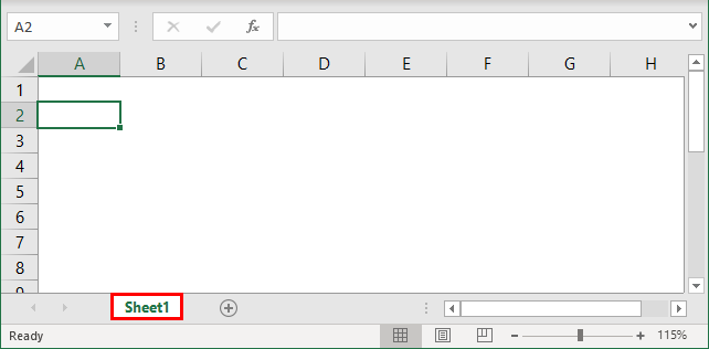
Step 1: Open MS Excel.
Step 2: Go to Menu and select New >> click on the Blank workbook to create a simple worksheet.
OR – Press Ctrl + N: To create a new spreadsheet.
Step 3: By default, Sheet1 will be created as a worksheet in the spreadsheet. The name of the spreadsheet will be given as Book1 if you are opening it for the first time.
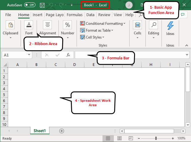
Key Features of the Created Spreadsheet:
- Basic App Functions Area: There is a green banner that contains all types of actions to perform on the worksheet, like – save the file, back or front step move, new, undo, redo, and many more.
- Ribbon Area: This is a gray area just below the basic app functions area and is called Ribbon. It contains data manipulation, a data visualizing toolbar, page layout tools, and many more.
- Spreadsheet Work Area: By default, a grid contains alphabetic columns like A, B, C, …, Z, ZA…, ZZ, ZZA… and rows as numbers like 1,2 3, …. 100, 101, and… so on. Each rectangle box in the spreadsheet is called a cell, like the one selected in the above image (cell A1). It is a cell where the user can perform their calculation for personal or business data.
- Formula Bar: It shows the data in the selected cell; if it contains any formula, it will show here. Like the above area, a search bar is available in the top right corner, and a sheet tab is available on the downside of the worksheet. A user can change the name of the sheet name.
Once you create an Excel Spreadsheet, you can convert it to a universally accepted format like PDF. For convenience, some useful Excel to PDF converters converts Excel to PDF files for free while maintaining the original formatting.
Example #2 – How to Create a Simple Budget Spreadsheet in Excel?
Let’s suppose a user wishes to design a spreadsheet for budget calculation. For the year 2018, he has a few products and their quarterly sales. He now wants to present his client with this budget.
Let’s see how we can do this with the help of the spreadsheet.
Step 1: Open MS Excel.
Step 2: Go to Menu and select New >> click on the Blank workbook to create a simple worksheet.
OR – Press Ctrl + N: To create a new spreadsheet.

Step 3: Go to the spreadsheet work area. Which is sheet1.
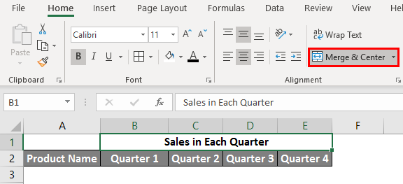
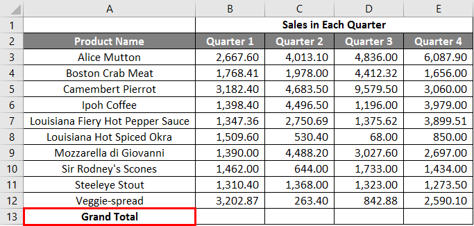
Step 4: Now create headers for Sales in each quarter in the first row by merging cells from B1 to E1. In row 2, give the product name and each quarter’s name.
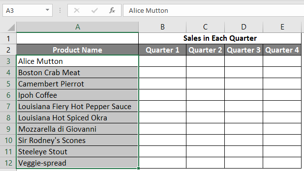
Step 5: Write down all product names in column A.
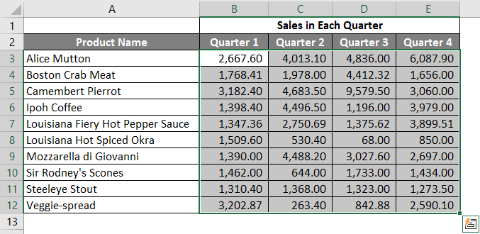
Step 6: Provide the sales data for each quarter in front of every product.
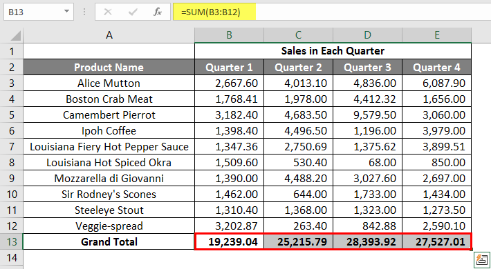
Step 7: Now, in the next row, put one header for Grand Total and calculate each quarter’s total sales.
Step 8: Calculate the grand total for each quarter by summation >> apply in other cells in B13 to E13.
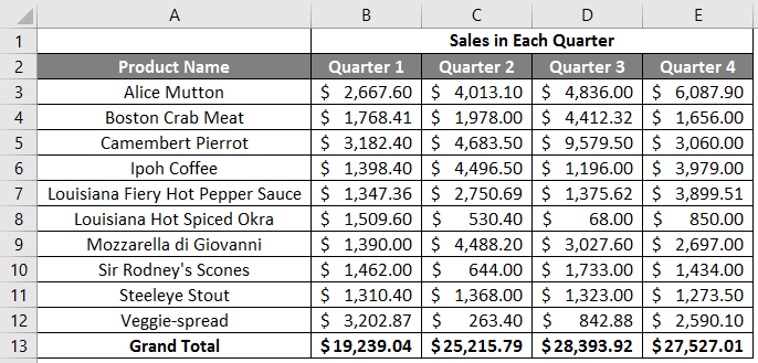
Step 9: So, let’s convert the sales value into the ($) currency symbol.
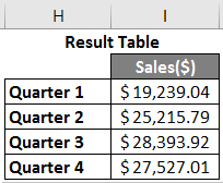
Step 10: Now, create a Result Table that has each quarter’s total sales.
Step 11: Plot the pie chart to represent the data to the client in a professional way that looks attractive. A user can change the look of the graph by just clicking on it.
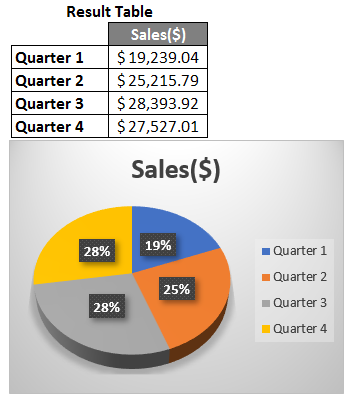
Summary of Example 2: As the user wants to create a spreadsheet to represent sales data to the client, it is done here.
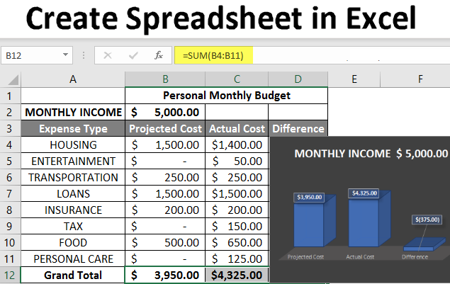
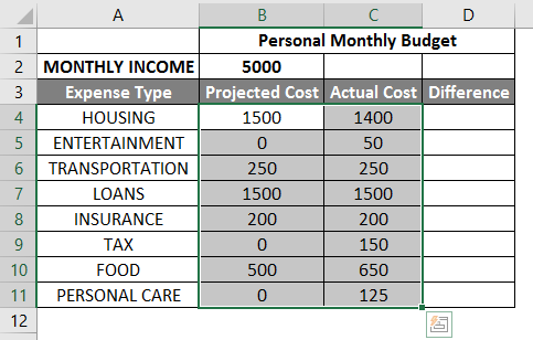
Example #3 – How to Create a Personal Monthly Budget Spreadsheet in Excel?
Let’s assume a user wants to create a spreadsheet to determine their monthly personal budget. For the year 2022, he has estimated costs and actual costs. He now wants to show his family this budget.
Let’s see how we can do this with the help of the spreadsheet.
Step 1: Open MS Excel.
Step 2: Go to Menu and select New >> click on the Blank workbook to create a simple worksheet.
OR – Press Ctrl + N: To create a new spreadsheet.

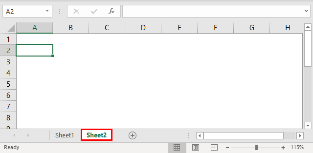
Step 3: Go to the spreadsheet work area. which is Sheet2.
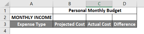
Step 4: Now create headers for Personal Monthly Budget in the first row by merging cells from B1 to D1. In row 2, give MONTHLY INCOME; in row 3, give Expense type, Projected Cost, Actual Cost, and Difference.
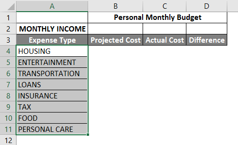
Step 5: Now, write down all the expenses in column A.
Step 6: Now, provide the monthly income, Projected cost, and Actual Cost data for each expense type.
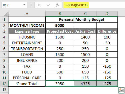
Step 7: In the next row, put one header for Grand Total and calculate the total and difference as well from the project to the actual cost.
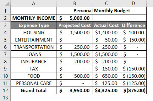
Step 8: Now highlight the header and add boundaries by using toolbar graphics. >> the cost and income value in $, so make it by currency symbol.
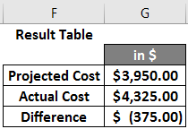
Step 9: Create a Result Table that has each quarter’s total sales.
Step 10: Plot the pie chart to represent the data for the family. A user can choose one which he likes.
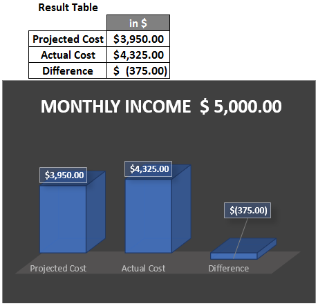
Summary of Example 3: As the user wanted to create a spreadsheet to represent monthly budget data to the family, we have created the same here. The close bracket shows in the data for the negative value.
Things to Remember
- A spreadsheet is a grid-based file designed to manage or perform any type of calculation on personal or business data.
- It is available in MS office as well as Office 365.
- The workbook is the Excel lingo for ‘spreadsheet.’ MS Excel uses this term to emphasize that a single workbook can contain multiple worksheets.
How to add data in a spreadsheet Video
Recommended Articles
This is a comprehensive guide to creating Spreadsheets in Excel. Here we have discussed how to create a Spreadsheet in Excel, examples, and a downloadable excel template. You may also look at the following articles to learn more –
Источник
Sometimes, Excel seems too good to be true. All I have to do is enter a formula, and pretty much anything I’d ever need to do manually can be done automatically.
Need to merge two sheets with similar data? Excel can do it.
Need to do simple math? Excel can do it.
Need to combine information in multiple cells? Excel can do it.
In this post, I’ll go over the best tips, tricks, and shortcuts you can use right now to take your Excel game to the next level. No advanced Excel knowledge required.
![Download 10 Excel Templates for Marketers [Free Kit]](https://no-cache.hubspot.com/cta/default/53/9ff7a4fe-5293-496c-acca-566bc6e73f42.png)
-
What is Excel?
-
Excel Basics
-
How to Use Excel
-
Excel Tips
-
Excel Keyboard Shortcuts
What is Excel?
Microsoft Excel is powerful data visualization and analysis software, which uses spreadsheets to store, organize, and track data sets with formulas and functions. Excel is used by marketers, accountants, data analysts, and other professionals. It’s part of the Microsoft Office suite of products. Alternatives include Google Sheets and Numbers.
Find more Excel alternatives here.
What is Excel used for?
Excel is used to store, analyze, and report on large amounts of data. It is often used by accounting teams for financial analysis, but can be used by any professional to manage long and unwieldy datasets. Examples of Excel applications include balance sheets, budgets, or editorial calendars.
Excel is primarily used for creating financial documents because of its strong computational powers. You’ll often find the software in accounting offices and teams because it allows accountants to automatically see sums, averages, and totals. With Excel, they can easily make sense of their business’ data.
While Excel is primarily known as an accounting tool, professionals in any field can use its features and formulas — especially marketers — because it can be used for tracking any type of data. It removes the need to spend hours and hours counting cells or copying and pasting performance numbers. Excel typically has a shortcut or quick fix that speeds up the process.
You can also download Excel templates below for all of your marketing needs.
After you download the templates, it’s time to start using the software. Let’s cover the basics first.
Excel Basics
If you’re just starting out with Excel, there are a few basic commands that we suggest you become familiar with. These are things like:
- Creating a new spreadsheet from scratch.
- Executing basic computations like adding, subtracting, multiplying, and dividing.
- Writing and formatting column text and titles.
- Using Excel’s auto-fill features.
- Adding or deleting single columns, rows, and spreadsheets. (Below, we’ll get into how to add things like multiple columns and rows.)
- Keeping column and row titles visible as you scroll past them in a spreadsheet, so that you know what data you’re filling as you move further down the document.
- Sorting your data in alphabetical order.
Let’s explore a few of these more in-depth.
For instance, why does auto-fill matter?
If you have any basic Excel knowledge, it’s likely you already know this quick trick. But to cover our bases, allow me to show you the glory of autofill. This lets you quickly fill adjacent cells with several types of data, including values, series, and formulas.
There are multiple ways to deploy this feature, but the fill handle is among the easiest. Select the cells you want to be the source, locate the fill handle in the lower-right corner of the cell, and either drag the fill handle to cover cells you want to fill or just double click:
 Similarly, sorting is an important feature you’ll want to know when organizing your data in Excel.
Sometimes you may have a list of data that has no organization whatsoever. Maybe you exported a list of your marketing contacts or blog posts. Whatever the case may be, Excel’s sort feature will help you alphabetize any list.
Click on the data in the column you want to sort. Then click on the «Data» tab in your toolbar and look for the «Sort» option on the left. If the «A» is on top of the «Z,» you can just click on that button once. If the «Z» is on top of the «A,» click on the button twice. When the «A» is on top of the «Z,» that means your list will be sorted in alphabetical order. However, when the «Z» is on top of the «A,» that means your list will be sorted in reverse alphabetical order.
Let’s explore more of the basics of Excel (along with advanced features) next.
To use Excel, you only need to input the data into the rows and columns. And then you’ll use formulas and functions to turn that data into insights.
We’re going to go over the best formulas and functions you need to know. But first, let’s take a look at the types of documents you can create using the software. That way, you have an overarching understanding of how you can use Excel in your day-to-day.
Documents You Can Create in Excel
Not sure how you can actually use Excel in your team? Here is a list of documents you can create:
- Income Statements: You can use an Excel spreadsheet to track a company’s sales activity and financial health.
- Balance Sheets: Balance sheets are among the most common types of documents you can create with Excel. It allows you to get a holistic view of a company’s financial standing.
- Calendar: You can easily create a spreadsheet monthly calendar to track events or other date-sensitive information.
Here are some documents you can create specifically for marketers.
- Marketing Budgets: Excel is a strong budget-keeping tool. You can create and track marketing budgets, as well as spend, using Excel. If you don’t want to create a document from scratch, download our marketing budget templates for free.
- Marketing Reports: If you don’t use a marketing tool such as Marketing Hub, you might find yourself in need of a dashboard with all of your reports. Excel is an excellent tool to create marketing reports. Download free Excel marketing reporting templates here.
- Editorial Calendars: You can create editorial calendars in Excel. The tab format makes it extremely easy to track your content creation efforts for custom time ranges. Download a free editorial content calendar template here.
- Traffic and Leads Calculator: Because of its strong computational powers, Excel is an excellent tool to create all sorts of calculators — including one for tracking leads and traffic. Click here to download a free premade lead goal calculator.
This is only a small sampling of the types of marketing and business documents you can create in Excel. We’ve created an extensive list of Excel templates you can use right now for marketing, invoicing, project management, budgeting, and more.
In the spirit of working more efficiently and avoiding tedious, manual work, here are a few Excel formulas and functions you’ll need to know.
Excel Formulas
It’s easy to get overwhelmed by the wide range of Excel formulas that you can use to make sense out of your data. If you’re just getting started using Excel, you can rely on the following formulas to carry out some complex functions — without adding to the complexity of your learning path.
- Equal sign: Before creating any formula, you’ll need to write an equal sign (=) in the cell where you want the result to appear.
- Addition: To add the values of two or more cells, use the + sign. Example: =C5+D3.
- Subtraction: To subtract the values of two or more cells, use the — sign. Example: =C5-D3.
- Multiplication: To multiply the values of two or more cells, use the * sign. Example: =C5*D3.
- Division: To divide the values of two or more cells, use the / sign. Example: =C5/D3.
Putting all of these together, you can create a formula that adds, subtracts, multiplies, and divides all in one cell. Example: =(C5-D3)/((A5+B6)*3).
For more complex formulas, you’ll need to use parentheses around the expressions to avoid accidentally using the PEMDAS order of operations. Keep in mind that you can use plain numbers in your formulas.
Excel Functions
Excel functions automate some of the tasks you would use in a typical formula. For instance, instead of using the + sign to add up a range of cells, you’d use the SUM function. Let’s look at a few more functions that will help automate calculations and tasks.
- SUM: The SUM function automatically adds up a range of cells or numbers. To complete a sum, you would input the starting cell and the final cell with a colon in between. Here’s what that looks like: SUM(Cell1:Cell2). Example: =SUM(C5:C30).
- AVERAGE: The AVERAGE function averages out the values of a range of cells. The syntax is the same as the SUM function: AVERAGE(Cell1:Cell2). Example: =AVERAGE(C5:C30).
- IF: The IF function allows you to return values based on a logical test. The syntax is as follows: IF(logical_test, value_if_true, [value_if_false]). Example: =IF(A2>B2,»Over Budget»,»OK»).
- VLOOKUP: The VLOOKUP function helps you search for anything on your sheet’s rows. The syntax is: VLOOKUP(lookup value, table array, column number, Approximate match (TRUE) or Exact match (FALSE)). Example: =VLOOKUP([@Attorney],tbl_Attorneys,4,FALSE).
- INDEX: The INDEX function returns a value from within a range. The syntax is as follows: INDEX(array, row_num, [column_num]).
- MATCH: The MATCH function looks for a certain item in a range of cells and returns the position of that item. It can be used in tandem with the INDEX function. The syntax is: MATCH(lookup_value, lookup_array, [match_type]).
- COUNTIF: The COUNTIF function returns the number of cells that meet a certain criteria or have a certain value. The syntax is: COUNTIF(range, criteria). Example: =COUNTIF(A2:A5,»London»).
Okay, ready to get into the nitty-gritty? Let’s get to it. (And to all the Harry Potter fans out there … you’re welcome in advance.)
Excel Tips
- Use Pivot tables to recognize and make sense of data.
- Add more than one row or column.
- Use filters to simplify your data.
- Remove duplicate data points or sets.
- Transpose rows into columns.
- Split up text information between columns.
- Use these formulas for simple calculations.
- Get the average of numbers in your cells.
- Use conditional formatting to make cells automatically change color based on data.
- Use IF Excel formula to automate certain Excel functions.
- Use dollar signs to keep one cell’s formula the same regardless of where it moves.
- Use the VLOOKUP function to pull data from one area of a sheet to another.
- Use INDEX and MATCH formulas to pull data from horizontal columns.
- Use the COUNTIF function to make Excel count words or numbers in any range of cells.
- Combine cells using ampersand.
- Add checkboxes.
- Hyperlink a cell to a website.
- Add drop-down menus.
- Use the format painter.
Note: The GIFs and visuals are from a previous version of Excel. When applicable, the copy has been updated to provide instruction for users of both newer and older Excel versions.
1. Use Pivot tables to recognize and make sense of data.
Pivot tables are used to reorganize data in a spreadsheet. They won’t change the data that you have, but they can sum up values and compare different information in your spreadsheet, depending on what you’d like them to do.
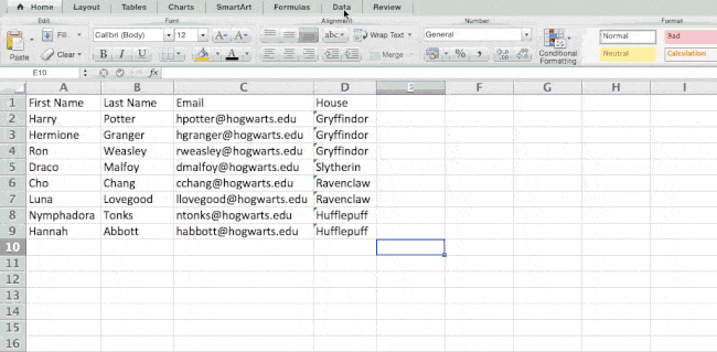
Let’s take a look at an example. Let’s say I want to take a look at how many people are in each house at Hogwarts. You may be thinking that I don’t have too much data, but for longer data sets, this will come in handy.
To create the Pivot Table, I go to Data > Pivot Table. If you’re using the most recent version of Excel, you’d go to Insert > Pivot Table. Excel will automatically populate your Pivot Table, but you can always change around the order of the data. Then, you have four options to choose from.
- Report Filter: This allows you to only look at certain rows in your dataset. For example, if I wanted to create a filter by house, I could choose to only include students in Gryffindor instead of all students.
- Column Labels: These would be your headers in the dataset.
- Row Labels: These could be your rows in the dataset. Both Row and Column labels can contain data from your columns (e.g. First Name can be dragged to either the Row or Column label — it just depends on how you want to see the data.)
- Value: This section allows you to look at your data differently. Instead of just pulling in any numeric value, you can sum, count, average, max, min, count numbers, or do a few other manipulations with your data. In fact, by default, when you drag a field to Value, it always does a count.
Since I want to count the number of students in each house, I’ll go to the Pivot table builder and drag the House column to both the Row Labels and the Values. This will sum up the number of students associated with each house.
2. Add more than one row or column.
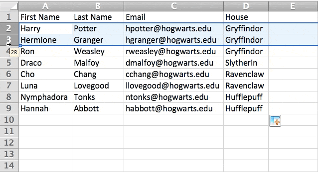
As you play around with your data, you might find you’re constantly needing to add more rows and columns. Sometimes, you may even need to add hundreds of rows. Doing this one-by-one would be super tedious. Luckily, there’s always an easier way.
To add multiple rows or columns in a spreadsheet, highlight the same number of preexisting rows or columns that you want to add. Then, right-click and select «Insert.»
In the example below, I want to add an additional three rows. By highlighting three rows and then clicking insert, I’m able to add an additional three blank rows into my spreadsheet quickly and easily.
3. Use filters to simplify your data.
When you’re looking at very large data sets, you don’t usually need to be looking at every single row at the same time. Sometimes, you only want to look at data that fit into certain criteria.
That’s where filters come in.
Filters allow you to pare down your data to only look at certain rows at one time. In Excel, a filter can be added to each column in your data — and from there, you can then choose which cells you want to view at once.
Let’s take a look at the example below. Add a filter by clicking the Data tab and selecting «Filter.» Clicking the arrow next to the column headers and you’ll be able to choose whether you want your data to be organized in ascending or descending order, as well as which specific rows you want to show.
In my Harry Potter example, let’s say I only want to see the students in Gryffindor. By selecting the Gryffindor filter, the other rows disappear.
 Pro Tip: Copy and paste the values in the spreadsheet when a Filter is on to do additional analysis in another spreadsheet.
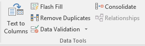
4. Remove duplicate data points or sets.
Larger data sets tend to have duplicate content. You may have a list of multiple contacts in a company and only want to see the number of companies you have. In situations like this, removing the duplicates comes in quite handy.
To remove your duplicates, highlight the row or column that you want to remove duplicates of. Then, go to the Data tab and select «Remove Duplicates» (which is under the Tools subheader in the older version of Excel). A pop-up will appear to confirm which data you want to work with. Select «Remove Duplicates,» and you’re good to go.
You can also use this feature to remove an entire row based on a duplicate column value. So if you have three rows with Harry Potter’s information and you only need to see one, then you can select the whole dataset and then remove duplicates based on email. Your resulting list will have only unique names without any duplicates.
5. Transpose rows into columns.
When you have rows of data in your spreadsheet, you might decide you actually want to transform the items in one of those rows into columns (or vice versa). It would take a lot of time to copy and paste each individual header — but what the transpose feature allows you to do is simply move your row data into columns, or the other way around.
Start by highlighting the column that you want to transpose into rows. Right-click it, and then select «Copy.» Next, select the cells on your spreadsheet where you want your first row or column to begin. Right-click on the cell, and then select «Paste Special.» A module will appear — at the bottom, you’ll see an option to transpose. Check that box and select OK. Your column will now be transferred to a row or vice-versa.
On newer versions of Excel, a drop-down will appear instead of a pop-up.

6. Split up text information between columns.
What if you want to split out information that’s in one cell into two different cells? For example, maybe you want to pull out someone’s company name through their email address. Or perhaps you want to separate someone’s full name into a first and last name for your email marketing templates.
Thanks to Excel, both are possible. First, highlight the column that you want to split up. Next, go to the Data tab and select «Text to Columns.» A module will appear with additional information.
First, you need to select either «Delimited» or «Fixed Width.»
- «Delimited» means you want to break up the column based on characters such as commas, spaces, or tabs.
- «Fixed Width» means you want to select the exact location on all the columns that you want the split to occur.
In the example case below, let’s select «Delimited» so we can separate the full name into first name and last name.
Then, it’s time to choose the Delimiters. This could be a tab, semi-colon, comma, space, or something else. («Something else» could be the «@» sign used in an email address, for example.) In our example, let’s choose the space. Excel will then show you a preview of what your new columns will look like.
When you’re happy with the preview, press «Next.» This page will allow you to select Advanced Formats if you choose to. When you’re done, click «Finish.»
7. Use formulas for simple calculations.
In addition to doing pretty complex calculations, Excel can help you do simple arithmetic like adding, subtracting, multiplying, or dividing any of your data.
- To add, use the + sign.
- To subtract, use the — sign.
- To multiply, use the * sign.
- To divide, use the / sign.
You can also use parentheses to ensure certain calculations are done first. In the example below (10+10*10), the second and third 10 were multiplied together before adding the additional 10. However, if we made it (10+10)*10, the first and second 10 would be added together first.
8. Get the average of numbers in your cells.
If you want the average of a set of numbers, you can use the formula =AVERAGE(Cell1:Cell2). If you want to sum up a column of numbers, you can use the formula =SUM(Cell1:Cell2).
9. Use conditional formatting to make cells automatically change color based on data.
Conditional formatting allows you to change a cell’s color based on the information within the cell. For example, if you want to flag certain numbers that are above average or in the top 10% of the data in your spreadsheet, you can do that. If you want to color code commonalities between different rows in Excel, you can do that. This will help you quickly see information that is important to you.
To get started, highlight the group of cells you want to use conditional formatting on. Then, choose «Conditional Formatting» from the Home menu and select your logic from the dropdown. (You can also create your own rule if you want something different.) A window will pop up that prompts you to provide more information about your formatting rule. Select «OK» when you’re done, and you should see your results automatically appear.
10. Use the IF Excel formula to automate certain Excel functions.
Sometimes, we don’t want to count the number of times a value appears. Instead, we want to input different information into a cell if there is a corresponding cell with that information.
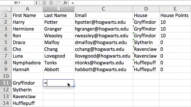
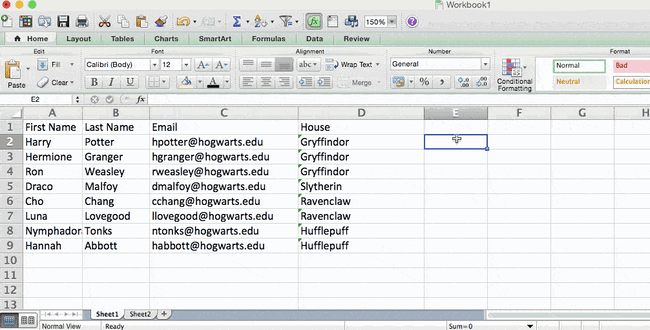
For example, in the situation below, I want to award ten points to everyone who belongs in the Gryffindor house. Instead of manually typing in 10’s next to each Gryffindor student’s name, I can use the IF Excel formula to say that if the student is in Gryffindor, then they should get ten points.
The formula is: IF(logical_test, value_if_true, [value_if_false])
Example Shown Below: =IF(D2=»Gryffindor»,»10″,»0″)
In general terms, the formula would be IF(Logical Test, value of true, value of false). Let’s dig into each of these variables.
- Logical_Test: The logical test is the «IF» part of the statement. In this case, the logic is D2=»Gryffindor» because we want to make sure that the cell corresponding with the student says «Gryffindor.» Make sure to put Gryffindor in quotation marks here.
- Value_if_True: This is what we want the cell to show if the value is true. In this case, we want the cell to show «10» to indicate that the student was awarded the 10 points. Only use quotation marks if you want the result to be text instead of a number.
- Value_if_False: This is what we want the cell to show if the value is false. In this case, for any student not in Gryffindor, we want the cell to show «0». Only use quotation marks if you want the result to be text instead of a number.
Note: In the example above, I awarded 10 points to everyone in Gryffindor. If I later wanted to sum the total number of points, I wouldn’t be able to because the 10’s are in quotes, thus making them text and not a number that Excel can sum.
The real power of the IF function comes when you string multiple IF statements together, or nest them. This allows you to set multiple conditions, get more specific results, and ultimately organize your data into more manageable chunks.
Ranges are one way to segment your data for better analysis. For example, you can categorize data into values that are less than 10, 11 to 50, or 51 to 100. Here’s how that looks in practice:
=IF(B3<11,“10 or less”,IF(B3<51,“11 to 50”,IF(B3<100,“51 to 100”)))
It can take some trial-and-error, but once you have the hang of it, IF formulas will become your new Excel best friend.
11. Use dollar signs to keep one cell’s formula the same regardless of where it moves.
Have you ever seen a dollar sign in an Excel formula? When used in a formula, it isn’t representing an American dollar; instead, it makes sure that the exact column and row are held the same even if you copy the same formula in adjacent rows.
You see, a cell reference — when you refer to cell A5 from cell C5, for example — is relative by default. In that case, you’re actually referring to a cell that’s five columns to the left (C minus A) and in the same row (5). This is called a relative formula. When you copy a relative formula from one cell to another, it’ll adjust the values in the formula based on where it’s moved. But sometimes, we want those values to stay the same no matter whether they’re moved around or not — and we can do that by turning the formula into an absolute formula.
To change the relative formula (=A5+C5) into an absolute formula, we’d precede the row and column values by dollar signs, like this: (=$A$5+$C$5). (Learn more on Microsoft Office’s support page here.)
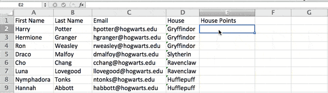
12. Use the VLOOKUP function to pull data from one area of a sheet to another.
Have you ever had two sets of data on two different spreadsheets that you want to combine into a single spreadsheet?
For example, you might have a list of people’s names next to their email addresses in one spreadsheet, and a list of those same people’s email addresses next to their company names in the other — but you want the names, email addresses, and company names of those people to appear in one place.
I have to combine data sets like this a lot — and when I do, the VLOOKUP is my go-to formula.
Before you use the formula, though, be absolutely sure that you have at least one column that appears identically in both places. Scour your data sets to make sure the column of data you’re using to combine your information is exactly the same, including no extra spaces.
The formula: =VLOOKUP(lookup value, table array, column number, Approximate match (TRUE) or Exact match (FALSE))
The formula with variables from our example below: =VLOOKUP(C2,Sheet2!A:B,2,FALSE)
In this formula, there are several variables. The following is true when you want to combine information in Sheet 1 and Sheet 2 onto Sheet 1.
- Lookup Value: This is the identical value you have in both spreadsheets. Choose the first value in your first spreadsheet. In the example that follows, this means the first email address on the list, or cell 2 (C2).
- Table Array: The table array is the range of columns on Sheet 2 you’re going to pull your data from, including the column of data identical to your lookup value (in our example, email addresses) in Sheet 1 as well as the column of data you’re trying to copy to Sheet 1. In our example, this is «Sheet2!A:B.» «A» means Column A in Sheet 2, which is the column in Sheet 2 where the data identical to our lookup value (email) in Sheet 1 is listed. The «B» means Column B, which contains the information that’s only available in Sheet 2 that you want to translate to Sheet 1.
- Column Number: This tells Excel which column the new data you want to copy to Sheet 1 is located in. In our example, this would be the column that «House» is located in. «House» is the second column in our range of columns (table array), so our column number is 2. [Note: Your range can be more than two columns. For example, if there are three columns on Sheet 2 — Email, Age, and House — and you still want to bring House onto Sheet 1, you can still use a VLOOKUP. You just need to change the «2» to a «3» so it pulls back the value in the third column: =VLOOKUP(C2:Sheet2!A:C,3,false).]
- Approximate Match (TRUE) or Exact Match (FALSE): Use FALSE to ensure you pull in only exact value matches. If you use TRUE, the function will pull in approximate matches.
In the example below, Sheet 1 and Sheet 2 contain lists describing different information about the same people, and the common thread between the two is their email addresses. Let’s say we want to combine both datasets so that all the house information from Sheet 2 translates over to Sheet 1.
So when we type in the formula =VLOOKUP(C2,Sheet2!A:B,2,FALSE), we bring all the house data into Sheet 1.
Keep in mind that VLOOKUP will only pull back values from the second sheet that are to the right of the column containing your identical data. This can lead to some limitations, which is why some people prefer to use the INDEX and MATCH functions instead.
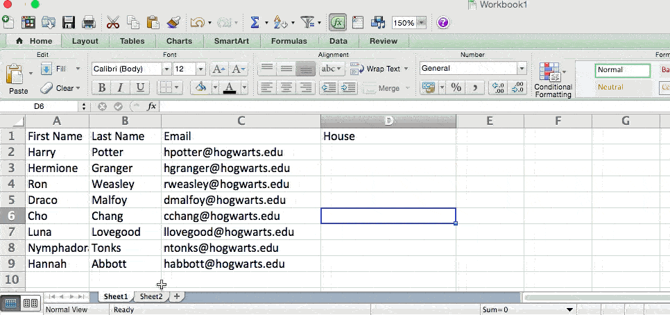
13. Use INDEX and MATCH formulas to pull data from horizontal columns.
Like VLOOKUP, the INDEX and MATCH functions pull in data from another dataset into one central location. Here are the main differences:
- VLOOKUP is a much simpler formula. If you’re working with large data sets that would require thousands of lookups, using the INDEX and MATCH function will significantly decrease load time in Excel.
- The INDEX and MATCH formulas work right-to-left, whereas VLOOKUP formulas only work as a left-to-right lookup. In other words, if you need to do a lookup that has a lookup column to the right of the results column, then you’d have to rearrange those columns in order to do a VLOOKUP. This can be tedious with large datasets and/or lead to errors.
So if I want to combine information in Sheet 1 and Sheet 2 onto Sheet 1, but the column values in Sheets 1 and 2 aren’t the same, then to do a VLOOKUP, I would need to switch around my columns. In this case, I’d choose to do an INDEX and MATCH instead.
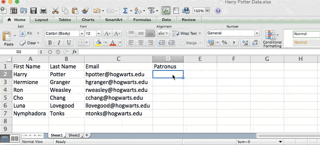
Let’s look at an example. Let’s say Sheet 1 contains a list of people’s names and their Hogwarts email addresses, and Sheet 2 contains a list of people’s email addresses and the Patronus that each student has. (For the non-Harry Potter fans out there, every witch or wizard has an animal guardian called a «Patronus» associated with him or her.) The information that lives in both sheets is the column containing email addresses, but this email address column is in different column numbers on each sheet. I’d use the INDEX and MATCH formulas instead of VLOOKUP so I wouldn’t have to switch any columns around.
So what’s the formula, then? The formula is actually the MATCH formula nested inside the INDEX formula. You’ll see I differentiated the MATCH formula using a different color here.
The formula: =INDEX(table array, MATCH formula)
This becomes: =INDEX(table array, MATCH (lookup_value, lookup_array))
The formula with variables from our example below: =INDEX(Sheet2!A:A,(MATCH(Sheet1!C:C,Sheet2!C:C,0)))
Here are the variables:
- Table Array: The range of columns on Sheet 2 containing the new data you want to bring over to Sheet 1. In our example, «A» means Column A, which contains the «Patronus» information for each person.
- Lookup Value: This is the column in Sheet 1 that contains identical values in both spreadsheets. In the example that follows, this means the «email» column on Sheet 1, which is Column C. So: Sheet1!C:C.
- Lookup Array: This is the column in Sheet 2 that contains identical values in both spreadsheets. In the example that follows, this refers to the «email» column on Sheet 2, which happens to also be Column C. So: Sheet2!C:C.
Once you have your variables straight, type in the INDEX and MATCH formulas in the top-most cell of the blank Patronus column on Sheet 1, where you want the combined information to live.
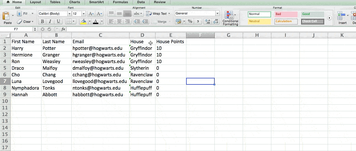
14. Use the COUNTIF function to make Excel count words or numbers in any range of cells.
Instead of manually counting how often a certain value or number appears, let Excel do the work for you. With the COUNTIF function, Excel can count the number of times a word or number appears in any range of cells.
For example, let’s say I want to count the number of times the word «Gryffindor» appears in my data set.
The formula: =COUNTIF(range, criteria)
The formula with variables from our example below: =COUNTIF(D:D,»Gryffindor»)
In this formula, there are several variables:
- Range: The range that we want the formula to cover. In this case, since we’re only focusing on one column, we use «D:D» to indicate that the first and last column are both D. If I were looking at columns C and D, I would use «C:D.»
- Criteria: Whatever number or piece of text you want Excel to count. Only use quotation marks if you want the result to be text instead of a number. In our example, the criteria is «Gryffindor.»
Simply typing in the COUNTIF formula in any cell and pressing «Enter» will show me how many times the word «Gryffindor» appears in the dataset.
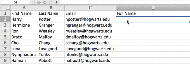
15. Combine cells using &.
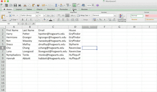
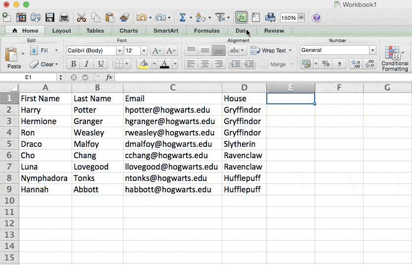
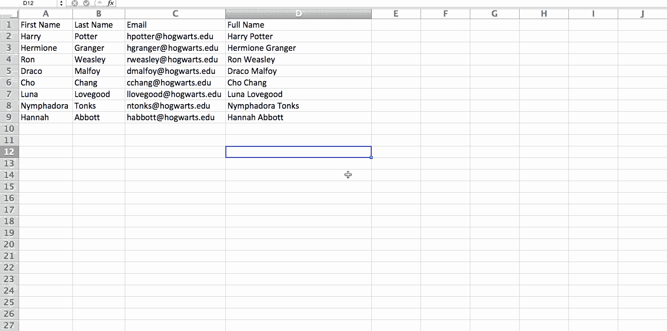
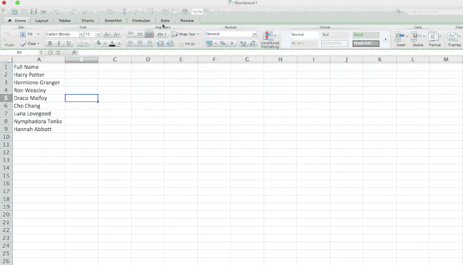
Databases tend to split out data to make it as exact as possible. For example, instead of having a column that shows a person’s full name, a database might have the data as a first name and then a last name in separate columns. Or, it may have a person’s location separated by city, state, and zip code. In Excel, you can combine cells with different data into one cell by using the «&» sign in your function.
The formula with variables from our example below: =A2&» «&B2
Let’s go through the formula together using an example. Pretend we want to combine first names and last names into full names in a single column. To do this, we’d first put our cursor in the blank cell where we want the full name to appear. Next, we’d highlight one cell that contains a first name, type in an «&» sign, and then highlight a cell with the corresponding last name.
But you’re not finished — if all you type in is =A2&B2, then there will not be a space between the person’s first name and last name. To add that necessary space, use the function =A2&» «&B2. The quotation marks around the space tell Excel to put a space in between the first and last name.
To make this true for multiple rows, simply drag the corner of that first cell downward as shown in the example.
16. Add checkboxes.
If you’re using an Excel sheet to track customer data and want to oversee something that isn’t quantifiable, you could insert checkboxes into a column.
For example, if you’re using an Excel sheet to manage your sales prospects and want to track whether you called them in the last quarter, you could have a «Called this quarter?» column and check off the cells in it when you’ve called the respective client.
Here’s how to do it.
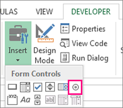
Highlight a cell you’d like to add checkboxes to in your spreadsheet. Then, click DEVELOPER. Then, under FORM CONTROLS, click the checkbox or the selection circle highlighted in the image below.
Once the box appears in the cell, copy it, highlight the cells you also want it to appear in, and then paste it.
17. Hyperlink a cell to a website.
If you’re using your sheet to track social media or website metrics, it can be helpful to have a reference column with the links each row is tracking. If you add a URL directly into Excel, it should automatically be clickable. But, if you have to hyperlink words, such as a page title or the headline of a post you’re tracking, here’s how.
Highlight the words you want to hyperlink, then press Shift K. From there a box will pop up allowing you to place the hyperlink URL. Copy and paste the URL into this box and hit or click Enter.
If the key shortcut isn’t working for any reason, you can also do this manually by highlighting the cell and clicking Insert > Hyperlink.
18. Add drop-down menus.
Sometimes, you’ll be using your spreadsheet to track processes or other qualitative things. Rather than writing words into your sheet repetitively, such as «Yes», «No», «Customer Stage», «Sales Lead», or «Prospect», you can use dropdown menus to quickly mark descriptive things about your contacts or whatever you’re tracking.
Here’s how to add drop-downs to your cells.
Highlight the cells you want the drop-downs to be in, then click the Data menu in the top navigation and press Validation.
From there, you’ll see a Data Validation Settings box open. Look at the Allow options, then click Lists and select Drop-down List. Check the In-Cell dropdown button, then press OK.
19. Use the format painter.
As you’ve probably noticed, Excel has a lot of features to make crunching numbers and analyzing your data quick and easy. But if you ever spent some time formatting a sheet to your liking, you know it can get a bit tedious.
Don’t waste time repeating the same formatting commands over and over again. Use the format painter to easily copy the formatting from one area of the worksheet to another. To do so, choose the cell you’d like to replicate, then select the format painter option (paintbrush icon) from the top toolbar.
Excel Keyboard Shortcuts
Creating reports in Excel is time-consuming enough. How can we spend less time navigating, formatting, and selecting items in our spreadsheet? Glad you asked. There are a ton of Excel shortcuts out there, including some of our favorites listed below.
Create a New Workbook
PC: Ctrl-N | Mac: Command-N
Select Entire Row
PC: Shift-Space | Mac: Shift-Space
Select Entire Column
PC: Ctrl-Space | Mac: Control-Space
Select Rest of Column
PC: Ctrl-Shift-Down/Up | Mac: Command-Shift-Down/Up
Select Rest of Row
PC: Ctrl-Shift-Right/Left | Mac: Command-Shift-Right/Left
Add Hyperlink
PC: Ctrl-K | Mac: Command-K
Open Format Cells Window
PC: Ctrl-1 | Mac: Command-1
Autosum Selected Cells
PC: Alt-= | Mac: Command-Shift-T
Other Excel Help Resources
- How to Make a Chart or Graph in Excel [With Video Tutorial]
- Design Tips to Create Beautiful Excel Charts and Graphs
- Totally Free Microsoft Excel Templates That Make Marketing Easier
- How to Learn Excel Online: Free and Paid Resources for Excel Training
Use Excel to Automate Processes in Your Team
Even if you’re not an accountant, you can still use Excel to automate tasks and processes in your team. With the tips and tricks we shared in this post, you’ll be sure to use Excel to its fullest extent and get the most out of the software to grow your business.
Editor’s Note: This post was originally published in August 2017 but has been updated for comprehensiveness.

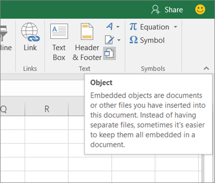
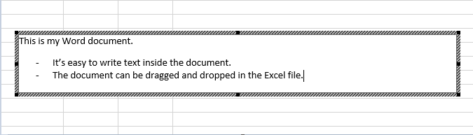
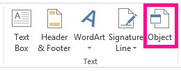
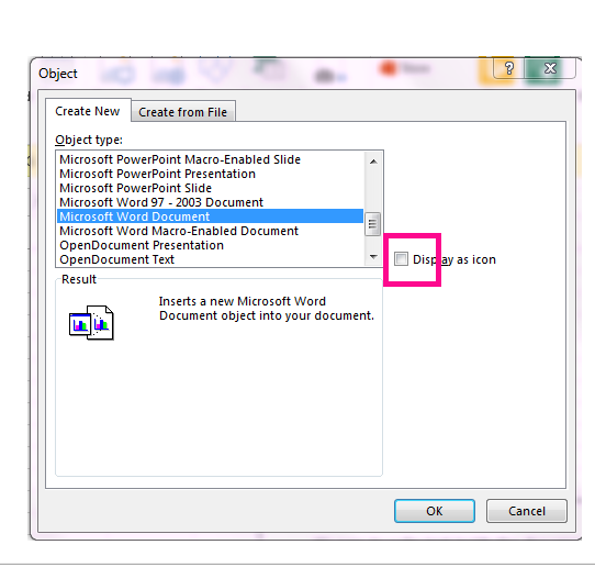
You can use Object Linking and Embedding (OLE) to include content from other programs, such as Word or Excel.
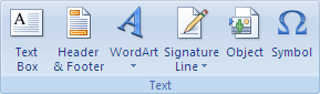
OLE is supported by many different programs, and OLE is used to make content that is created in one program available in another program. For example, you can insert an Office Word document in an Office Excel workbook. To see what types of content that you can insert, click Object in the Text group on the Insert tab. Only programs that are installed on your computer and that support OLE objects appear in the Object type box.
If you copy information between Excel or any program that supports OLE, such as Word, you can copy the information as either a linked object or an embedded object. The main differences between linked objects and embedded objects are where the data is stored and how the object is updated after you place it in the destination file. Embedded objects are stored in the workbook that they are inserted in, and they are not updated. Linked objects remain as separate files, and they can be updated.
Linked and embedded objects in a document
1. An embedded object has no connection to the source file.
2. A linked object is linked to the source file.
3. The source file updates the linked object.
When to use linked objects
If you want the information in your destination file to be updated when the data in the source file changes, use linked objects.
With a linked object, the original information remains stored in the source file. The destination file displays a representation of the linked information but stores only the location of the original data (and the size if the object is an Excel chart object). The source file must remain available on your computer or network to maintain the link to the original data.
The linked information can be updated automatically if you change the original data in the source file. For example, if you select a paragraph in a Word document and then paste the paragraph as a linked object in an Excel workbook, the information can be updated in Excel if you change the information in your Word document.
When to use embedded objects
If you don’t want to update the copied data when it changes in the source file, use an embedded object. The version of the source is embedded entirely in the workbook. If you copy information as an embedded object, the destination file requires more disk space than if you link the information.
When a user opens the file on another computer, he can view the embedded object without having access to the original data. Because an embedded object has no links to the source file, the object is not updated if you change the original data. To change an embedded object, double-click the object to open and edit it in the source program. The source program (or another program capable of editing the object) must be installed on your computer.
Changing the way that an OLE object is displayed
You can display a linked object or embedded object in a workbook exactly as it appears in the source program or as an icon. If the workbook will be viewed online, and you don’t intend to print the workbook, you can display the object as an icon. This minimizes the amount of display space that the object occupies. Viewers who want to display the information can double-click the icon.
Embed an object in a worksheet
-
Click inside the cell of the spreadsheet where you want to insert the object.
-
On the Insert tab, in the Text group, click Object
 .
. -
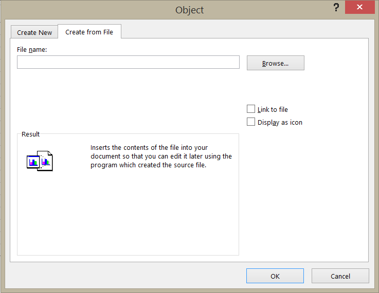
In the Object dialog box, click the Create from File tab.
-
Click Browse, and select the file you want to insert.
-
If you want to insert an icon into the spreadsheet instead of show the contents of the file, select the Display as icon check box. If you don’t select any check boxes, Excel shows the first page of the file. In both cases, the complete file opens with a double click. Click OK.
Note: After you add the icon or file, you can drag and drop it anywhere on the worksheet. You can also resize the icon or file by using the resizing handles. To find the handles, click the file or icon one time.
 .
.
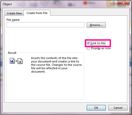
Insert a link to a file
You might want to just add a link to the object rather than fully embedding it. You can do that if your workbook and the object you want to add are both stored on a SharePoint site, a shared network drive, or a similar location, and if the location of the files will remain the same. This is handy if the linked object undergoes changes because the link always opens the most up-to-date document.
Note: If you move the linked file to another location, the link won’t work anymore.
-
Click inside the cell of the spreadsheet where you want to insert the object.
-
On the Insert tab, in the Text group, click Object
. -
Click the Create from File tab.
-
Click Browse, and then select the file you want to link.
-
Select the Link to file check box, and click OK.
Create a new object from inside Excel
You can create an entirely new object based on another program without leaving your workbook. For example, if you want to add a more detailed explanation to your chart or table, you can create an embedded document, such as a Word or PowerPoint file, in Excel. You can either set your object to be displayed right in a worksheet or add an icon that opens the file.
-
Click inside the cell of the spreadsheet where you want to insert the object.
-
On the Insert tab, in the Text group, click Object
. -
On the Create New tab, select the type of object you want to insert from the list presented. If you want to insert an icon into the spreadsheet instead of the object itself, select the Display as icon check box.
-
Click OK. Depending on the type of file you are inserting, either a new program window opens or an editing window appears within Excel.
-
Create the new object you want to insert.
When you’re done, if Excel opened a new program window in which you created the object, you can work directly within it.
When you’re done with your work in the window, you can do other tasks without saving the embedded object. When you close the workbook your new objects will be saved automatically.
Note: After you add the object, you can drag and drop it anywhere on your Excel worksheet. You can also resize the object by using the resizing handles. To find the handles, click the object one time.
Embed an object in a worksheet
-
Click inside the cell of the spreadsheet where you want to insert the object.
-
On the Insert tab, in the Text group, click Object.
-
Click the Create from File tab.
-
Click Browse, and select the file you want to insert.
-
If you want to insert an icon into the spreadsheet instead of show the contents of the file, select the Display as icon check box. If you don’t select any check boxes, Excel shows the first page of the file. In both cases, the complete file opens with a double click. Click OK.
Note: After you add the icon or file, you can drag and drop it anywhere on the worksheet. You can also resize the icon or file by using the resizing handles. To find the handles, click the file or icon one time.
Insert a link to a file
You might want to just add a link to the object rather than fully embedding it. You can do that if your workbook and the object you want to add are both stored on a SharePoint site, a shared network drive, or a similar location, and if the location of the files will remain the same. This is handy if the linked object undergoes changes because the link always opens the most up-to-date document.
Note: If you move the linked file to another location, the link won’t work anymore.
-
Click inside the cell of the spreadsheet where you want to insert the object.
-
On the Insert tab, in the Text group, click Object.
-
Click the Create from File tab.
-
Click Browse, and then select the file you want to link.
-
Select the Link to file check box, and click OK.
Create a new object from inside Excel
You can create an entirely new object based on another program without leaving your workbook. For example, if you want to add a more detailed explanation to your chart or table, you can create an embedded document, such as a Word or PowerPoint file, in Excel. You can either set your object to be displayed right in a worksheet or add an icon that opens the file.
-
Click inside the cell of the spreadsheet where you want to insert the object.
-
On the Insert tab, in the Text group, click Object.
-
On the Create New tab, select the type of object you want to insert from the list presented. If you want to insert an icon into the spreadsheet instead of the object itself, select the Display as icon check box.
-
Click OK. Depending on the type of file you are inserting, either a new program window opens or an editing window appears within Excel.
-
Create the new object you want to insert.
When you’re done, if Excel opened a new program window in which you created the object, you can work directly within it.
When you’re done with your work in the window, you can do other tasks without saving the embedded object. When you close the workbook your new objects will be saved automatically.
Note: After you add the object, you can drag and drop it anywhere on your Excel worksheet. You can also resize the object by using the resizing handles. To find the handles, click the object one time.
Link or embed content from another program by using OLE
You can link or embed all or part of the content from another program.
Create a link to content from another program
-
Click in the worksheet where you want to place the linked object.
-
On the Insert tab, in the Text group, click Object.
-
Click the Create from File tab.
-
In the File name box, type the name of the file, or click Browse to select from a list.
-
Select the Link to file check box.
-
Do one of the following:
-
To display the content, clear the Display as icon check box.
-
To display an icon, select the Display as icon check box. Optionally, to change the default icon image or label, click Change Icon, and then click the icon that you want from the Icon list, or type a label in the Caption box.
Note: You cannot use the Object command to insert graphics and certain types of files. To insert a graphic or file, on the Insert tab, in the Illustrations group, click Picture.
-
Embed content from another program
-
Click in the worksheet where you want to place the embedded object.
-
On the Insert tab, in the Text group, click Object.
-
If the document does not already exist, click the Create New tab. In the Object type box, click the type of object that you want to create.
If the document already exists, click the Create from File tab. In the File name box, type the name of the file, or click Browse to select from a list.
-
Clear the Link to file check box.
-
Do one of the following:
-
To display the content, clear the Display as icon check box.
-
To display an icon, select the Display as icon check box. To change the default icon image or label, click Change Icon, and then click the icon that you want from the Icon list, or type a label in the Caption box.
-
Link or embed partial content from another program
-
From a program other than Excel, select the information that you want to copy as a linked or embedded object.
-
On the Home tab, in the Clipboard group, click Copy.
-
Switch to the worksheet that you want to place the information in, and then click where you want the information to appear.
-
On the Home tab, in the Clipboard group, click the arrow below Paste, and then click Paste Special.
-
Do one of the following:
-
To paste the information as a linked object, click Paste link.
-
To paste the information as an embedded object, click Paste. In the As box, click the entry with the word «object» in its name. For example, if you copied the information from a Word document, click Microsoft Word Document Object.
-

Change the way that an OLE object is displayed
-
Right-click the icon or object, point to object typeObject (for example, Document Object), and then click Convert.
-
Do one of the following:
-
To display the content, clear the Display as icon check box.
-
To display an icon, select the Display as icon check box. Optionally, you can change the default icon image or label. To do that, click Change Icon, and then click the icon that you want from the Icon list, or type a label in the Caption box.
-
Control updates to linked objects
You can set links to other programs to be updated in the following ways: automatically, when you open the destination file; manually, when you want to see the previous data before updating with the new data from the source file; or when you specifically request the update, regardless of whether automatic or manual updating is turned on.
Set a link to another program to be updated manually
-
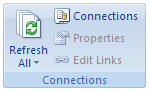
On the Data tab, in the Connections group, click Edit Links.
Note: The Edit Links command is unavailable if your file does not contain links to other files.
-
In the Source list, click the linked object that you want to update. An A in the Update column means that the link is automatic, and an M in the Update column means that the link is set to Manual update.
Tip: To select multiple linked objects, hold down CTRL and click each linked object. To select all linked objects, press CTRL+A.
-
To update a linked object only when you click Update Values, click Manual.
Set a link to another program to be updated automatically
-
On the Data tab, in the Connections group, click Edit Links.
Note: The Edit Links command is unavailable if your file does not contain links to other files.
-
In the Source list, click the linked object that you want to update. An A in the Update column means that the link will update automatically, and an M in the Update column means that the link must be updated manually.
Tip: To select multiple linked objects, hold down CTRL and click each linked object. To select all linked objects, press CTRL+A.
-
Click OK.
Issue: I can’t update the automatic links on my worksheet
The Automatic option can be overridden by the Update links to other documents Excel option.
To ensure that automatic links to OLE objects can be automatically updated:
-
Click the Microsoft Office Button
, click Excel Options, and then click the Advanced category. -
Under When calculating this workbook, make sure that the Update links to other documents check box is selected.
 , click Excel Options, and then click the Advanced category.
Update a link to another program now
-
On the Data tab, in the Connections group, click Edit Links.
Note: The Edit Links command is unavailable if your file does not contain linked information.
-
In the Source list, click the linked object that you want to update.
Tip: To select multiple linked objects, hold down CTRL and click each linked object. To select all linked objects, press CTRL+A.
-
Click Update Values.
Edit content from an OLE program
While you are in Excel, you can change the content linked or embedded from another program.
Edit a linked object in the source program
-
On the Data tab, in the Connections group, click Edit Links.
Note: The Edit Links command is unavailable if your file does not contain linked information.
-
In the Source file list, click the source for the linked object, and then click Open Source.
-
Make the changes that you want to the linked object.
-
Exit the source program to return to the destination file.
Edit an embedded object in the source program
-
Double-click the embedded object to open it.
-
Make the changes that you want to the object.
-
If you are editing the object in place within the open program, click anywhere outside of the object to return to the destination file.
If you edit the embedded object in the source program in a separate window, exit the source program to return to the destination file.
Note: Double-clicking certain embedded objects, such as video and sound clips, plays the object instead of opening a program. To edit one of these embedded objects, right-click the icon or object, point to object typeObject (for example, Media Clip Object), and then click Edit.
Edit an embedded object in a program other than the source program
-
Select the embedded object that you want to edit.
-
Right-click the icon or object, point to object typeObject (for example, Document Object), and then click Convert.
-
Do one of the following:
-
To convert the embedded object to the type that you specify in the list, click Convert to.
-
To open the embedded object as the type that you specify in the list without changing the embedded object type, click Activate.
-
Select an OLE object by using the keyboard
-
Press CTRL+G to display the Go To dialog box.
-
Click Special, select Objects, and then click OK.
-
Press TAB until the object that you want is selected.
-
Press SHIFT+F10.
-
Point to Object or Chart Object, and then click Edit.
Issue: When I double-click a linked or embedded object, a «cannot edit» message appears
This message appears when the source file or source program can’t be opened.
Make sure that the source program is available If the source program is not installed on your computer, convert the object to the file format of a program that you do have installed.
Ensure that memory is adequate Make sure that you have enough memory to run the source program. Close other programs to free up memory, if necessary.
Close all dialog boxes If the source program is running, make sure that it doesn’t have any open dialog boxes. Switch to the source program, and close any open dialog boxes.
Close the source file If the source file is a linked object, make sure that another user doesn’t have it open.
Ensure that the source file name has not changed If the source file that you want to edit is a linked object, make sure that it has the same name as it did when you created the link and that it has not been moved. Select the linked object, and then click the Edit Links command in the Connections group on the Data tab to see the name of the source file. If the source file has been renamed or moved, use the Change Source button in the Edit Links dialog box to locate the source file and reconnect the link.
Need more help?
You can always ask an expert in the Excel Tech Community or get support in the Answers community.
Subjects>Electronics>Computers

Wiki User
∙ 13y ago
Best Answer
![]() Copy
Copy
Excel creates spreadsheet documents. The documents are known as
workbooks, and a workbook contains worksheets.
Wiki User
∙ 13y ago
This answer is:
![]()
Study guides
Add your answer:
![]() Earn +
Earn +
20
pts
Q: What document can you create in Excel?
Write your answer…
Submit
Still have questions?
![]()
![]()
Related questions
People also asked
What are the uses of MS Excel in daily life? And also in businesses too. Well, there are a lot. Nowadays, people are in a hurry. They need to perform various operations in their daily life. But to perform these operations, they need to do some calculations. So how can they perform calculations easily? The most effective answer to this question is the use of excel.
Excel helps individuals and businesses to perform difficult calculations in no time. MS Excel is the most famous spreadsheet software in the world. In this blog, we will discuss various uses of excel in our life. But before we get started with the uses of Excel, let’s have a look at what MS Excel is.
However, if you are looking for Excel assignment help, then don’t worry. At statanalytica.com, we provide the best Excel assignment help at an affordable price. So, don’t waste your time get the help now!
MS Excel
MS Excel is one of the major parts of the MS office suite.
It is one of the most powerful spreadsheet software in the world.
The spreadsheet contains a table with various numbers of rows and columns.
These rows and columns are used to put the values.
You can easily manipulate these values using some complex arithmetic operations with the help of excel formulas.
Apart from that, MS Excel also offers programming support, which makes it better than other spreadsheet software.
You can do the programming with excel via Microsoft Visual Basic for Applications. On the other hand, there are many excel project ideas that you can use to improve your skills.
It also has the ability to get data from external sources via Microsoft’s Dynamic Data Exchange.
Apart from that, it also offers extensive graphic support to the users.
The most common uses of MS excel are performing basic calculations, creating pivot tables, and creating macros.

Importance Of MS Excel In Our Daily Life And Business Life
Following are some importance of Excel that are related to our daily life and business lives.
1. Easy Computation Solutions
MS Excel has the ability to do several numbers of arithmetic calculations. With the help of different formulas, it can add, multiply, subtract, and divide lots of numbers simultaneously. Moreover, it can easily be re-do if the value is changed or added.
2. Options Of Formatting
Excel has various formatting options, like highlighting, italics, colors, etc., that enable businesses to show and bring out the essential data differently.
3. Availability Of Online Access
MS Excel is part of the Office 365 productivity Suite. It means businesses’ employers and employees can easily access their files over the cloud network.
4. Analysis Charts
MS Excel enables its users to create analysis charts easily. You can create Pie charts or Clustered Columns by filtering and correctly inputting data in just a few clicks. Even Excel allows you to customize the colors and boundaries of the diagrams.
5. All Data At One Place
Excel contains over 10 lakh rows and 16 thousand columns in the spreadsheet. You can also import data, add pictures and other objects through the insert tab. Excel enables you to put all the data you collected from different files in one place easily.
Now let’s move on to the uses of Excel in our daily life. Here we go:-
USES OF EXCEL: 8 Important Uses Of Microsoft Excel
1. Education
There are various uses of MS Excel in education. Even Excel is making teaching a lot easier for teachers.
The teachers use tables, shapes, charts, and other tools in excel to present the topics to the students.
Moreover, the teachers are also using formulas to teach the students about mathematical computations.
In education, the data visualization of MS excel is the key to the teachers.
Now the students can easily understand the topic because of the visualization, especially when the teachers are going to represent the stats, then they use bars and charts.
Apart from that, the use of MS Excel in schools and colleges to create timetables.
There are various pre-built templates in MS excel.
You can use these templates to create the timetable.
Besides, excel also offers formulas that are useful for multiple education purposes.
It is one of the best uses of Excel.
You can use these templates to create the timetable.
Besides, excel also offers formulas that are useful for multiple education purposes.
2. Business
Excel plays a crucial role in business. Even every business owner is using excel.
The use of excel in business varies from organization to organization.
The business can use MS Excel to perform goal setting, budgeting process, and planning, etc.
Now the business can easily manage their daily operations because of excel.
Apart from that, they are also able to predict their performance.
The excel financial formulas are doing a tremendous job for the business.
MS Excel is offering the IF formula, which is quite helpful in creating hundreds of logic in the business calculations.
MS Excel is quite handy for business operations.
All you need to do is visit the template menu to take full advantage of it.
The best part of the pre-built template is, you need not create anything from scratch.
3. Goal Setting and Planning
We all have daily goals or weekly goals.
Therefore to manage our daily tasks for the goals. We can use MS excel.
In MS Excel, all we need to do is accomplish the daily task along with the remark column.
Whenever we complete our daily tasks, we write on the remark columns that we are done with the task.
It is also helpful for planning purposes.
With the help of excel, we can calculate everything in advance as part of our planning.
4. Business Owners
The previous point highlighted the use of MS Excel for business.
But at this point, we will share with you the uses of MS Excel for business owners.
We know that business owners also need to perform various tasks from their end.
Some of these tasks are work progress, team management, and payouts details, etc.
One of the significant tasks for the business owner is to track the marketing campaign progress. However, if you have any pending marketing homework help then you can get our marketing help at a very affordable price.
Excel makes it simple and easy for business owners.
All they need to do is select the prebuilt template to start creating the sheet.
5. Housewives
It helps housewives to manage their daily expenses as well as grocery.
With the use of excel, they can create the report for weekly and monthly expenses.
It also helps them to track their expenses.
Most housewives are also helping their children to learn the basic skills of MS Excel.
In this way, the statistics students also get ready from the beginning of the academics.
Apart from that, Excel knowledge also emerges from housewives to earn a possessive income.
There are lots of part-time jobs available for housewives.
It is one of the best uses of Excel.
Also, Read
- Excel vs Quickbooks; Best Points You Need To Know
- How to Find Z Score in Excel | Best Ways to Find it Like A Pro
- A Guide On Frequency Distribution Excel For Beginners
6. Data Analysis And Data Science
Data analysis is one of the most emerging fields in the business perspective.
The business needs to perform various operations on the data.
The reason is companies are not using a single source.
They use multiple sources such as their blog, eCommerce sites, social media, offline data, and more.
All these jobs need time and energy. Sometimes it becomes overwhelming for the business to manage the data. In this case, excel plays a crucial role in the business.
Excel offers the filter function, which is quite handy for the data analyst to understand the data. Nowadays, excel is also used in the field of data science.
There are lots of functions that are helping in Big Data technologies.
The programming features of Excel with VBA make it one of the best options for data science technologies.
There are lots of operations that can be performed with the use of excel.
7. Daily Progress Report
Excel is also helpful in creating a daily progress report. Most of the companies track their daily progress with the help of excel.
Especially in project-based companies where the clients need a weekly report from the company.
For this, the company uses the daily progress report to showcase the daily work progress to the client.
Excel offers the table with the date and time.
You can also add the manual columns such as client, tasks, duration, and status as per the business requirements.
Apart from the companies, the daily progress report is also helpful in academics.
The teachers and the students can track their daily progress with the help of excel.
It is one of the best uses of Excel.
8. Career Development
When we talk about career development.
MS Excel is also playing a crucial role in this sector. Excel teaches you the most prominent skills of management.
With the help of excel, we try to calculate everything in advance.
Because in our life, we need to perform various calculations to run our daily life.
If you get good command over MS Excel, you are also eligible to get the best job in data analytics or data science.
Excel helps you in career management, time management, learning management, life management, and so on.If you are a student, then you can manage all your expenses with the help of excel.
5 Uses Of MS Excel In Businesses
At a very basic level, MS Excel is used for storing, analyzing, sorting, and reporting. However, it is extremely popular in businesses because it is fairly easy to use.
1. Business Analysis
Excel is used to do business analysis. Through this, businesses make decisions with collected data. Generally, companies gather data on a daily basis that is related to product sales, website traffic, insurance claim, etc.
2. People Management
It is one of the top uses of Excel in businesses. MS Excel is a powerful way to collect information about people. Through excel, personal information of employees, customers, supporters, etc., can be stored and recovered efficiently.
3. Managing Operations
Excel is heavily dependent on the daily operations of numerous businesses. Business activities generally involve complex logistics. Inventory flows require to be managed, so that company’s operations run smoothly. In simple words, keeping track of supplier and client transactions, listing critical dates, and managing times and schedules. It is only possible through MS Excel.
4. Report Of Performance
MS Excel can do monitoring and reporting of performance effectively. A simple way to transform data into a performance report in Excel is to build a pivot table. By creating a pivot table and linking it to data, you can get extra useful information from the dataset. If you need to analyze huge volumes of data then will probably be easier to connect this dataset with a reporting tool.
5. Office Administration
MS Excel stores and enters the administrative data. Then this data is used for accounting and financial reporting and business analysis, and performance reporting. Moreover, Excel supports office administration in daily tasks such as invoicing, paying bills, etc.
Top 5 Cool Things You Can Try Right Now Using Excel
You can’t ignore Excel’s important role in daily work because it deals with big data. However, many useful tips and tricks for beginners and advanced users are still inevitably overlooked. Here are five cool things you can try right now using Excel.
1. Play with numbers
Excel’s main function is to work with numbers. Excel makes sorting, retrieving, and analyzing a huge (or even small!) quantity of data a breeze.
When it comes to using Excel for anything numbers-related, there are a few general categories to keep in mind.
Calculation:
Do you ever find yourself repeating the same calculations? You may create a completely personalized calculator by programming your frequently used formulae in Excel. That way, all you have to do is type in your numbers, and Excel will calculate the result for you—no effort necessary. Isn’t it cool?
Charts:
The number of pie charts, line charts, scatter charts, bar charts, area charts, and column charts is endless. Excel can turn rows and columns of figures into attractive charts. And it is sure to become one of your favorite features if you need to convey data in a more visual and consumable way.
2. Making Plans
Let’s get away from the numbers for a moment —Excel can help you plan and organise a lot of things that don’t require multiple rows of figures.
Worksheet for goal setting:
Excel always helps to have something to keep you focused and on track. And it would either it’s career objectives, fitness goals, or money goals. You may use excel to build a variety of spreadsheets, logs, and planning papers to track your progress and, ideally, cross the finish line.
Schedules and calendars:
Do you need to create a content schedule for your blog or website? Are you looking for lesson plans for your classroom? Do you or your family have a daily schedule? Excel may be surprisingly powerful when it comes to multiple calendars. Try this today to schedule your work.
3. Involving Others
Do you need to get information from others? One method is to use survey tools and forms. But, don’t worry, you can make them all in your own Excel.
Quizzes:
Are you trying to assess someone else’s — or even your own — for the understanding of a topic? You may create a bank of questions and answers in one worksheet and then have Excel quiz you in another.
Forms:
Excel is an excellent tool for designing forms. And it starts from basic to complex. You may even create numerous drop-down menus so that users can choose from a predefined list of options.
4. Getting things done
Do you want to increase your productivity? Excel can easily come to your rescue with various functions that can help you manage your tasks and to-dos with simplicity.
Timesheets:
You already know that keeping track of your time may help you be more productive. There are many attractive applications and tools to help you in meeting these demands. Consider Excel as the actual time-tracking tool. It continues to be a possible alternative to time sheets today.
Checklist:
Similarly, you may make a basic checklist to cross off the items you’ve bought or completed. And it can be related to a shopping list to a list of to-dos for planned marketing tasks.
5. Excel just for fun.
With the help of excel, you can do a variety of other interesting things for fun.
Cloud of words:
Word clouds are not the most scientific way to describe facts. However, they are a fun (not to mention attractive) method to determine which words are used the most. You guessed it—Excel can be used to make one.
Logbooks from the past:
Whether you want to keep track of the different tasks you have completed, the exercises you have done, or something else completely, Excel is what you have for sorting and logging those things.
3 Powerful Excel Functions That Make Work
The following are the most useful functions that we can use in our daily life.
1. The SUM Function
This function is the most used function when it comes to computing data on Excel. This function is used to sum a group of numbers in a specific set of cells.
It means you do not need to type a long cumbrous formula to calculate the sum of the data.
The SUM function is performed by typing the formula on the function bar, highlighting the cells you want to add, and pressing “ENTER”.
- The Syntax formula for SUM function is “=SUM(Cell numbers)”.
- You can also use the Σ symbol to add the data you need.
- Moreover, “ALT+” also helps to add the numbers.
2. The TEXT Function
The TEXT function is a useful tool that helps in converting the date or numbers into a text string in a particular format. Keep in mind the text formula only works to convert numeric values to text.
The TEXT function’ formula is =”Text” (Value, format_text).
Value refers to the particular number you want to convert to text.
Format_text refers to the format of the conversion.
3. The AVERAGE Function
The AVERAGE function is used for getting the average of the data. As the function of SUM, it is commonly used in computing and analyzing the data on the spreadsheet.
The syntax formula for the AVERAGE function is “=AVERAGE(Cell number).
Some Of The Documents That You Can Create in Excel
Microsoft Excel is a versatile software that allows users to create various documents. Here is the list of some of the documents that you can create in excel, which are as follows:
1. Spreadsheets
Excel is primarily used for creating spreadsheets, which are documents that organize and analyze data in rows and columns. Spreadsheets can be used for budgeting, financial analysis, inventory management, and more.
2. Charts and graphs
Excel allows users to create charts and graphs to visualize data, such as bar charts, line charts, pie charts, and scatter plots.
3. Calendars
Excel can create calendars for scheduling appointments, meetings, or events.
4. Invoices
Excel can create invoices with item descriptions, prices, taxes, and totals.
5. Budgets
Excel is useful for creating personal or business budgets, where users can track their expenses and income.
6. Forms
Excel can be used to create forms for data collection, such as surveys or questionnaires.
7. Project plans
Excel can create project plans, including timelines, budgets, and resource allocation.
8. Gantt charts
Excel allows users to create Gantt charts and visual representations of project schedules that help track progress and identify potential issues.
9. Data entry forms
Excel can create forms that make it easier to input and organize data.
10. Contact lists
Excel can create lists that include names, addresses, phone numbers, and other relevant information.
Well, these are some of the documents you can try and make in excel.
Conclusion
The more you learn, the more you can earn with excel. The same philosophy applies to MS excel.
If you develop your excel skills to the peak level, you are eligible to get reputed jobs in analytics.
As we have seen, there are lots of uses for excel. But here, we have mentioned a few.
There are many more uses to excel in the world. Excel makes life easier for us.
Now we can perform a complete calculation without having a strong command of math and statistics.
All this becomes possible only because of MS excel. So don’t be the one who is not aware of MS excel.
Start learning excel today from the experts.
Also, get the best excel assignment help from MS excel experts at nominal charges.
FAQs
Q1. What is Excel used for?
Excel is generally used to manage data and perform financial analysis. On the other hand, it is used in every business and company of all sizes. The main uses of Excel include:
1. Customer relationship management (CRM)
2. Time management
3. Task management
4. Data entry
5. Data management
6. Financial modeling
7. Accounting
8. Financial analysis
9. Charting and graphing
10. Programming
11. You can do almost anything that needs to be organized!
Q2. What are the benefits of MS Excel in your life as a student?
The benefits of Excel in student’s lives are as follows:
1. The Best way to store data.
2. Able to perform calculations
3. Every tool for data analysis
4. Print report easily
5. Transform and clear data
Q3. What are the three most common uses for Excel?
The three most common uses for MS Excel are creating budgets, producing graphs and charts, and storing and sorting the data.