
Contents
- Tools, Calculators and Simulations
- Dashboards and Reports with Charts
- Automate Jobs with VBA macros
- Solver Add-in & Statistical Analysis
- Data Entry and Lists
- Games in Excel!
- Educational use with Interactive features
- Create Cheatsheets with Excel
- Diagrams, Mockups, Gantt Charts
- Fetch live data from web
- Excel as a Database
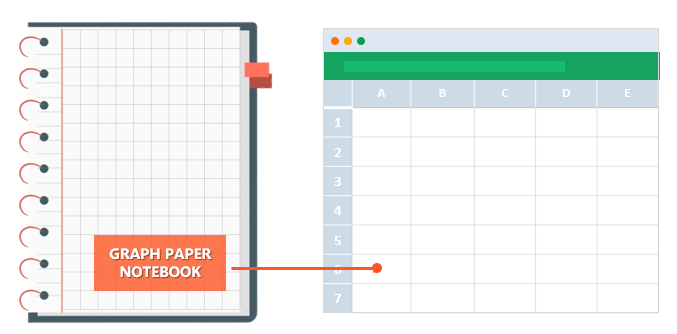
Excel is one of the most used software in today’s digital world. Most people quickly open up an Excel file when they need to write or calculate anything. It is like “paper”. (remember those graph notebooks from school times..)
Actually, this is not only specific to Microsoft’s Excel but most of the spreadsheet software like open office or google sheets. However, we will focus on Excel and what can you do with it today, as it offers huge flexibility you will discover below.
Let’s start with the main usage areas of Excel. As we all know, spreadsheets are designed to make calculations easier. So they contain “formulas”. They allow us to make basic math like summing, multiplying, finding average as well as advanced calculations like regression analysis, conversions, and so on.
When we combine these powerful math features with some tables, lists, or other UI elements, we can come up with a calculator. And most of the time they will be dynamic (meaning that when you change a parameter all the rest of the calculations will adapt accordingly)
Below see an example from our past studies as Someka:
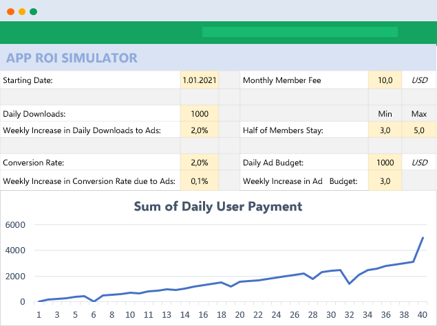
We have built this calculator for an app development company executive. He was changing the parameters he wants and sees the outcomes immediately.
This is great especially when you try to make big “models” in excel. Financial Modeling is one of the most used application areas of these big models. If we tried to do this with pen-paper (which used to be the way once upon a time) it would be horrible I guess:

Financial modeling is also being used to test the excel skills of experts. They even make a competition for it: ModelOff
We also have a tool for startups to make a feasibility study playing with their own variables:
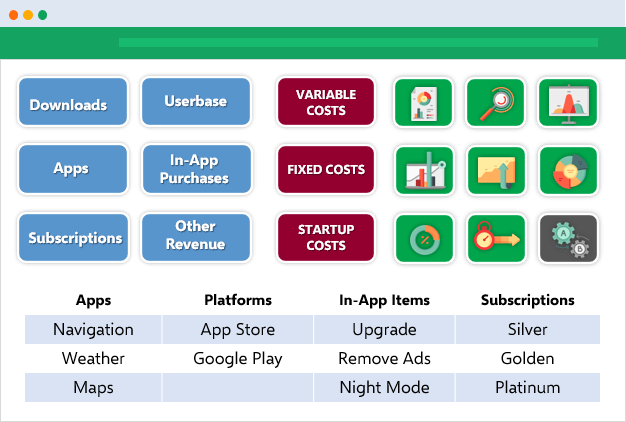
This is a comprehensive Feasibility Study Excel Template for app startups with download projections, costs, financial calculations, charts, dashboard, and more.
The business world is demanding. It is not enough just to make the calculations, set up your tables, and write the text. You have to create pie charts, trends, line graphs, and many more. Whether you are getting prepared for your pitch or make a presentation in your company, you can use Excel’s chart features.
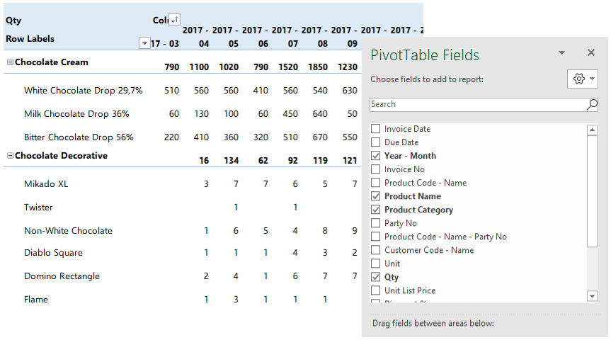
Pivot Tables
One of the greatest features which Excel offers is Pivot tables. This is an advanced Excel tool that helps you create dynamic summary reports from raw data very easily. After you create your table you can play with parameters easily with a drag and drop interface.
It looks like this:
Dashboards
Complex excel models do have lots of variables, calculations, and settings. And instead of managing all variables one by one on different sheets, different places it is a very good idea to put them together like a “control panel”.
You can think dashboards as cockpits of planes.
Recently dashboards became very popular. There are lots of training videos about how to build and design control panels for our excel models. Actually, they are not so different from the rest of the calculations.
But the main idea is: if there is something you may want to change, later on, don’t write it directly in the formula but bind it to a variable.
Let’s say you are building a sales report for your manager. He asks you to make the file changeable so that he can see the results in US dollars or Euros according to the situation. Instead of writing an Fx rate into the calculations, you should bind this to a cell that you can play with later on.
Like this:
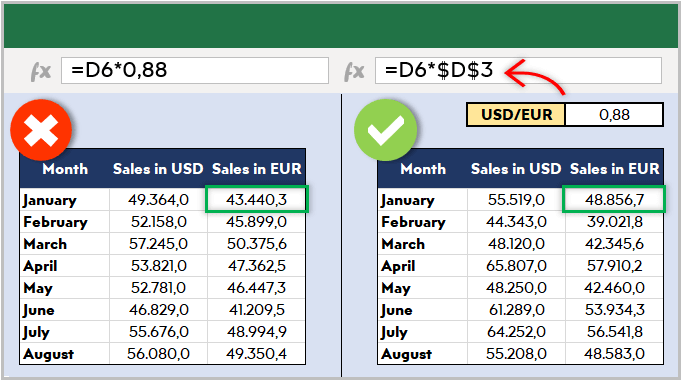
This may seem so obvious to some of you. But this is the basic approach of all dashboards in excel files. Of course, you can improve it with more complex formulas, buttons, cool charts, and even VBA but the main idea stands still.
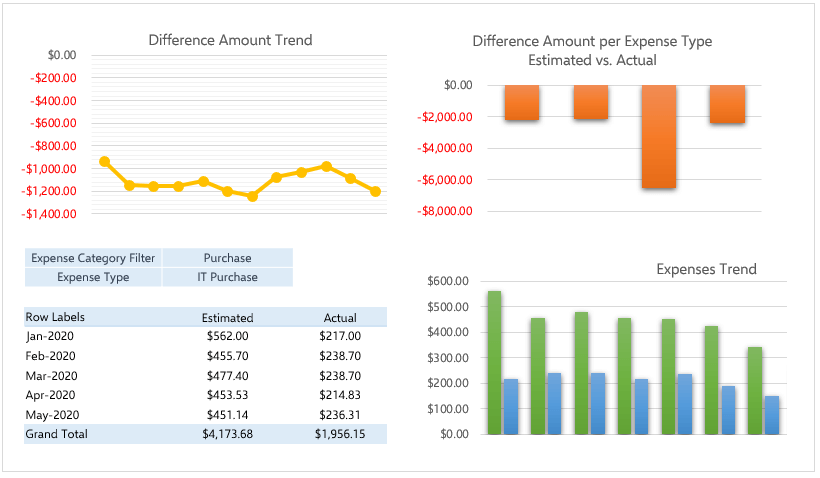
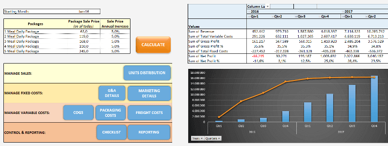
Here is an example of a complete set of the dashboard:
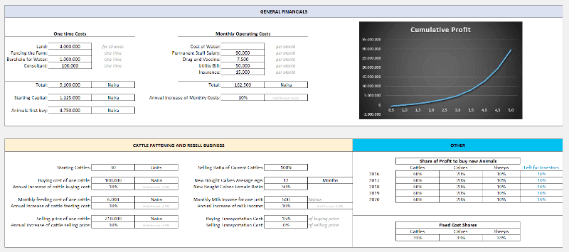
Or a dashboard for a livestock feasibility study:
If you are interested in Sales Dashboards, you may want to check out our Excel template:
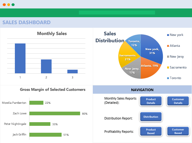
This is an interactive Sales Report Template in Excel. Features a dashboard with profitability, sales analysis and charts.
Other than that, Marketing ROI Calculator would be very helpful to prioritize your marketing campaigns in Excel:
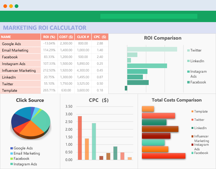
It will provide essential metrics and help you to manage all your marketing campaign channels in one place.
Most of the users who use Excel extensively are already coding. But if you ask them whether they know how to code most probably they will say no. Of course, writing formulas is a very small part of the things you can do with VBA. It is a strong programming language that lets you create small scripts (macros), user forms, user-defined functions, add-ins, and even games! (which we will touch below separately)
I will not dive into VBA here since it is a detailed area. But there are some basic things that will be beneficial to know for those who use Excel often:
- You can record macros for repeating jobs: You don’t need to code from scratch. Just click on the record macro button and it will write the code for you in the background. (If you want, you can modify later on)
- It extends the borders of Excel world. If you feel like you are limited somehow in Excel, you are more like an advanced user. It is time to get a little bit into VBA.
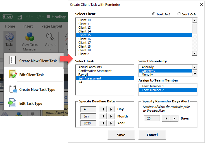
- You can create user forms with VBA only. If you see something like this, know that it is using VBA:
VBA is quite powerful and if you work with Excel extensively you won’t regret learning a bit. For example wouldn’t it be nice if you could send bulk emails from an Excel spreadsheat with a button click?
It is not surprising for spreadsheet software like Excel to offer advanced math techniques to make more complicated studies. (To be honest, I am not a statistics expert but with an engineering background, I will try to do my best to explain the basics. Feel free to correct me if I’m wrong)
Data analysis is a trending concept for recent years with the development of powerful computers and improved software. We are collecting and recording much much more data compared to the past. Take a look at this chart to understand what I mean:

Especially this part:
“more data has been created in the past two years than in the entire previous history of the human race”
It is a bit frightening, isn’t it? Ok, we are not going to dive into the “Big Data” world. Let’s get back to our humble excel world.
As we collect this much data, some people will want to analyze it. Otherwise, it makes no sense to spend billions of dollars on those data centers. Excel has built-in functions for basic descriptive statistics methods like Mean, Median, Mode, Standard Deviation, Variance etc.
But if we want to go a bit further I will mention two Excel features (actually add-ins) at this step: Solver and Regression Analysis
Solver
Have you ever heard of “optimization”? When we have more than one parameters that affect the outcome, we can only have a most optimized solution rather than a maximum solution. This may sound weird but it is very valid in our daily lives.
One of the simplest and popular examples is: Farmer Fence Optimization Problem
“A farmer owns 500 meters of the fence and wants to enclose the largest possible rectangular area. How should he use his fence?”
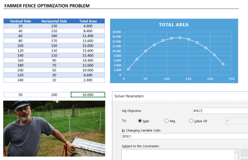
This is a very simple example to explain what a solver does. But actually, you can run much more complicated data sets with Solver.
Regression Analysis
Since this is a bit advanced topic for this blog post, I will only touch the surface.
In most simple terms, regression analysis helps you find the correlation between the variables. For example, you may want to know what is the relation between the number of birds flown over your head and the money you earned today. (sorry for the silly example. No, I am not curious about it  You will need to gather sample data and put in an analysis to see if there is any correlation.
It seems something like this:
You put your data:
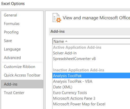
Run the regression from Analysis Toolpak:
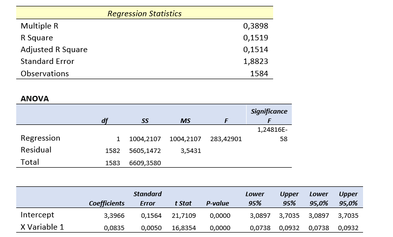
And get results something like this:
Of course, there is much more sophisticated software to run data analysis. However, there is a joke in business intelligence communities:
- What is the most used feature of any business intelligence solution?
- It is “Export to Excel”
Looks like we won’t stop using Excel anytime soon.
Coming back from boring data analysis world, let’s mention the simplest and most handy usage area of excel: Make Lists!
It is already self-explaining so I won’t bother with the details. When you want to list down some simple data, take notes, create to-do lists, or anything. Just open the excel and write it down. Did we mention that “paper alternative” thing? Oh yes, we did.
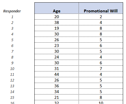
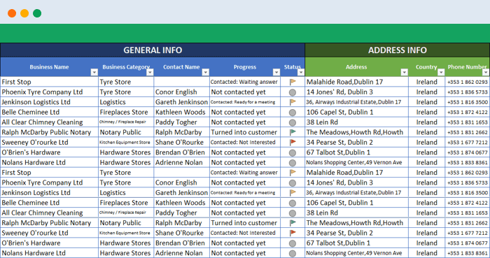
A lead list example:
You can also convert PDF files into Excel files in order to make it easier to work on. This can be done automatically with some software. But some pdf files cannot be processed automatically (like handwritten documents, scanned invoices, etc). You will need to do it manually.
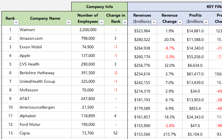
When you want to play with the data on a web page, you can easily copy-paste it into an excel file and then you can sort, filter or do anything you want:
For example, Fortune 500 US List:
Everybody loves to-do lists. And we have created useful to-do list in Excel for business or personal uses. Check it out, it is free:
To-Do List Excel Template
We already mentioned this in the VBA section above. But it is worth to talk a bit more.
Visual Basic allows you to code complex things like games as well. But of course, don’t expect a GTA or FIFA. Things like chess, sudoku, or Monopoly is OK. But, a few people have gone far and created more complicated things, like an RPG game. Take a look at this:
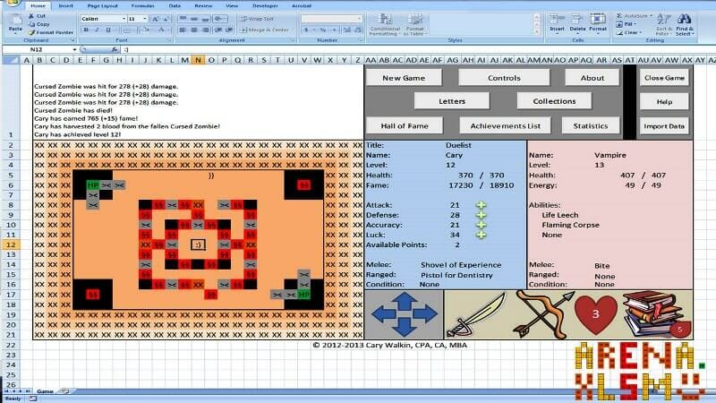
This game has been created by an accountant, Cary Walkin. I know it doesn’t look great but it is in Excel! (you can play it at the office  )
)
Another example:

A flight simulator in Excel?? Is it the same thing we use to sum up the sales figures? Lol yeah.
You can also embed flash games into Excel (like Super Mario, Angry Birds or whatever) But I count them off as they are not built with VBA.
As we mentioned in the Financial Modeling section, Excel is quite good for creating dynamic results according to the inputs. We get the benefit of this to create interactive tools.
One example that comes to my mind is this spreadsheet, guys from San Francisco have prepared:
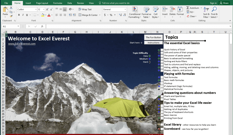
I haven’t tried it myself but an Excel tutorial in Excel. Liked the idea!
Another similar interactive Excel learning tool is from Keyskillset:
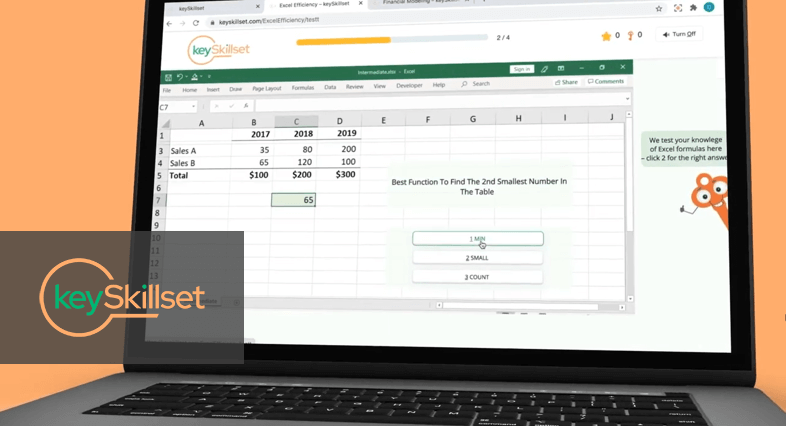
Actually, this is not completely in Excel and works as separate software but I liked how they combine the Excel training with gamification features.
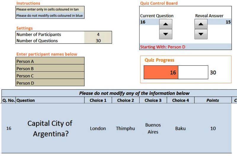
Quizzes are good tools for interactive learning and you can prepare in Excel as well. A quizmaster template from indzara.com:
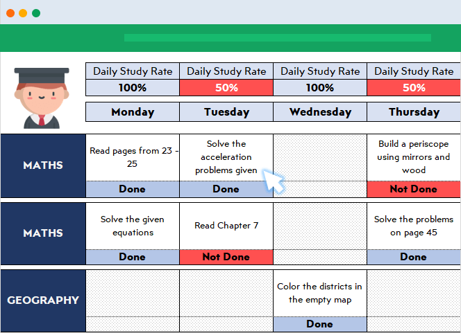
A student lesson plan template in excel which we have prepared recently:
You can learn Excel in Excel!
As said: Practice Makes Perfect!
You can test your Excel skills in Excel with Excel Formulas Trainer:
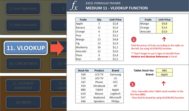
This is actually an Excel template prepared with VBA macros and basically works as a practice worksheet. It has 30 sections and around 100 questions. You can learn VLOOKUP, IF and much more excel formulas by doing. If you like the idea of “learning by doing”, then it is worth to check.
Also, this online course from GoSkills is for everyone as well, covering beginner, intermediate and advanced lessons.
By cheat sheets, we don’t refer to the piece of paper with information written down on it that an unethical person might create if they weren’t prepared for a test. What we mean is a reference tool that provides simple, brief instructions for accomplishing a specific task. We use this term because it is highly popular recently.
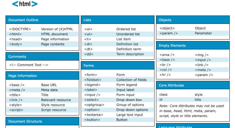
For example, this is a cheat sheet:
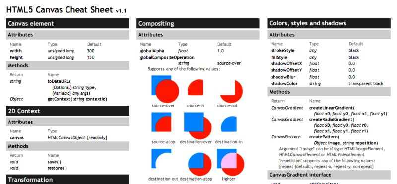
This compacted and summarized info is very useful in many aspects. When you try to memorize things, lookup, reference, etc. And can be easily created with Excel. Let’s make a Google search for a cheat sheet made in Excel.
This one is from Dave Child (cheatography.com) and I was also using this one I first learned HTML:
The last example is an Excel Cheatsheet made for Excel shortcuts:
Of course, if you are looking for stylish infographics and cheat sheets, you should check out design software.
I know Excel is maybe not the best tool to do these. There are great programs or websites to make mockups, diagrams, brainstorming, mind-mapping, or project scheduling. But there are habits as well. Even though I am very open to try and use these kinds of brand-new tools, I find myself using excel for a mockup or a mind map. (select shapes, put notes, put arrows, change colors etc. Omg it is tedious)
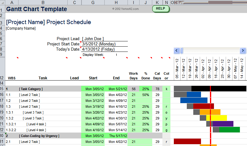
Gantt charts can be a bit old-school as agile project management methods are increasing in popularity, they are still being used widely. There are several Gantt chart excel templates on the web.
A Gantt chart example from vertex42.com:
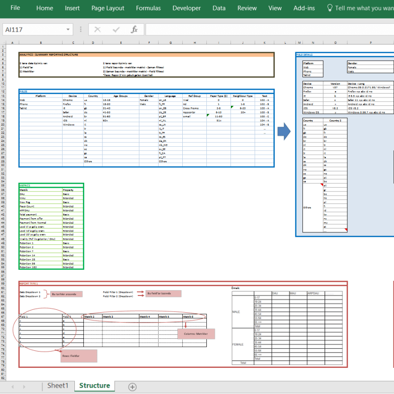
I just found out a reporting structure mockup I have prepared in Excel once upon a time:
By the way, did you see our Automatic Organization Chart Generator?
This is an Excel template that lets you create organization charts from Excel lists with a click of a button. It can be useful for small business owners and Human Resources departments.
These type of charts are directly related to Excel as most of the companies already keep their data in spreadsheets. But I also know people who even build their website mockups in Excel (with links to other sections, placement of buttons, sliders etc.).
Sometimes you may need your excel files to be updated automatically from a live data source. For example, if you are making a stock market analysis and want the latest data of some stock prices at NYSE, you can connect your Excel file to a data feed and let it take the latest info automatically (unless you want to input them one by one!)
As this is a comprehensive topic I will leave it for another post. But here is a few things you can fetch into excel:
- Stock prices
- Match results of soccer, NBA, NFL or any sports games (from live score sites)
- Fx rates
- Real-time flight data of airports
- Any info in a shared database (whether it is your company intranet or public)
This topic is getting more and more important as most data is kept on cloud systems. We don’t download info bits to our computers as we used to do in the past. So, Microsoft is working hard to improve the web integration of Excel.
Recommended Reading: Can Excel Extract Data From Website?
Yes, it is not the best idea to use Excel as a database. Because it is not designed for this purpose. Queries will take a long time especially when data gets bigger. It can be unreliable sometimes and not very secure. It is all accepted. However, we are not always after a complete set of the database systems and it can serve us as a mini-warehouse for our little data.

For example, if you keep records of your invoice data and want to make some sales analysis, it can be a good starting point. If later, you want to see more details, want to record more breakdowns you will need to move to a “real database”. It can be Access, SQL or anything. Just keep an eye on your Excel file because it has a maximum of 1 million rows.
Some of you may say “hey, it is more than enough, isn’t it?”
Generally yes. But you cannot believe how data increase in size when you want to see details. I remember when I was working as an analyst in a game development company, we were holding records of 1+ billion rows of data.
Precisely because of that, we have built some of our Excel templates (which is the favorite feature of all the users) with a database section. You may check our Invoice Generators and see how invoice recording would be super easy in Excel!
Conclusion
As the internet gets more available for everybody people started to use collaboration platforms more than before. In this aspect, online spreadsheet applications, like Google Sheets, increase in popularity and stands as a competitor to Microsoft’s Excel. Other free alternatives like open office or libre office are also popular. But if you need the advanced functionalities of Excel there is still no substitute.

Microsoft is improving the software actively. PowerPivot, Power BI, and Excel Online are all brand new features they developed recently. We will wait and see how things evolve in the following years. (investintech.com has made interviews with Excel experts about the future of Excel)
I tried to cover most of the things that can be done with Excel. If I have missed anything or if you find any errors, let me know by commenting down or sending an email.
Also, don’t forget to check our Excel Templates Collection. You may find something useful for yourself:
Excel Templates and Spreadsheets – Someka
Complete List of Things You Can Do With Excel
- Tools, Calculators and Simulations.
- Dashboards and Reports with Charts.
- Automate Jobs with VBA macros.
- Solver Add-in & Statistical Analysis.
- Data Entry and Lists.
- Games in Excel!
- Educational use with Interactive features.
- Create Cheatsheets with Excel.
Contents
- 1 What are 7 things you can use Excel for?
- 2 What are the 10 uses of Microsoft Excel?
- 3 What are the 3 common uses for Excel?
- 4 What can Excel be used for at home?
- 5 What are the five uses of spreadsheet?
- 6 How can excel help you as a student?
- 7 How excel is useful in our life?
- 8 Is Excel a good skill?
- 9 What are 3 uses of spreadsheets?
- 10 How are spreadsheets useful for users?
- 11 What are the Excel features?
- 12 How do I make Excel fun?
- 13 How can excel functions help in future career?
- 14 Is Excel worth learning in 2021?
- 15 Is Excel still relevant 2021?
- 16 What are the basic things to learn in Excel?
- 17 What can I make a spreadsheet of?
- 18 How do I make an Excel spreadsheet look pretty?
- 19 How do you use a spreadsheet as a planner?
- 20 What’s a worksheet in Excel?
What are 7 things you can use Excel for?
More Than a Spreadsheet: 7 Things You Can Do with Microsoft Excel
- Accounting. Excel has long been a trusted accounting tool.
- Data Entry, Storage, and Verification. At its core, Excel is data-entry software.
- Data Visualisation.
- Data Forecasting.
- Inventory Tracking.
- Project Management.
- Creating Forms.
What are the 10 uses of Microsoft Excel?
Top 10 Uses of Microsoft Excel in Business
- Business Analysis. The number 1 use of MS Excel in the workplace is to do business analysis.
- People Management.
- Managing Operations.
- Performance Reporting.
- Office Administration.
- Strategic Analysis.
- Project Management.
- Managing Programs.
What are the 3 common uses for Excel?
The main uses of Excel include:
- Data entry.
- Data management.
- Accounting.
- Financial analysis.
- Charting and graphing.
- Programming.
- Time management.
- Task management.
What can Excel be used for at home?
You can use Excel to store, organize, and analyze data. Excel is Microsoft’s spreadsheet program, a part of the Microsoft 365 suite of products. Here’s a crash course in the basics of using Microsoft Excel.
What are the five uses of spreadsheet?
What Is the Purpose of Using a Spreadsheet?
- Business Data Storage. A spreadsheet is an easy way to store all different kinds of data.
- Accounting and Calculation Uses.
- Budgeting and Spending Help.
- Assisting with Data Exports.
- Data Sifting and Cleanup.
- Generating Reports and Charts.
- Business Administrative Tasks.
How can excel help you as a student?
Excel reduces the difficulty of plotting data and allows students a means for interpreting the data. You can also reverse the traditional process of analyzing data by giving students a completed chart and see if they can reconstruct the underlying worksheet.
How excel is useful in our life?
Excel helps you in career management, time management, learning management, life management, and so on. If you are a student, then you can manage all your expenses with the help of excel.
Is Excel a good skill?
It contains a spreadsheet that can automatically input, calculate and analyze data, which makes it a valuable skill for the workplace. Employees can use Excel to accomplish an abundance of daily tasks.
What are 3 uses of spreadsheets?
The three most common general uses for spreadsheet software are to create budgets, produce graphs and charts, and for storing and sorting data. Within business spreadsheet software is used to forecast future performance, calculate tax, completing basic payroll, producing charts and calculating revenues.
How are spreadsheets useful for users?
A spreadsheet is a tool that is used to store, manipulate and analyze data.These programs allow users to work with data in a variety of ways to create budgets, forecasts, inventories, schedules, charts, graphs and many other data based worksheets.
What are the Excel features?
Features of Microsoft Excel
- Add Header and Footer. MS Excel allows us to keep the header and footer in our spreadsheet document.
- Find and Replace Command.
- Password Protection.
- Data Filtering.
- Data Sorting.
- Built-in formulae.
- Create different charts (Pivot Table Report)
- Automatically edits the result.
How do I make Excel fun?
Excel can be Exciting – 15 fun things you can do with your spreadsheet in less than 5 seconds
- Change the shape / color of cell comments.
- Filter unique items from a list.
- Sort from Left to Right.
- Hide the grid lines from your sheets.
- Add rounded border to your charts, make them look smooth.
How can excel functions help in future career?
Benefits of Excel for Employees
- Sharpening Your Skill Set.
- Improving Your Efficiency and Productivity.
- Making Yourself a More Valuable Member of the Company.
- Making You Better at Organizing Data.
- It Can Make Your Job Easier.
- It Creates Greater Efficiency and Heightens Productivity.
Is Excel worth learning in 2021?
Q: Is VBA still relevant in 2021? Excel is a program that is still worked with a lot by many companies/people, so it is still relevant to learn VBA in 2021.
Is Excel still relevant 2021?
In the age of data analysis, Microsoft Excel is still necessary.One such program, which often goes unnoticed when it comes to the analysis of data, is Microsoft Excel. Microsoft excel is still relevant in the age of data analysis and advanced technologies.
What are the basic things to learn in Excel?
Basic Skills for Excel Users
- Sum or Count cells, based on one criterion or multiple criteria.
- Build a Pivot Table to summarize date.
- Write a formula with absolute and relative references.
- Create a drop down list of options in a cell, for easier data entry.
- Sort a list of text and/or numbers without messing up the data.
What can I make a spreadsheet of?
10 Amazingly Useful Spreadsheet Templates to Organize Your Life
- Excel Money Management Template.
- To-Do List.
- Medication List.
- Travel Budget Worksheet.
- Checkbook Register.
- Home Inventory Checklist.
- Meal Planner.
- Project Schedule Template.
How do I make an Excel spreadsheet look pretty?
Excel for Architects – 9 Steps to Beautiful Spreadsheets
- Choose a good font.
- Align your data.
- Give your data some space.
- Define your headers.
- Choose your colors carefully.
- Shade alternate rows for readability.
- Use Grids Sparingly.
- Create cell styles for consistency.
How do you use a spreadsheet as a planner?
Here’s how to set up your weekly planner using Google Sheets.
- Step 1: Go to spreadsheets.google.com and click “Template Gallery” to see all available templates.
- Step 2: Choose “Schedule” template.
- Step 3: Set the starting date in cell C2.
- Step 1: Make yourself a copy of this spreadsheet:
What’s a worksheet in Excel?
The term Worksheet used in Excel documents is a collection of cells organized in rows and columns. It is the working surface you interact with to enter data. Each worksheet contains 1048576 rows and 16384 columns and serves as a giant table that allows you to organize information.
Sometimes, Excel seems too good to be true. All I have to do is enter a formula, and pretty much anything I’d ever need to do manually can be done automatically.
Need to merge two sheets with similar data? Excel can do it.
Need to do simple math? Excel can do it.
Need to combine information in multiple cells? Excel can do it.
In this post, I’ll go over the best tips, tricks, and shortcuts you can use right now to take your Excel game to the next level. No advanced Excel knowledge required.
![Download 10 Excel Templates for Marketers [Free Kit]](https://no-cache.hubspot.com/cta/default/53/9ff7a4fe-5293-496c-acca-566bc6e73f42.png)
-
What is Excel?
-
Excel Basics
-
How to Use Excel
-
Excel Tips
-
Excel Keyboard Shortcuts
What is Excel?
Microsoft Excel is powerful data visualization and analysis software, which uses spreadsheets to store, organize, and track data sets with formulas and functions. Excel is used by marketers, accountants, data analysts, and other professionals. It’s part of the Microsoft Office suite of products. Alternatives include Google Sheets and Numbers.
Find more Excel alternatives here.
What is Excel used for?
Excel is used to store, analyze, and report on large amounts of data. It is often used by accounting teams for financial analysis, but can be used by any professional to manage long and unwieldy datasets. Examples of Excel applications include balance sheets, budgets, or editorial calendars.
Excel is primarily used for creating financial documents because of its strong computational powers. You’ll often find the software in accounting offices and teams because it allows accountants to automatically see sums, averages, and totals. With Excel, they can easily make sense of their business’ data.
While Excel is primarily known as an accounting tool, professionals in any field can use its features and formulas — especially marketers — because it can be used for tracking any type of data. It removes the need to spend hours and hours counting cells or copying and pasting performance numbers. Excel typically has a shortcut or quick fix that speeds up the process.
You can also download Excel templates below for all of your marketing needs.
After you download the templates, it’s time to start using the software. Let’s cover the basics first.
Excel Basics
If you’re just starting out with Excel, there are a few basic commands that we suggest you become familiar with. These are things like:
- Creating a new spreadsheet from scratch.
- Executing basic computations like adding, subtracting, multiplying, and dividing.
- Writing and formatting column text and titles.
- Using Excel’s auto-fill features.
- Adding or deleting single columns, rows, and spreadsheets. (Below, we’ll get into how to add things like multiple columns and rows.)
- Keeping column and row titles visible as you scroll past them in a spreadsheet, so that you know what data you’re filling as you move further down the document.
- Sorting your data in alphabetical order.
Let’s explore a few of these more in-depth.
For instance, why does auto-fill matter?
If you have any basic Excel knowledge, it’s likely you already know this quick trick. But to cover our bases, allow me to show you the glory of autofill. This lets you quickly fill adjacent cells with several types of data, including values, series, and formulas.
There are multiple ways to deploy this feature, but the fill handle is among the easiest. Select the cells you want to be the source, locate the fill handle in the lower-right corner of the cell, and either drag the fill handle to cover cells you want to fill or just double click:
 Similarly, sorting is an important feature you’ll want to know when organizing your data in Excel.
Sometimes you may have a list of data that has no organization whatsoever. Maybe you exported a list of your marketing contacts or blog posts. Whatever the case may be, Excel’s sort feature will help you alphabetize any list.
Click on the data in the column you want to sort. Then click on the «Data» tab in your toolbar and look for the «Sort» option on the left. If the «A» is on top of the «Z,» you can just click on that button once. If the «Z» is on top of the «A,» click on the button twice. When the «A» is on top of the «Z,» that means your list will be sorted in alphabetical order. However, when the «Z» is on top of the «A,» that means your list will be sorted in reverse alphabetical order.
Let’s explore more of the basics of Excel (along with advanced features) next.
To use Excel, you only need to input the data into the rows and columns. And then you’ll use formulas and functions to turn that data into insights.
We’re going to go over the best formulas and functions you need to know. But first, let’s take a look at the types of documents you can create using the software. That way, you have an overarching understanding of how you can use Excel in your day-to-day.
Documents You Can Create in Excel
Not sure how you can actually use Excel in your team? Here is a list of documents you can create:
- Income Statements: You can use an Excel spreadsheet to track a company’s sales activity and financial health.
- Balance Sheets: Balance sheets are among the most common types of documents you can create with Excel. It allows you to get a holistic view of a company’s financial standing.
- Calendar: You can easily create a spreadsheet monthly calendar to track events or other date-sensitive information.
Here are some documents you can create specifically for marketers.
- Marketing Budgets: Excel is a strong budget-keeping tool. You can create and track marketing budgets, as well as spend, using Excel. If you don’t want to create a document from scratch, download our marketing budget templates for free.
- Marketing Reports: If you don’t use a marketing tool such as Marketing Hub, you might find yourself in need of a dashboard with all of your reports. Excel is an excellent tool to create marketing reports. Download free Excel marketing reporting templates here.
- Editorial Calendars: You can create editorial calendars in Excel. The tab format makes it extremely easy to track your content creation efforts for custom time ranges. Download a free editorial content calendar template here.
- Traffic and Leads Calculator: Because of its strong computational powers, Excel is an excellent tool to create all sorts of calculators — including one for tracking leads and traffic. Click here to download a free premade lead goal calculator.
This is only a small sampling of the types of marketing and business documents you can create in Excel. We’ve created an extensive list of Excel templates you can use right now for marketing, invoicing, project management, budgeting, and more.
In the spirit of working more efficiently and avoiding tedious, manual work, here are a few Excel formulas and functions you’ll need to know.
Excel Formulas
It’s easy to get overwhelmed by the wide range of Excel formulas that you can use to make sense out of your data. If you’re just getting started using Excel, you can rely on the following formulas to carry out some complex functions — without adding to the complexity of your learning path.
- Equal sign: Before creating any formula, you’ll need to write an equal sign (=) in the cell where you want the result to appear.
- Addition: To add the values of two or more cells, use the + sign. Example: =C5+D3.
- Subtraction: To subtract the values of two or more cells, use the — sign. Example: =C5-D3.
- Multiplication: To multiply the values of two or more cells, use the * sign. Example: =C5*D3.
- Division: To divide the values of two or more cells, use the / sign. Example: =C5/D3.
Putting all of these together, you can create a formula that adds, subtracts, multiplies, and divides all in one cell. Example: =(C5-D3)/((A5+B6)*3).
For more complex formulas, you’ll need to use parentheses around the expressions to avoid accidentally using the PEMDAS order of operations. Keep in mind that you can use plain numbers in your formulas.
Excel Functions
Excel functions automate some of the tasks you would use in a typical formula. For instance, instead of using the + sign to add up a range of cells, you’d use the SUM function. Let’s look at a few more functions that will help automate calculations and tasks.
- SUM: The SUM function automatically adds up a range of cells or numbers. To complete a sum, you would input the starting cell and the final cell with a colon in between. Here’s what that looks like: SUM(Cell1:Cell2). Example: =SUM(C5:C30).
- AVERAGE: The AVERAGE function averages out the values of a range of cells. The syntax is the same as the SUM function: AVERAGE(Cell1:Cell2). Example: =AVERAGE(C5:C30).
- IF: The IF function allows you to return values based on a logical test. The syntax is as follows: IF(logical_test, value_if_true, [value_if_false]). Example: =IF(A2>B2,»Over Budget»,»OK»).
- VLOOKUP: The VLOOKUP function helps you search for anything on your sheet’s rows. The syntax is: VLOOKUP(lookup value, table array, column number, Approximate match (TRUE) or Exact match (FALSE)). Example: =VLOOKUP([@Attorney],tbl_Attorneys,4,FALSE).
- INDEX: The INDEX function returns a value from within a range. The syntax is as follows: INDEX(array, row_num, [column_num]).
- MATCH: The MATCH function looks for a certain item in a range of cells and returns the position of that item. It can be used in tandem with the INDEX function. The syntax is: MATCH(lookup_value, lookup_array, [match_type]).
- COUNTIF: The COUNTIF function returns the number of cells that meet a certain criteria or have a certain value. The syntax is: COUNTIF(range, criteria). Example: =COUNTIF(A2:A5,»London»).
Okay, ready to get into the nitty-gritty? Let’s get to it. (And to all the Harry Potter fans out there … you’re welcome in advance.)
Excel Tips
- Use Pivot tables to recognize and make sense of data.
- Add more than one row or column.
- Use filters to simplify your data.
- Remove duplicate data points or sets.
- Transpose rows into columns.
- Split up text information between columns.
- Use these formulas for simple calculations.
- Get the average of numbers in your cells.
- Use conditional formatting to make cells automatically change color based on data.
- Use IF Excel formula to automate certain Excel functions.
- Use dollar signs to keep one cell’s formula the same regardless of where it moves.
- Use the VLOOKUP function to pull data from one area of a sheet to another.
- Use INDEX and MATCH formulas to pull data from horizontal columns.
- Use the COUNTIF function to make Excel count words or numbers in any range of cells.
- Combine cells using ampersand.
- Add checkboxes.
- Hyperlink a cell to a website.
- Add drop-down menus.
- Use the format painter.
Note: The GIFs and visuals are from a previous version of Excel. When applicable, the copy has been updated to provide instruction for users of both newer and older Excel versions.
1. Use Pivot tables to recognize and make sense of data.
Pivot tables are used to reorganize data in a spreadsheet. They won’t change the data that you have, but they can sum up values and compare different information in your spreadsheet, depending on what you’d like them to do.
Let’s take a look at an example. Let’s say I want to take a look at how many people are in each house at Hogwarts. You may be thinking that I don’t have too much data, but for longer data sets, this will come in handy.
To create the Pivot Table, I go to Data > Pivot Table. If you’re using the most recent version of Excel, you’d go to Insert > Pivot Table. Excel will automatically populate your Pivot Table, but you can always change around the order of the data. Then, you have four options to choose from.
- Report Filter: This allows you to only look at certain rows in your dataset. For example, if I wanted to create a filter by house, I could choose to only include students in Gryffindor instead of all students.
- Column Labels: These would be your headers in the dataset.
- Row Labels: These could be your rows in the dataset. Both Row and Column labels can contain data from your columns (e.g. First Name can be dragged to either the Row or Column label — it just depends on how you want to see the data.)
- Value: This section allows you to look at your data differently. Instead of just pulling in any numeric value, you can sum, count, average, max, min, count numbers, or do a few other manipulations with your data. In fact, by default, when you drag a field to Value, it always does a count.
Since I want to count the number of students in each house, I’ll go to the Pivot table builder and drag the House column to both the Row Labels and the Values. This will sum up the number of students associated with each house.
2. Add more than one row or column.
As you play around with your data, you might find you’re constantly needing to add more rows and columns. Sometimes, you may even need to add hundreds of rows. Doing this one-by-one would be super tedious. Luckily, there’s always an easier way.
To add multiple rows or columns in a spreadsheet, highlight the same number of preexisting rows or columns that you want to add. Then, right-click and select «Insert.»
In the example below, I want to add an additional three rows. By highlighting three rows and then clicking insert, I’m able to add an additional three blank rows into my spreadsheet quickly and easily.
3. Use filters to simplify your data.
When you’re looking at very large data sets, you don’t usually need to be looking at every single row at the same time. Sometimes, you only want to look at data that fit into certain criteria.
That’s where filters come in.
Filters allow you to pare down your data to only look at certain rows at one time. In Excel, a filter can be added to each column in your data — and from there, you can then choose which cells you want to view at once.
Let’s take a look at the example below. Add a filter by clicking the Data tab and selecting «Filter.» Clicking the arrow next to the column headers and you’ll be able to choose whether you want your data to be organized in ascending or descending order, as well as which specific rows you want to show.
In my Harry Potter example, let’s say I only want to see the students in Gryffindor. By selecting the Gryffindor filter, the other rows disappear.
 Pro Tip: Copy and paste the values in the spreadsheet when a Filter is on to do additional analysis in another spreadsheet.
4. Remove duplicate data points or sets.
Larger data sets tend to have duplicate content. You may have a list of multiple contacts in a company and only want to see the number of companies you have. In situations like this, removing the duplicates comes in quite handy.
To remove your duplicates, highlight the row or column that you want to remove duplicates of. Then, go to the Data tab and select «Remove Duplicates» (which is under the Tools subheader in the older version of Excel). A pop-up will appear to confirm which data you want to work with. Select «Remove Duplicates,» and you’re good to go.
You can also use this feature to remove an entire row based on a duplicate column value. So if you have three rows with Harry Potter’s information and you only need to see one, then you can select the whole dataset and then remove duplicates based on email. Your resulting list will have only unique names without any duplicates.
5. Transpose rows into columns.
When you have rows of data in your spreadsheet, you might decide you actually want to transform the items in one of those rows into columns (or vice versa). It would take a lot of time to copy and paste each individual header — but what the transpose feature allows you to do is simply move your row data into columns, or the other way around.
Start by highlighting the column that you want to transpose into rows. Right-click it, and then select «Copy.» Next, select the cells on your spreadsheet where you want your first row or column to begin. Right-click on the cell, and then select «Paste Special.» A module will appear — at the bottom, you’ll see an option to transpose. Check that box and select OK. Your column will now be transferred to a row or vice-versa.
On newer versions of Excel, a drop-down will appear instead of a pop-up.

6. Split up text information between columns.
What if you want to split out information that’s in one cell into two different cells? For example, maybe you want to pull out someone’s company name through their email address. Or perhaps you want to separate someone’s full name into a first and last name for your email marketing templates.
Thanks to Excel, both are possible. First, highlight the column that you want to split up. Next, go to the Data tab and select «Text to Columns.» A module will appear with additional information.
First, you need to select either «Delimited» or «Fixed Width.»
- «Delimited» means you want to break up the column based on characters such as commas, spaces, or tabs.
- «Fixed Width» means you want to select the exact location on all the columns that you want the split to occur.
In the example case below, let’s select «Delimited» so we can separate the full name into first name and last name.
Then, it’s time to choose the Delimiters. This could be a tab, semi-colon, comma, space, or something else. («Something else» could be the «@» sign used in an email address, for example.) In our example, let’s choose the space. Excel will then show you a preview of what your new columns will look like.
When you’re happy with the preview, press «Next.» This page will allow you to select Advanced Formats if you choose to. When you’re done, click «Finish.»
7. Use formulas for simple calculations.
In addition to doing pretty complex calculations, Excel can help you do simple arithmetic like adding, subtracting, multiplying, or dividing any of your data.
- To add, use the + sign.
- To subtract, use the — sign.
- To multiply, use the * sign.
- To divide, use the / sign.
You can also use parentheses to ensure certain calculations are done first. In the example below (10+10*10), the second and third 10 were multiplied together before adding the additional 10. However, if we made it (10+10)*10, the first and second 10 would be added together first.
8. Get the average of numbers in your cells.
If you want the average of a set of numbers, you can use the formula =AVERAGE(Cell1:Cell2). If you want to sum up a column of numbers, you can use the formula =SUM(Cell1:Cell2).
9. Use conditional formatting to make cells automatically change color based on data.
Conditional formatting allows you to change a cell’s color based on the information within the cell. For example, if you want to flag certain numbers that are above average or in the top 10% of the data in your spreadsheet, you can do that. If you want to color code commonalities between different rows in Excel, you can do that. This will help you quickly see information that is important to you.
To get started, highlight the group of cells you want to use conditional formatting on. Then, choose «Conditional Formatting» from the Home menu and select your logic from the dropdown. (You can also create your own rule if you want something different.) A window will pop up that prompts you to provide more information about your formatting rule. Select «OK» when you’re done, and you should see your results automatically appear.
10. Use the IF Excel formula to automate certain Excel functions.
Sometimes, we don’t want to count the number of times a value appears. Instead, we want to input different information into a cell if there is a corresponding cell with that information.
For example, in the situation below, I want to award ten points to everyone who belongs in the Gryffindor house. Instead of manually typing in 10’s next to each Gryffindor student’s name, I can use the IF Excel formula to say that if the student is in Gryffindor, then they should get ten points.
The formula is: IF(logical_test, value_if_true, [value_if_false])
Example Shown Below: =IF(D2=»Gryffindor»,»10″,»0″)
In general terms, the formula would be IF(Logical Test, value of true, value of false). Let’s dig into each of these variables.
- Logical_Test: The logical test is the «IF» part of the statement. In this case, the logic is D2=»Gryffindor» because we want to make sure that the cell corresponding with the student says «Gryffindor.» Make sure to put Gryffindor in quotation marks here.
- Value_if_True: This is what we want the cell to show if the value is true. In this case, we want the cell to show «10» to indicate that the student was awarded the 10 points. Only use quotation marks if you want the result to be text instead of a number.
- Value_if_False: This is what we want the cell to show if the value is false. In this case, for any student not in Gryffindor, we want the cell to show «0». Only use quotation marks if you want the result to be text instead of a number.
Note: In the example above, I awarded 10 points to everyone in Gryffindor. If I later wanted to sum the total number of points, I wouldn’t be able to because the 10’s are in quotes, thus making them text and not a number that Excel can sum.
The real power of the IF function comes when you string multiple IF statements together, or nest them. This allows you to set multiple conditions, get more specific results, and ultimately organize your data into more manageable chunks.
Ranges are one way to segment your data for better analysis. For example, you can categorize data into values that are less than 10, 11 to 50, or 51 to 100. Here’s how that looks in practice:
=IF(B3<11,“10 or less”,IF(B3<51,“11 to 50”,IF(B3<100,“51 to 100”)))
It can take some trial-and-error, but once you have the hang of it, IF formulas will become your new Excel best friend.
11. Use dollar signs to keep one cell’s formula the same regardless of where it moves.
Have you ever seen a dollar sign in an Excel formula? When used in a formula, it isn’t representing an American dollar; instead, it makes sure that the exact column and row are held the same even if you copy the same formula in adjacent rows.
You see, a cell reference — when you refer to cell A5 from cell C5, for example — is relative by default. In that case, you’re actually referring to a cell that’s five columns to the left (C minus A) and in the same row (5). This is called a relative formula. When you copy a relative formula from one cell to another, it’ll adjust the values in the formula based on where it’s moved. But sometimes, we want those values to stay the same no matter whether they’re moved around or not — and we can do that by turning the formula into an absolute formula.
To change the relative formula (=A5+C5) into an absolute formula, we’d precede the row and column values by dollar signs, like this: (=$A$5+$C$5). (Learn more on Microsoft Office’s support page here.)
12. Use the VLOOKUP function to pull data from one area of a sheet to another.
Have you ever had two sets of data on two different spreadsheets that you want to combine into a single spreadsheet?
For example, you might have a list of people’s names next to their email addresses in one spreadsheet, and a list of those same people’s email addresses next to their company names in the other — but you want the names, email addresses, and company names of those people to appear in one place.
I have to combine data sets like this a lot — and when I do, the VLOOKUP is my go-to formula.
Before you use the formula, though, be absolutely sure that you have at least one column that appears identically in both places. Scour your data sets to make sure the column of data you’re using to combine your information is exactly the same, including no extra spaces.
The formula: =VLOOKUP(lookup value, table array, column number, Approximate match (TRUE) or Exact match (FALSE))
The formula with variables from our example below: =VLOOKUP(C2,Sheet2!A:B,2,FALSE)
In this formula, there are several variables. The following is true when you want to combine information in Sheet 1 and Sheet 2 onto Sheet 1.
- Lookup Value: This is the identical value you have in both spreadsheets. Choose the first value in your first spreadsheet. In the example that follows, this means the first email address on the list, or cell 2 (C2).
- Table Array: The table array is the range of columns on Sheet 2 you’re going to pull your data from, including the column of data identical to your lookup value (in our example, email addresses) in Sheet 1 as well as the column of data you’re trying to copy to Sheet 1. In our example, this is «Sheet2!A:B.» «A» means Column A in Sheet 2, which is the column in Sheet 2 where the data identical to our lookup value (email) in Sheet 1 is listed. The «B» means Column B, which contains the information that’s only available in Sheet 2 that you want to translate to Sheet 1.
- Column Number: This tells Excel which column the new data you want to copy to Sheet 1 is located in. In our example, this would be the column that «House» is located in. «House» is the second column in our range of columns (table array), so our column number is 2. [Note: Your range can be more than two columns. For example, if there are three columns on Sheet 2 — Email, Age, and House — and you still want to bring House onto Sheet 1, you can still use a VLOOKUP. You just need to change the «2» to a «3» so it pulls back the value in the third column: =VLOOKUP(C2:Sheet2!A:C,3,false).]
- Approximate Match (TRUE) or Exact Match (FALSE): Use FALSE to ensure you pull in only exact value matches. If you use TRUE, the function will pull in approximate matches.
In the example below, Sheet 1 and Sheet 2 contain lists describing different information about the same people, and the common thread between the two is their email addresses. Let’s say we want to combine both datasets so that all the house information from Sheet 2 translates over to Sheet 1.
So when we type in the formula =VLOOKUP(C2,Sheet2!A:B,2,FALSE), we bring all the house data into Sheet 1.
Keep in mind that VLOOKUP will only pull back values from the second sheet that are to the right of the column containing your identical data. This can lead to some limitations, which is why some people prefer to use the INDEX and MATCH functions instead.
13. Use INDEX and MATCH formulas to pull data from horizontal columns.
Like VLOOKUP, the INDEX and MATCH functions pull in data from another dataset into one central location. Here are the main differences:
- VLOOKUP is a much simpler formula. If you’re working with large data sets that would require thousands of lookups, using the INDEX and MATCH function will significantly decrease load time in Excel.
- The INDEX and MATCH formulas work right-to-left, whereas VLOOKUP formulas only work as a left-to-right lookup. In other words, if you need to do a lookup that has a lookup column to the right of the results column, then you’d have to rearrange those columns in order to do a VLOOKUP. This can be tedious with large datasets and/or lead to errors.
So if I want to combine information in Sheet 1 and Sheet 2 onto Sheet 1, but the column values in Sheets 1 and 2 aren’t the same, then to do a VLOOKUP, I would need to switch around my columns. In this case, I’d choose to do an INDEX and MATCH instead.
Let’s look at an example. Let’s say Sheet 1 contains a list of people’s names and their Hogwarts email addresses, and Sheet 2 contains a list of people’s email addresses and the Patronus that each student has. (For the non-Harry Potter fans out there, every witch or wizard has an animal guardian called a «Patronus» associated with him or her.) The information that lives in both sheets is the column containing email addresses, but this email address column is in different column numbers on each sheet. I’d use the INDEX and MATCH formulas instead of VLOOKUP so I wouldn’t have to switch any columns around.
So what’s the formula, then? The formula is actually the MATCH formula nested inside the INDEX formula. You’ll see I differentiated the MATCH formula using a different color here.
The formula: =INDEX(table array, MATCH formula)
This becomes: =INDEX(table array, MATCH (lookup_value, lookup_array))
The formula with variables from our example below: =INDEX(Sheet2!A:A,(MATCH(Sheet1!C:C,Sheet2!C:C,0)))
Here are the variables:
- Table Array: The range of columns on Sheet 2 containing the new data you want to bring over to Sheet 1. In our example, «A» means Column A, which contains the «Patronus» information for each person.
- Lookup Value: This is the column in Sheet 1 that contains identical values in both spreadsheets. In the example that follows, this means the «email» column on Sheet 1, which is Column C. So: Sheet1!C:C.
- Lookup Array: This is the column in Sheet 2 that contains identical values in both spreadsheets. In the example that follows, this refers to the «email» column on Sheet 2, which happens to also be Column C. So: Sheet2!C:C.
Once you have your variables straight, type in the INDEX and MATCH formulas in the top-most cell of the blank Patronus column on Sheet 1, where you want the combined information to live.
14. Use the COUNTIF function to make Excel count words or numbers in any range of cells.
Instead of manually counting how often a certain value or number appears, let Excel do the work for you. With the COUNTIF function, Excel can count the number of times a word or number appears in any range of cells.
For example, let’s say I want to count the number of times the word «Gryffindor» appears in my data set.
The formula: =COUNTIF(range, criteria)
The formula with variables from our example below: =COUNTIF(D:D,»Gryffindor»)
In this formula, there are several variables:
- Range: The range that we want the formula to cover. In this case, since we’re only focusing on one column, we use «D:D» to indicate that the first and last column are both D. If I were looking at columns C and D, I would use «C:D.»
- Criteria: Whatever number or piece of text you want Excel to count. Only use quotation marks if you want the result to be text instead of a number. In our example, the criteria is «Gryffindor.»
Simply typing in the COUNTIF formula in any cell and pressing «Enter» will show me how many times the word «Gryffindor» appears in the dataset.
15. Combine cells using &.
Databases tend to split out data to make it as exact as possible. For example, instead of having a column that shows a person’s full name, a database might have the data as a first name and then a last name in separate columns. Or, it may have a person’s location separated by city, state, and zip code. In Excel, you can combine cells with different data into one cell by using the «&» sign in your function.
The formula with variables from our example below: =A2&» «&B2
Let’s go through the formula together using an example. Pretend we want to combine first names and last names into full names in a single column. To do this, we’d first put our cursor in the blank cell where we want the full name to appear. Next, we’d highlight one cell that contains a first name, type in an «&» sign, and then highlight a cell with the corresponding last name.
But you’re not finished — if all you type in is =A2&B2, then there will not be a space between the person’s first name and last name. To add that necessary space, use the function =A2&» «&B2. The quotation marks around the space tell Excel to put a space in between the first and last name.
To make this true for multiple rows, simply drag the corner of that first cell downward as shown in the example.
16. Add checkboxes.
If you’re using an Excel sheet to track customer data and want to oversee something that isn’t quantifiable, you could insert checkboxes into a column.
For example, if you’re using an Excel sheet to manage your sales prospects and want to track whether you called them in the last quarter, you could have a «Called this quarter?» column and check off the cells in it when you’ve called the respective client.
Here’s how to do it.
Highlight a cell you’d like to add checkboxes to in your spreadsheet. Then, click DEVELOPER. Then, under FORM CONTROLS, click the checkbox or the selection circle highlighted in the image below.
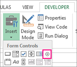
Once the box appears in the cell, copy it, highlight the cells you also want it to appear in, and then paste it.
17. Hyperlink a cell to a website.
If you’re using your sheet to track social media or website metrics, it can be helpful to have a reference column with the links each row is tracking. If you add a URL directly into Excel, it should automatically be clickable. But, if you have to hyperlink words, such as a page title or the headline of a post you’re tracking, here’s how.
Highlight the words you want to hyperlink, then press Shift K. From there a box will pop up allowing you to place the hyperlink URL. Copy and paste the URL into this box and hit or click Enter.
If the key shortcut isn’t working for any reason, you can also do this manually by highlighting the cell and clicking Insert > Hyperlink.
18. Add drop-down menus.
Sometimes, you’ll be using your spreadsheet to track processes or other qualitative things. Rather than writing words into your sheet repetitively, such as «Yes», «No», «Customer Stage», «Sales Lead», or «Prospect», you can use dropdown menus to quickly mark descriptive things about your contacts or whatever you’re tracking.
Here’s how to add drop-downs to your cells.
Highlight the cells you want the drop-downs to be in, then click the Data menu in the top navigation and press Validation.
From there, you’ll see a Data Validation Settings box open. Look at the Allow options, then click Lists and select Drop-down List. Check the In-Cell dropdown button, then press OK.
19. Use the format painter.
As you’ve probably noticed, Excel has a lot of features to make crunching numbers and analyzing your data quick and easy. But if you ever spent some time formatting a sheet to your liking, you know it can get a bit tedious.
Don’t waste time repeating the same formatting commands over and over again. Use the format painter to easily copy the formatting from one area of the worksheet to another. To do so, choose the cell you’d like to replicate, then select the format painter option (paintbrush icon) from the top toolbar.
Excel Keyboard Shortcuts
Creating reports in Excel is time-consuming enough. How can we spend less time navigating, formatting, and selecting items in our spreadsheet? Glad you asked. There are a ton of Excel shortcuts out there, including some of our favorites listed below.
Create a New Workbook
PC: Ctrl-N | Mac: Command-N
Select Entire Row
PC: Shift-Space | Mac: Shift-Space
Select Entire Column
PC: Ctrl-Space | Mac: Control-Space
Select Rest of Column
PC: Ctrl-Shift-Down/Up | Mac: Command-Shift-Down/Up
Select Rest of Row
PC: Ctrl-Shift-Right/Left | Mac: Command-Shift-Right/Left
Add Hyperlink
PC: Ctrl-K | Mac: Command-K
Open Format Cells Window
PC: Ctrl-1 | Mac: Command-1
Autosum Selected Cells
PC: Alt-= | Mac: Command-Shift-T
Other Excel Help Resources
- How to Make a Chart or Graph in Excel [With Video Tutorial]
- Design Tips to Create Beautiful Excel Charts and Graphs
- Totally Free Microsoft Excel Templates That Make Marketing Easier
- How to Learn Excel Online: Free and Paid Resources for Excel Training
Use Excel to Automate Processes in Your Team
Even if you’re not an accountant, you can still use Excel to automate tasks and processes in your team. With the tips and tricks we shared in this post, you’ll be sure to use Excel to its fullest extent and get the most out of the software to grow your business.
Editor’s Note: This post was originally published in August 2017 but has been updated for comprehensiveness.

If you’re a long-time denizen of the internet, you’ve probably encountered memes about how hard Excel is to master. Some may not get the joke. For most people, Excel is just a collection of tables and spreadsheets. However, underneath the hood, you have access to a wide variety of automation tools, formulas, graphs, pivot tables, etc.
Knowing how to access and exploit these features can be invaluable to your career and business. However, in addition to making your resume more enticing, it can also save you time and help you organize your life. Thus, in the following guide, we will explore twenty things to do in Excel that will make you an expert.

This guide will be a mixed bag of advanced and intermediate usage tips and tricks. We’ll cover operations such as pivot tables, functions, keyboard shortcuts, and more. Without further ado, here are the most useful tips, tricks, and hacks in Microsoft Excel.
1. Pivot Tables
Pivot tables summarize your data for you. They are particularly useful when you’re working with large tables of data. They can save you from creating lots of summary calculations. The easiest way to create a pivot table using Microsoft Excel is:
- Make sure that the table or spreadsheet you want to create the pivot table for is selected
- Click on the Insert tab
- Select Recommended Pivot Tables

From there, you’ll be able to select a few different options of how you might like to summarize your data. Selecting one of the recommended pivot tables will create a new spreadsheet with the pivot table inserted inside.
If you plan to teach yourself how to use pivot tables, this is an excellent place to start. Once you understand how recommended pivot tables function, you can create your very own blank table.
They also have content showing you how to arrange, slice and filter your pivot tables. If that isn’t enough, there is a wide variety of videos, books, and articles that can help you learn the intricacies of pivot tables.
2. Managing Duplicates

If you’re working with large sets of data, running into duplicate data is not uncommon. Fortunately, there are a couple of ways of eliminating duplicate data in Excel. You can either filter, use the Remove Duplicate data tool, or quick format for it.
These are great alternatives to painstakingly and manually searching for duplicates yourself. Knowing how to manage duplicate data in Excel will make you look like a real expert.
3. Using VLOOKUP (Vertical Lookup)
VLOOKUP is considered one of Excel’s most useful functions. If your data is organized into vertical columns, you can use the VLOOKUP function to search for a value in the first column of a sectioned data table. VLOOKUP will use the search value to return a corresponding value from another column.
The VLOOKUP function takes four parameters:
- Value: The search value
- Column_Range: The table or range of data columns you’re searching through
- Column_Number: The column number from which the corresponding value must be returned.
- Approximate_Match: A Boolean argument that instructs the function to either search for the exact match (0 or FALSE) or the approximate match (1 or TRUE). It’s an optional argument that is TRUE by default.
So the final function structure will look like this: VLOOKUP(Value; Column_Range; Column_Number; Approximate_Match)

Again, VLOOKUP is particularly useful when you’re working with large sets of data. It can help you summarize or emphasize important figures in your spreadsheets. It’s even more accessible than ever.
The latest versions of Excel provide you with a wizard to help you construct functions like VLOOKUP. All you need to do is click on the formulas button (fx) and select the VLOOKUP from the list.
The wizard gives you an in-depth explanation of each required parameter. While typing out the function from scratch can make you look like a real Excel expert, using the Insert Function wizard is way easier.
While this function is simple enough to understand and master, you can learn more about it from Microsoft’s official VLOOKUP tutorial.
*Note: The international version of Microsoft Excel uses semicolons to separate arguments in a function (list separator). Contrastingly, the American version uses commas (,) to separate arguments.

4. Working with Multiple Excel Files
You can simultaneously open multiple Excel files in different Excel instances by selecting the files in your file explorer and pressing Enter on your keyboard. To quickly switch between Excel instances/files, simply press CTRL + TAB on your keyboard.
This dazzling display of skill can make you look like some sort of Excel sorcerer to neophytes. Additionally, it can significantly increase your productivity.
5. Grouping and Ungrouping Worksheets
Grouping worksheets allows you to simultaneously edit multiple worksheets. To group your spreadsheets, do the following:
- Hold the Ctrl button on your keyboard
- Select all the spreadsheets you want to group
- Release the Ctrl button

If you insert a value into any cell of any of the grouped spreadsheets, Excel will update all the spreadsheets with that value in the same cell.
For instance, if you have three spreadsheets in a group and you update cell A30 of your first spreadsheet with the value “Insert Cell”, it will update cell A30 in the other spreadsheets in the group too.
Grouping your worksheets is great for bulk editing. If you want to ungroup your spreadsheets, all you need to do is right-click on one of the spreadsheet tabs and select Ungroup Sheets from the context menu.

6. Using Freeze Panes
Excel has a freeze pane feature that allows you to freeze columns and rows. This makes it easier to compare and reference data. To access Freeze Panes:
- Select cell/row underneath the row(s) you want to freeze
- Click on the VIEW tab
- Click on the Freeze Panes option
- Select Freeze Panes from the context menu

The row above your selected cell/row will be frozen as you scroll through your spreadsheet. Alternatively, you can select Freeze Top Row or Freeze First Column from the Freeze Panes menu. Freeze Top Row will freeze the first row for vertical scrolling, while Freeze First Column will freeze your first column for horizontal scrolling.
To unfreeze your Panes, click on the Unfreeze Panes option from the Freeze Panes menu.
7. IF Function
Excel’s IF function can make your data more dynamic. It’s a function that tells Excel to input or return a value if it meets a certain condition. It takes three parameters:
- Logical_test: A test condition that can be validated as either true or false
- Value_if_true: The value that Excel should use if the logical test is true
- Vaue_if_false: The value that Excel should use if the logical test is false

The logical test compares two values or cells using the equals (=), greater than (>), or the lesser than (<) symbols, e.g., = IF (C2>C3; “Yes”, “No”).
*Note: Text or strings of characters need to be surrounded by quotation marks (“”).
8. Using The Sum Function
Excel allows you to perform a wide range of mathematical operations using one of its many functions. While you can perform advanced mathematical operations such as finding the cosine of an angle, it’s the simpler operations you may find useful.
For instance, one of the most widely used math functions is the sum function. We use it to add numbers together. You can use cell indexes and/or actual numbers. The latest versions of Excel have an argument limit of 255 numbers. This means that you can have 255 terms.
The syntax of the Sum function can look like this:
- =Sum(1;2): Adds two simple numbers. The output will be 3.
- =Sum(A1;CB): Adds the contents of two cells together.
- =Sum(A1;2): Adds contents of a cell to a number.
- =Sum(A1:CB): Adds all the numbers in between (and including) these two indexes.
- =Sum(A1:CB;5): Adds all the numbers in a range of cells and adds an additional specified number to the sum.
- =Sum(A1:CB; G7:G1): Add all the numbers in two different cell index ranges.

These are only just a few of the variations. It’s a remarkably flexible function.
If you want to appear even more impressive, you can use the SUMIF function, which combines the SUM function with the IF function.
9. Using The INDEX Function
The INDEX function will return a value at the specified index within a table or a table section. It allows you to search for specific values in your spreadsheet. It comes in two forms:
- Array Form – Takes an array for its first argument. The second argument is the row number, while the third is the column number. The array is constructed using the range of cells you want to search in your spreadsheet, i.e., A1:C20. The syntax of the function looks like this:
=INDEX(array;row_num;col_num)
=INDEX(A1:C20; 2; 3)

- Reference Form – This takes a reference as its first argument. A reference allows you to input more than one range or a set of arrays. The second argument is the row number, and the third is the column number. The fourth allows you to select which array to search in. The syntax of the function looks like this:
=INDEX((reference); row_num; col_num;area_num)
e.g.
=INDEX((A1:C9;D1:F8);2;3;1)

While the INDEX function is suited to simple searches, it can be used for advanced dynamic operations.
10. Using the MATCH Function
The MATCH function is another search function used to find the index of a value in a one-dimensional array/list (a table made up of one column or row). It consists of three arguments:
- Search_Value: The value whose index you’re looking for
- Array_Range: The array or range of cells you want to search through – must consist of one column or row to work, i.e., A1:A9 or A1:E1
- Match_Type: An optional parameter that specifies if the function should find the exact match for the search value. It takes one of the following values:
- -1: Looks for the largest value that is less than or equal to the search value
- 0: Looks for the exact match of the search value
- 1: Looks for the smallest value that is greater than or equal to the search value
The syntax for the function looks like this:
=MATCH(Search_Value; Array_Range;Match_Type)
e.g.
=MATCH(1; A1:A5;0)

11. Conditional Formatting
Much like charts, conditional formatting offers a way to visualize your data using color-coding that’s based on a cell’s value. To use conditional formatting, do the following:
- Select all the cells you want formatted
- Click on the Home tab
- Click on Conditional Formatting
From there, you’ll be able to select which rules you’d like to instate for conditional formatting. You can even create your own custom rules.

12. Using Data Validation
Data validation allows you to verify and ensure that your data is logical and fits certain parameters. If you’re working with text, it allows you to check if the text is spelled correctly. Excel’s Data Validation feature can be accessed by doing the following:
- Select the cell or group of cells you want to perform data validation on
- Click on the Data tab
- Click on Data Validation

A dialog should pop up. It will allow you to set what type of values a cell allows. Additionally, it will allow you to set a range of acceptable values. You can also set an input message that displays itself when a cell is selected.
The last tab in the data validation screen allows you to display an error alert when incorrect data is inserted into a cell.

13. Using The Fill Handle to Copy Formulas
Excel allows you to fill in calculations across multiple cells. For instance, if you perform a calculation using cells from two different columns (but the same row), you can use the fill handle to copy the operation across multiple cells in the same column.
To illustrate, if I perform a calculation in cell C1 where I multiply the contents of cell A1 by the contents of B1 (=A1*B1) and drag the fill handle to cell C2, it will multiply the contents of cell A2 by B2 (=A2*B2).
While it’s a simple enough tool, knowing when or how to use it effectively can make you look like a real Excel expert.
14. Switching Between Relative, Absolute, and Mixed Cell References
In the previous entry, we spoke about using Excel’s fill handle. By default, the fill handle uses relative references. In other words, Excel will use the original calculation as a template and then infer its relative operands by looking at the position in the spreadsheet and looking at the original calculation’s operands.
However, if you want more control over how Excel copies calculations across, you can use absolute cell references. This allows you to dictate some of the operands that get copied across. Thus, it enables you to copy a dynamic variable against a fixed value. For instance, you may want all the cells in column A to be multiplied by the contents of B1 (and only B1).
To accomplish this, you’ll need to use a dollar sign ($) to lock the cell. Where you’re multiplying each cell in the A column by B1, the syntax of your calculation will look like this (=A1*B$1). When you drag the fill handle, every affected cell in the column will multiply its contents by B1 (=A2*B$1, =A3*B$1, etc.)

Mastering this will bring you closer to becoming a real spreadsheet maestro.
*Note: If you place the dollar sign in front of the column letter, it will lock and copy the cell across columns($B1). If you place it after the column letter (in front of the row number), it will lock the cell across rows(B$1). If you place a dollar sign in front and after the column letter, it will lock the cell across both columns and rows($B$1).
15. Using Paste Special
Excel allows you to control how you copy and paste data using its paste special feature. It allows you to copy and paste formatting, formulas, and values between cells. You can even use the paste special feature to perform a simple mathematical operation on copied data.
To access the past special feature, do the following:
- Copy your data
- Right-click on the cell(s) you want to paste the data into
- Select Paste Special from the context menu
If you initiate the above steps correctly, you should be greeted by this dialog:

16. Transposing data in Excel
Microsoft Excel gives you a plethora of options to reposition or transpose data. You can transpose vertical (row) data into horizontal (column) data or vice versa using one of the following methods:
- The Transpose function
- The Transpose Paste Special option
The easiest way would be to use the transpose paste option. However, it may seem far more impressive to master the Transpose function.
17. Using The TRIM Function
The TRIM function allows you to remove unwanted trailing and leading white spaces from Excel data. The Trim function only requires one argument (text). It will copy and input transposed data into a cell.
The syntax of the trim function looks like this:
=TRIM(Text)
e.g.
=TRIM(A1)
=TRIM(“ hello world”)

It’s a very simple function; however, if you work with a lot of text-based data, you may find it useful.
18. Using Macros
If you want to truly become an Excel expert, you’ll need to master Macros. Macros allow you to automate repetitive tasks in Excel by adding programming elements through Visual Basic code. You can even use Macros to extend some of Excel’s functionality.
However, you don’t need programming experience to create basic Macros. Excel allows you to record repetitive actions, and it will write the code for you in the background.
Covering Macros would take an entire article to explain in detail. Fortunately for you, there is a slew of content on the internet that will help you achieve a basic understanding of Macros.
*Note: Before you can use Macros, you’ll have to display the Developer tab in Excel’s ribbon menu.
19. Combining Functions
Excel allows you to combine multiple functions or formulas to expand their capabilities. For instance, while INDEX and MATCH are great search tools, they have limitations. To get around these limitations and initiate more advanced and dynamic searches, you can combine the two.
For instance, you can use the MATCH function as the INDEX function’s row or column number i.e.
=INDEX(Array_Range; MATCH(Search_Value; Array_Range;Match_Type);Column_Number)
=INDEX(A1:C12;MATCH(“Size of building”;A1:A6);1)
Once you learn how to master your most-used functions and formulas in Excel, you’ll get more comfortable with combining them. This is sure to make you look like an expert.
20. Keyboard Shortcuts
Using keyboard shortcuts in Excel is sure to make you look like an expert. However, not only does it make you look cool, it can save you time.
We recommend you study and memorize an Excel keyboard shortcut cheat sheet. You can learn how to shift between tools, change your font, create a new spreadsheet, etc. All without having to use your mouse.
Conclusion
Microsoft Excel is a powerful business tool. One could say that it has the whole world’s financial system propped upon its shoulders. Becoming well-versed in Excel isn’t just a skill that will decorate your resume, but you can also use it to organize your life.
In the above text, we explored 20 things you can do in Excel that will make you an expert. Do you have any tips or tricks of your own? Leave them down in the comment section below. As always, thank you for reading.
List of Top 12 Important Uses of Microsoft Excel
There are plenty of uses of excel, and the list goes on, but here we have listed some of the important uses of Microsoft excel to start the things for a beginner.
- Get Quick Totals
- Data Analysis and Interpretation
- Plenty of Formulas to Work with Data
- Data Organising and Restructuring
- Data Filtering
- Goal Seek AnalysisThe Goal Seek in excel is a “what-if-analysis” tool that calculates the value of the input cell (variable) with respect to the desired outcome. In other words, the tool helps answer the question, “what should be the value of the input in order to attain the given output?”
read more - Flexible and User-Friendly
- Online Access
- Building Dashboards
- Interactive ChartsCharts visuals are better in data depiction, but interactivity gets it better. Interactivity is when the user sees specific values in the excel chart in a more effective, efficient and crystal clear way.read more and Graphs
- Dynamic Formulas
- Automation Through Excel

You are free to use this image on your website, templates, etc, Please provide us with an attribution linkArticle Link to be Hyperlinked
For eg:
Source: Uses of MS Excel (wallstreetmojo.com)
Now let us discuss each of them in detail along with an Example –
#1 – Get Quick Totals
Getting total or subtotalThe SUBTOTAL excel function performs different arithmetic operations like average, product, sum, standard deviation, variance etc., on a defined range.read more is common, so Excel provides a quick sum of numbers with its AutoSum option. For example, look at the below data in Excel.
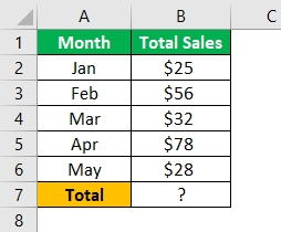
We have monthly numbers above, so to get the quick total in cell B7, press the Auto Sum shortcutThe Excel SUM Shortcut is a function that is used to add up multiple values by simultaneously pressing the “Alt” and “=” buttons in the desired cell. However, the data must be present in a continuous range for this function to function.read more key ALT + = sign.
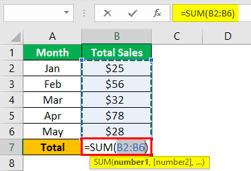
As you can see, it has inserted the SUM function in excel. Press the “Enter” key to get the result.
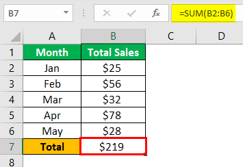
We have a quick total of the numbers above.
#2 – Data Analysis & Interpretation
The spreadsheet contains data, so telling the story behind the data is what the decision-makers need to make vital decisions in the business world. So, when the data is available with Excel, we can use MS Excel features like pivot tableA Pivot Table is an Excel tool that allows you to extract data in a preferred format (dashboard/reports) from large data sets contained within a worksheet. It can summarize, sort, group, and reorganize data, as well as execute other complex calculations on it.read more and formulas to analyze the data and interpret the numbers quickly and efficiently.
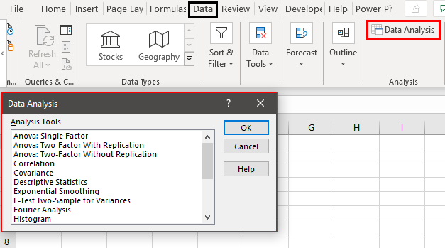
#3 – Plenty of Formulas to Work with Data
MS Excel comes with plenty of built-in functions to work with data. There are 450+ functions in excel,Excel functions help the users to save time and maintain extensive worksheets. There are 100+ excel functions categorized as financial, logical, text, date and time, Lookup & Reference, Math, Statistical and Information functions.read more, so these functions are categorized as “Financial,” “Logical,” “Text,” “Date & Time,” “Lookup & Reference,” “Math & Trig,” “Statistical,” “Engineering,” “Cube,” “Information,” and “Web.”
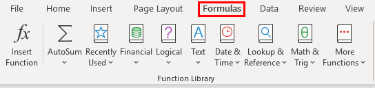
#4 – Data Organizing & Restructuring
You cannot get the data ready to use, so we can organize the data using Excel tools. We can reorganize the data according to the users’ needs.
#5 – Data Filtering
Using the option of “Filter” in Excel, we can filter the particular data from the number of rows of data. For example, we can apply a single-column filter and the filter to multiple columns to match multiple criteriaCriteria based calculations in excel are performed by logical functions. To match single criteria, we can use IF logical condition, having to perform multiple tests, we can use nested IF conditions. But for matching multiple criteria to arrive at a single result is a complex criterion-based calculation.read more to filter the data.
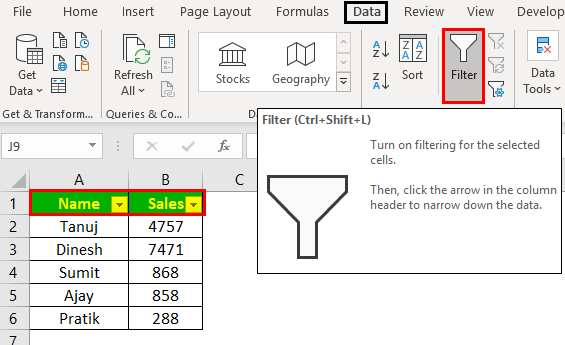
#6 – Goal Seek Analysis
When the target is set, and at a certain project stage, we may need to review that target achievement. So, using Excel, we can track all those things and identify what needs to be done in the remaining steps to achieve the desired goals.

#7 – Flexible and User-Friendly
When you compare MS Excel with other spreadsheets, you will find MS Excel as relatively friendly and flexible enough to fit the needs of the users. First, however, one needs the proper training to start things in Excel.
#8 – Online Access
Not all the time, we get the done offline, so some of the data needs to be fetched from online websites. We can import data from “MS Access File,” “Text File,” “From Web,” “From SQL Servers,” “From XML Data Import,” etc. So, getting the data to Excel is not a constraint.
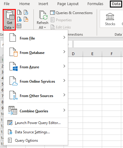
#9 – Building Dashboards
When the story behind the data is read to tell, end users may want to see those summary results in a single page view. So using MS Excel, we can build dashboards that can tell the stories in a single page view. So, not only can we build a dashboard, but it also makes the dashboard interactive.

#10 – Interactive ChartsCharts visuals are better in data depiction, but interactivity gets it better. Interactivity is when the user sees specific values in the excel chart in a more effective, efficient and crystal clear way.read more and Graphs
When the Excel formulas are applied, we can make them dynamic so that when the data range gets an addition or deletion, our formula shows the updated results instantly.
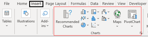
#11 – Dynamic Formulas
When the excel formulasThe term «basic excel formula» refers to the general functions used in Microsoft Excel to do simple calculations such as addition, average, and comparison. SUM, COUNT, COUNTA, COUNTBLANK, AVERAGE, MIN Excel, MAX Excel, LEN Excel, TRIM Excel, IF Excel are the top ten excel formulas and functions.read more are applied, we can make them dynamic so that when the data range gets an addition or deletion, our formula shows the updated results instantly.
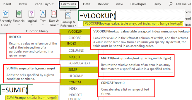
#12 – Automation Through Excel
At last, when you move to the advanced level of MS Excel, you may get bored with daily work in Excel. In that case, we can automate the reports in Excel by using the VBA codingVBA code refers to a set of instructions written by the user in the Visual Basic Applications programming language on a Visual Basic Editor (VBE) to perform a specific task.read more language.

Recommended Articles
This article is a guide to the Uses of Excel. Here, we discuss the top 12 important uses of Microsoft Excel, including getting quick totals, data analysis and interpretation, plenty of formulas to work with data, data filtering, etc., and examples and downloadable Excel templates. You may learn more about Excel from the following articles: –
- Divide Cell in Excel
- Excel Count Colored Cells
- Excel Negative Numbers
- Scroll Bars in Excel