
 This week we are celebrating Office 2010 launch at chandoo.org
Office 2010 [download beta version | purchase], the latest and greatest version of Microsoft Office Productivity applications is going to be available worldwide in the next few weeks. I have been using Office 2010 beta since November last year and recently upgraded my installation to the RTM version (Ready to Manufacture, a version that is final and used for burning CDs that MS sells).
I was pleasantly surprised when I ran Microsoft Excel 2010 for first time. It felt smooth, fast, responsive and looked great on my comp.
This week, we are going to celebrate launch of Office 2010 by learning,
- What is new in Excel 2010
- Introduction to Excel 2010 Spark-lines
- New Conditional Formatting Features in Excel 2010
- Making your own ribbon in Excel 2010
- Using the Backstage View in Excel 2010
Leave a comment to win a copy of Office 2007 – Home & Student Edition
(with free upgrade to Office 2010 in June)
What is new in Excel 2010?
There are a ton of new and cool features in Excel 2010. My favorite new features are,
Sparklines
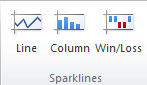
These are small charts that can be shown inside a cell and are linked to data in other cells.You can insert a line chart, win-loss chart or column chart type of spark line in excel 2010. They add rich information analysis capability to mundane tables or dashboards. We learn more about using them in tomorrows article.
[meanwhile: Learn how you can make sparklines in earlier versions of Excel]
Slicers

Slicers are like visual filters. They are an easy way to slice and dice a pivot table (what is a pivot table – tutorial). A sample slicer at work is shown above.
Improved Tables & Filters

When working with tables in Excel 2010, you can see the table filtering & sorting options even when you scroll down (the column headings – A,B,C… change to table headings)
[Related: Introduction to Excel Tables]
Also, in Excel 2010, data filters have a nifty search option to quickly search and filter values you want. (I still prefer the excel 2003 style one click filtering).
New Screenshot Feature:

Now, using Excel (or any other Office 2010 app) you can grab a screenshot of any open window. This could be very useful for those of us in teaching industry as you can quickly embed screenshots in to your teaching material (like slides or documents).
Paste Previews:

There are a ton of cool paste features buried in the Paste Special Options in earlier versions of Excel. MS has bought all these to fore-front with Paste Previews feature in Office 2010.
Improved Conditional Formatting:

Excel 2010 added a lot of simple but effect improvements to conditional formatting. One of my favorites is the ability to have solid fill in a cell based on the value in it. This provides an easy way to create in-cell bar charts.
Customize Pivot Tables Quickly

Now you can easily change pivot table summary type and calculation types from Pivot Table “Options” ribbon in a click (learn how to do this in Excel 2007 and earlier).
Also you can do what-if analysis on Pivots (I am yet to try this feature).
Customize Add-ins from Developer Ribbon

In Excel 2007, if you want to customize or add a new add-in, you have to circumnavigate cape of good hope. But Excel 2010 makes it a pleasant experience again. There are two buttons, right on developer ribbon tab using which you can quickly add, change any add-ins.
(also, it seems like developer ribbon is turned on by default, which is pretty cool.)
Customize Ribbons and Define your own Ribbons

One the most beautiful and powerful features about Office products is that you can customize them as you want. You could easily add menus, change labels, and define toolbars the way you like to work. It made us feel a little powerful and awesome. Then, for some reason, MS removed most of these customizations in Office 2007 leaving us frustrated and powerless. Thankfully, they restored some of that in Office 2010. In this version of office, you can easily add new ribbons or customize existing ribbons (by adding new groups of tools).
One File Menu to Rule them all
One of the biggest WTFs in Excel 2007 is Office Button. It wasn’t immediately clear for most of us, how we should save or work with existing files as everything was hidden behind the office button. Office 2010 rectified that problem beautifully by restoring “File” menu. But the engineers at MS didn’t stop there. They also added a host of other powerful features to the file menu and branded it as “backstage view”. Kudos! [Learn more about File Menu and Backstage view on this Friday]
Many more new features:
Not just these, there are many more subtle UI enhancements, features and improvements in Excel 2010 (and all other Office products). For eg. macro recorder now works with charts too, you can double click on chart elements to format them, you can collapse ribbon with a click, there is a new UI for solver, lots of statistical formulas have improved accuracy, there is exciting PowerPivot Add-in (my review of powerpivot) to let you do poweful BI and Analysis work right from Excel and many more. [read about all changes in Excel 2010 at TechNet]
You could win a Copy of Office 2010 – Home & Student Edition
Through out this week, I will be posting about Excel 2010’s new features and how you can use them to be even more awesome. I have 2 3 free licenses of Office 2007 Home & Student Edition (free upgrade to Office 2010) to giveaway.To qualify, all you need to do is drop a comment on any of the 5 posts this week.
The contest is sponsored by Microsoft and winners will be chosen randomly.
Addendum: I got 3 licenses to giveaway. 2 of them for Indians and one for a lucky international reader.
So, what are you waiting for? Go ahead and tell me what your favorite feature in Excel 2010? Leave a comment to win an Office license.
Things to do:
Share this tip with your colleagues

Get FREE Excel + Power BI Tips
Simple, fun and useful emails, once per week.
Learn & be awesome.
-
101 Comments -
Ask a question or say something… -
Tagged under
Excel 2010, excel tables, john walkenbach, Learn Excel, Microsoft Excel Conditional Formatting, Office 2010, pivot tables, powerpivot, reviews, ribbon, slicers, solver
-
Category:
Featured, Learn Excel

Welcome to Chandoo.org
Thank you so much for visiting. My aim is to make you awesome in Excel & Power BI. I do this by sharing videos, tips, examples and downloads on this website. There are more than 1,000 pages with all things Excel, Power BI, Dashboards & VBA here. Go ahead and spend few minutes to be AWESOME.
Read my story • FREE Excel tips book


Excel School made me great at work.
5/5

From simple to complex, there is a formula for every occasion. Check out the list now.

Calendars, invoices, trackers and much more. All free, fun and fantastic.

Power Query, Data model, DAX, Filters, Slicers, Conditional formats and beautiful charts. It’s all here.

Still on fence about Power BI? In this getting started guide, learn what is Power BI, how to get it and how to create your first report from scratch.
Related Tips
101 Responses to “What is new in Microsoft Excel 2010? [Office 2010 Week]”
-
Hi,
For me, the best new feature has got to be sparklines. I love the idea of putting a bar graph into a cell using =rept, and now with sparklines, this idea can be expanded upon and greatly imroved. Roll on for the June launch!
Phil
-
When I see those Excel 2010 features I can only imagine it is so close to being perfect calc sheet… Creating my own tab is the only feature I was missing in almost perfect 2007, and now we have it. And those gadgets like sparklines or slicers only make this Excel better.
-
 Subhash says:
 Hi Chandoo,
Can you also include the online collaboration aspects of Excel 2010 in your preview?Regards,
Subhash -
Rakesh says:
Hi,
I think Sparklines are the best feature that has been added to Excel 2010.Thanks!
-
Saurabh says:
Purna,
To me the best feature is definitely the screen shot. You say it is good for people in teaching industry and I feel it is equally useful in IT industry where again you have to educate your customer. -
Kenjin says:
Hi Chandoo,
I’ve discovered your blog recently when I start to be interested in data visualization and dashboard design (I’m a young graduate). I’ve learnt a lot about Excel thanks to you.
All these new features are interesting, the less being the screenshot maybe. I am especially interested in paste previews, customization of pivot tables and improved conditional formatting. The intentions behind sparklines are good, but the features seem poor compared to VBA programs.
What is interesting for data analysis, I think, is Power Pivot. It makes exploratory analysis much more easier, especially with the integration of data from different sources. For sure it won’t be as good as Tableau Software, but for business people who already have a fair knowledge of Excel, they don’t have much to learn.
Regards!
-
Victor says:
Thanks for the always useful post Chandoo!
I hope I win -
Martin says:
Thanks to additional features, MS Office will still remains the king of office software suites!
-
Squiggler says:
Without doubt the biggest aid to my productivity is being able to create my own tabs! While many of us use a subset of each tab on a regular basis, its sometimes infuriating to have to switch several times to find each feature, now I just create a tab with the Items I use the most and cut down on the time! The other nice Item is the availability of Paste Special options from the right click menu, so now I can preview the options by hovering before I paste and Undo as I have countless times!
-
Raj says:
Looks like Excel 2010 is good for basic users also. Hope it will help me to build some good dashboard. However, how is its reliability compared to a standard statistical package?
-
Pedro Roenick says:
Nice quick review.
Greetings from Brazil. -
Nisar says:
The favourite features in Excel 2010 is as follows
1) there are serveral new smart art designs
2) the Slicer is indeed cool
3) The customization of ribbon -
Reyov says:
Hi Chandoo,
Without a doubt, I think the best new feature will be the sparklines. It’s going to make my life easier doing some dashboards.
Thanks! -
I like the (re-)introduction of Customising and Defining your own Ribbons, and the File menu returning is also great.
Love the blog, Chandoo, Keep it up, or as we say in Ireland, «Bail o Dhia ar an obair» (directly translates to: «May God bless the work»), A general greeting given when you see someone working hard at something, to praise him and his efforts.
-
dan l says:
Chandoo:
I’m curious. How does the built in sparklines feature compare to SFE? I expect that it will be less robust but far easier to email out to folks. Why I just had a «forgot to deactive the formulas» incident today.
A little embarrassing.
-
Dan, look at the link in my comment a few posts up
-
Tom says:
Chandoo,
You’re getting me excited for 2010. I don’t know when I’ll get a copy at work because I have a relatively new computer and it came with 2007 installed. I can’t seem them paying for the upgrade just yet (which is why I’d love to win a copy) 🙂 I really like the idea of the customized ribbons the most, and I also really like the paste preview.
One problem that I have, in using the latest version of Excel, is the distribution of my work to folks with older versions. Hopefully, it won’t be long before the majority of our staff have at least 2007.
Thanks for all you do!
Tom (U.S.A.)
-
Steve says:
Bring on the sparklines!
-
Michael says:
My favorite is Slicers followed by Sparklines.
-
Lisa says:
I love the data bars in conditional formatting and the slicers.
-
Robert K says:
While PowerPivot & Slicers enhance analysis capabilities, and Sparklines are great (even though I learned in-cell charting from you on CHANDOO.ORG), the most useful thing for me has to be the new % of Parent… options in PivotTable summaries. Previously, there was not a simple way to present these calculations without significantly altering the layout of my PivotTables.
I’ve been a reader since Jan 2009…thanks for the nice Excel 2010 preview and all the great info!
-
Karen says:
If I am lucky enough to win a copy of 2010, I will be happy to post about my favorite features. 🙂
-
CMT says:
Glad to see ribbon customization beyond just the QAT. Now we won’t be so hamstrung by Excel engineers’ vision of which buttons we’ll want when, and can possibly go back to being productive.
-
Geoff says:
It’s sad, but Paste Special is by far the most commonly used attribute on Excel for me. Allowing a preview will be exactly what I need. Also sad is that we have just upgraded to 2007 and I on that schedule, we should be on 2010 by 2013 🙂
-
jeff weir says:
I’m going to double my chances of winning.
-
jeff weir says:
There, just doubled my chances of winning
-
Ivan says:
It looks like Excel 2010 is making great leaps forward. Too bad we are just getting around to testing Excel 2007 at work.
-
chrisham says:
The PowerPivot add-in and the Sparklines ought to be by far the best features in Excel 2010.
-
jeff weir says:
Ivan…you don’t test Excel 2007. Rather, Excel 2007 tests you.
-
Oscar Noriega says:
Hello,
The restoration of the «File» menu is nice feature and the Sparkline feature is a nice addtion also.
Thanks
-
I definitely agree with the other folks here. Sparklines are definitely a great new feature in Excel 2010. They will add a powerful visual element for Excel dashboards that is not present even in many of the more powerful Web-based business intelligence tools. They will give us the ability to see a lot of information (for example, subtle trends and patterns in the data) that was previously too hard to build by hand.
-
laguerriere says:
Hi Chandoo,
well, I’m rather a «silent» fan of your page, but this time I need to say: awesome post!!! Now there is again a thing I ‘ll dream of to have!! Although I was kind of sceptic about Office 2007, i am now used to it and sometimes it helped me much more than excel 2003. By the way, do you know any good blog for Powerpoint 2007 Tips? It’s so annoying that some features disappeared , it was much easier to double-click on an object.
Thank you so much!
All the best to you and your family,
La Guerrière -
Jay Venator says:
Best new feature: All! in 2007 version I was missing every feature you covered. I need to upgrade, lets see if I win first.
-
I’ve been using the 2010 beta for several months. I’m having trouble understanding how slicers are any different than simply selecting the checkboxes in each pivot table’s field — don’t they both get you to the same place? Is there some value to slicers that I am missing?
-
jay says:
Favorite feature is Sparklines. It helps me to analyse data faster and better. It also provides me a quick view of information without resorting to opening another chart on top of the sheet.
Thanks pls count me in the draw. -
Patrick says:
The new PivotTable features are much-needed. I was using PivotTables today and could have really used that feature.
-
Rob says:
There seems to be a general reluctance for people to upgrade to 2007/10 because of the ribbon. Where I work, the IT department doesn’t like to install it because users complain. Once I’d tried it and re-learned a few things, I prefered it. Hopefully these new features will win over even more converts.
Rob -
Mark S says:
Great tips Chandoo! I am going to download the Beta on my home system to start to understand the product. I like what you have described so far. It kinda makes you think if your upgrading to bypass 2007 and go straight to the top product.
Thanks for you timely updates.
Mark S.
-
Mark S says:
Great article on 2010! going to download the beta and get into it.
Thanks for the timely update.
Mark S.
-
Frederick says:
My favourite new feature should be slicers. We must remember that the best Excel output is for people who don’t know know Excel to be able to look at what it is and have it explain something.
This feature will help alot in data visualisation.
-
dan l says:
Jesus Alex. I’m an idiot. I didn’t even notice your comment with the linky until you posted it now. Thank you for the detailed commentary.
It looks like SFE is still the way to go for a ‘hard’ project. The day to day stuff can be done in excel 2010.
-
Roji says:
My current work deals with a lot of data and it’s analysis. I use VBA and charts/graphs on a regular basis. To me, the Sparklines, Slicers, improved Filters, improved Conditional Formatting & Pivots functionality is a very welcome move.
What I would like to see in Excel is the fuel-gauge/speedometer type of charts. I wonder why Microsoft hasn’t considered providing this as an option yet. I have seen the various hacks as to how this can be achieved, but it would have been a lot better if it was provided as a built-in option. -
Marrosi says:
The customisation of the ribbon makes life much easier (….makes Excel-life muche more Excellent …) and certainly improves productivity.
-
joe says:
i like spark line in ofice 2010
-
Cyril Z. says:
Hello Chandoo,
As usual your article is very insteresting and detailed.
I’m very found of the following 3 points :
— Customisation of the ribbon : I’ve struggled in XL2007 to understand why I eventually lose the ribbon when saving… HOpe this will ease my life (what? too much expectations ? 🙂
— File Menu reappears ! Was really not found of the button instead
— Table headers in columns, but I wonder how this will work with multiples tables… :-/Have fun in your new carrier 🙂
Cyril
-
Abdul Kader says:
Hi Chandoo,
I was transfering from my house from East Jerusalem to Ramallah,Palestine for the last week and the internet was disconnected, you are the first that I am in contact after resuming internet.As usual you are superior from all aspects simple English, good presentation, in my opinion they have done a lot of improvements don’t forget the new functions SUMIFS …ETC
-
Scaffdog845 says:
Hi Chandoo,
Many of the users I help to support are afraid that our company is going to want to change to 2010. They had a heck of a time and still struggle with the changes from 2003-2007. Personally I think 2010 will simplify some of the off the wall things i was working to get 2003+2007 to do.
Keep the posts coming.
-
A lot of old proficient users didn’t move to 2007 because of the inability to customize the toolbars (now Ribbons).
As Chandoo says above, you can customize the Ribbon. You can create your own tabs or groups inside those tabs.
So for those old-menu-fans, the menu is definitely gone, the floating toolbars are gone too. Now the customization is back (Microsoft listens users).
The Ribbon remains.
I am sure reticent people (those who says: my time is too valuable to spend multiple-clicking when one click used to do, I want to replace the new Ribbon with the Classic menu interface) will move to 2010 once they confirm the program brings this so-expected capability.
-
GCD says:
Sparklines, definitely. Gonna be a giant pain waiting for the world to catch up with the new formats, though.
-
Amit Arora says:
For me all the new data analysis and data visualization tools do a world of good. Sparklines and slicers would stop us from looking out for some free add-on to do that work.
-
Macao says:
Hi, I think that the sparkline feature is the best new thing in Excel 2010.
-
Alexandre says:
Hey,
Great information!!. Would love to win this to use here in Brazil.
Let’s wait and see.
-
Abhishek Jain says:
the option i liked the most is quick customization of Pivot Tables….would help in reducing a lot of time wastage in data analysis for me…m excited to try out MS office 2010 now!!
-
Savannah says:
Chandoo, your website is marvelous and your tool-set has truly made me an Excel rockstar in my office so many, many thanks.
I’ve been so fortunate to be working with an MS representative this week testing XL2010 and have already informed my boss that I will be a very crabby camper if we do not purchase and implement.
Thanks again!
-
Great and very interesting resume about what’s coming for us!
Best Regards -
Savannah says:
Hi Chandoo, love the site — I get teased for all the great things I say about you but I don’t care. You are a hero!
Also looking and evaluating XL2010 for company purchase — digging so many aspects.
Thanks so much
-
Steve says:
I didn’t realize the amount of new tweaks in 2010. Very nice. Fun to play with Sparklines in particular. The screen cap tool is quite useful, too.
-
Gaurav says:
I love how in Excel 2010 they have replaced the old conditional sum wizard with the function wizard that includes SUMIF and SUMIFS functions.
-
Sam says:
You must be kidding. I am now unable to construct what I used to do and I work professionally with Excel since 1988.
-
Hui says:
@Sam
Can you post an example of something that you can’t do now ?
-
-
-
The top two features for me are:
1. Sparklines
2. Gradient Fill in Conditional formatting.When combined with Slicers, they can prove to be a formidable tool for dashboards and such.
-
Hi will love to have free copy of MS Office 2010 in order to move faster with your posts……thanks
-
mark says:
This is my registration for your giveaway.
-
There is always room for improvement. As usual I was expecting new features. Slicers and custom user ribbons will help me a lot. Great work Microsoft excel team!
-
Steve Berlin says:
I like the slicers and the sparklines. I have the sparkline addon already but it will be nice so others will be able to use my worksheets if they have office 2010
-
Karthik G says:
Chandoo, I liked the powerpivot add in that goes with 2010, its just great.
-
Vinu says:
I like
customizing toolbar
and Conditional formatting features in 2010 version.
Waiting to get hang on Excel 2010!! -
nitesh says:
sparklines and conditional formatting features are the best ones
i never tried this sparklines feature in the beta version of 2010
gr8 post -
Mark in Canada says:
I downloaded the Office 2010 Beta trial last year when you first mentioned it and have been surprised at how much Microsoft has optimized the applications — the user interface design is very well done and the responsiveness is snappy. I am glad to say that I haven’t had any of the crashes in Excel 2010 🙂 that I have had with PowerPoint 2010… 🙁
And I am (finally) starting to get used to the ribbon… some things still take more clicks, which is disappointing.
Here’s hoping that I’m the international winner of the Office 2010 license. 🙂
-
Miguel C says:
I like sparklines! I’m still on Office 2003. Please pick me to win Office 2010!
-
Abhishek says:
Good new features and apparently the best part is they (Microsoft guys) are reading the mindset of the Excel users very quickly by providing such niche features in every release to reduce the burden of coding and applying complex logic.
I’m not using Office 2010 but I wish sometime in future when it will be implemented by my company, I’ll be able to enjoy all such great features.
Thanks for this post it’s really nice to read about all such cool features.
-
Dear Chandoo,
I have downloaded office 2010 and felt it was smooth and good.
Spark lines ands Pivots and good graphing tools (even in 2007) are definite value additions.
I am yet to try slicers.
Thanks for the post.I will try all the new features.
Regards
Mahesh -
John Pomfret says:
Hi Chandoo,
It’s difficult to pick a favourite but the conditional formatting is certainly up there in the list.
I recently resigned from my job as an excel developer after 9 1/2 years at the company.
The plan was to take some time out and sort out my priorities.
May 31st was my final day of employment (a Bank holiday here in the UK). At 2pm on June 2nd I got a phone call asking if I wanted to do some work for them as tehy were unhappy with the contractor. I did go for a meeting and am waiting to hear. I think I deserve the prize for being a masochist!
John -
Oliver Montero says:
The favorite features in Excel 2010:
1) The Slicer is indeed cool
2) The customization of ribbon (At last MS)
3) PowerpivotFor me Excel 2010 is to Excel 2007 what Windows 7 was to Windows Vista. What it should have been for the first time.
-
Santosh Maturi says:
how to lock the image in excel sheet one cell
Regards
Santosh Maturi -
[…] Tom (this Tom) […]
-
Jeff says:
If I upgrade from Excel 2007 to 2010 will I lose my macros?
Thanks.
-
Geeky Mummy says:
Sparklines — a tool given to us to wipe out the all too common glazed over eyeball syndrome — often contracted when looking at tables upon tables of data.
-
Chris says:
Chandoo,
Fantastic site your sharing of knowledge is great. Still stuck using 2003… salivating again at the thought of taking an even larger leap when my company does choose to upgrade. I just hope they finally take the leap!!
Cheers,
Chris -
Hui… says:
@Jeff, No
As an asisde, the macro facilities in 2010 are much better than in 2007. -
Tommi says:
I am also waiting for the 2010 version release. Hope it will be also available via MSDN AA.
Btw, Chandoo, great blog 🙂 -
Lynn says:
I have upgraded to Excel 2010 due to PowerPivot, Slicer, and Sparklines. I am the only one to have this version at work!
-
Subie says:
Can we finally put Office 2007 behind us???
-
Abe Asanji says:
Hi Chandoo,
I had not yet installed Office 2010 Beta. Is it still possible for me to downgrade it back to Office 2007 if Office 2010 expires?
-
@Abe.. As I mentioned about, do not upgrade your office 2007 to 2010. Instead, choose the option (install only) that will keep both versions working. This way, when beta expires you can uninstall 2010 and nothing breaks.
-
-
Akash says:
Chandoo, I have 2003, 2007 and 2010 Beta installed and working fine on the same machine. Would MS be upgrading the Beta to RTM version on its own?
-
@Akash… No, the beta will just expire at oct 2010 unless you manually upgrade to full version of Office 2010. It is available for purchase now.
-
-
Kalee says:
I just recently purchased Microsoft Home and Student 2010. I am having a horrible time with Excel. I can’t seem to make more than a few data entries into cells without Excel freezing up and crashing. I’ve never seen Excel behave so erratic before. Any suggestions?? Thanks!
-
Akash says:
Chandoo, Who are 3 lucky ones to win the licences of office 2010? They must be congratulated on this forum.
-
Hello Chandoo,
Nice article on the new features… -
Robapottamus says:
Gidday Chandoo
cheers for the write up. lookin forward to 2010, especially the sparklers and slicers. These will be some nifty additions to my reports — maybe enough to impress the boss for a payrise???
-
Harshad says:
My Tab…awesome feature in Excel 2010….Customization at its best…
Previous version lacked that feature…for Data analysis people this will be most useful feature…
Nice Job Chandoo… I am you fan dude…. -
jayank2000 says:
MS Office 2010 is a great upgrade from Office 2007. I personally still have Office 2003. Cannot wait to grab a copy of Office 2010.
-
renaud says:
Hi
Have you had the chance to try out the what if analysis on pivot feature?
Thanks
Renaud
-
wow, still use microsoft office 2007 in my home. but after seeing this description, i should put my 2007 to 2010..hihi
-
Sarah Black says:
Hi! I am a college student, and one of my classes is a computer app class. I have office 2007, but my instructor uses 2010 for her teachings. I am not very familiar with excel, but I do have some assignments coming up using excel. I suppose it is going to be a little more difficult for me to get the hang of it if she is teaching us from office 2010 and I have 2007. I am sure I will survice long enough till I can upgrade to office 2010. However, I am liking what I am seeing in the office 2010.
-
april says:
what are the 25 functions of excel
-
ButchPrice says:
One word. Slicers. They are awesome. Simple and clean when the correct slicer is used. I am learning volumes with the courses, and found myself being referred to in an important meeting as the «Spreadsheet Master» by a colleague. Nice.
Thank you for all your efforts.
Do you provide a course or study plan dealing with workbooks interacting with other workbooks? I have many workbooks created from a common template that I would like to search for and display, based on key common cells, and extract the 1st sheet of each to compile into one large file of sheets.
Leave a Reply
Содержание
- Microsoft Excel 2010 (краткий обзор)
- Лента
- Открытие книги Excel 2010 в более ранних версиях Excel
- Восстановление предыдущих версий документов
- Быстрое сравнение списков данных
- Улучшенное условное форматирование
- Правила Условного форматирования и Проверки данных
- Улучшенная надстройка «Поиск решения»
- Новый фильтр поиска
- Фильтрация и сортировка независимо от расположения
- Ввод математических формул
- Скачать Microsoft Excel 2010 бесплатно
- Microsoft Excel 2010 на компьютер
- Excel 2010 —
- Getting Started with Excel
- Excel 2010: Getting Started with Excel
- Lesson 1: Getting Started with Excel
- Introduction
- Getting to know Excel 2010
- The Excel interface
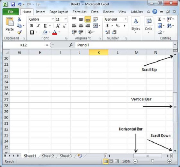
- Name Box
- Quick Access Toolbar
- Zoom Control
- Page View
- Horizontal Scroll Bar
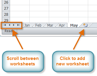
- Worksheets
- Formula Bar
- Column
- Ribbon
- Working with your Excel environment
- The Ribbon
- To customize the Ribbon:
- To minimize and maximize the Ribbon:
- The Quick Access toolbar
- To add commands to the Quick Access toolbar:
- Backstage view
- To get to Backstage view:
- Options
- Save & Send
- Save, Save As, Open, and Close
- Recent
- Creating and opening workbooks
- To create a new blank workbook:
- To open an existing workbook:
- Compatibility mode
- To convert a workbook:
Microsoft Excel 2010 (краткий обзор)
history 25 октября 2014 г.
Статья посвящается тем пользователям, которые продолжают работать в версии MS EXCEL 2007, но уже подумывают о переходе на новую версию.
Отличия MS EXCEL 2010 от версии 2007 года не столь радикальные по сравнению с отличиями MS EXCEL 2007 от MS EXCEL 2003 (см. статью Microsoft Excel 2007 (основные отличия от EXCEL 2003) , но все же различия существенные — рассмотрим основные из них.
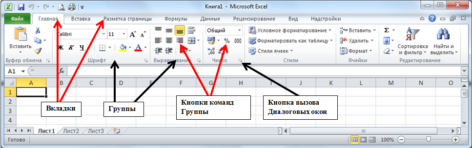
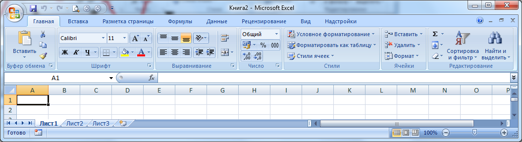
Лента
Лента — пользовательский интерфейс, пришедший на смену панелям инструментов еще в версии MS EXCEL 2007 . Лента представляет собой широкую полосу в верхней части окна EXCEL, на которой размещаются основные наборы команд, сгруппированные отдельных вкладках.
Лента в EXCEL2010
Лента в EXCEL2007
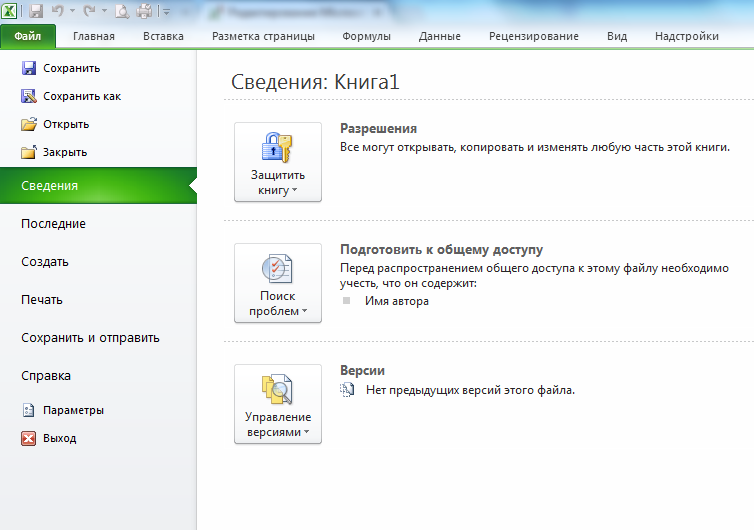
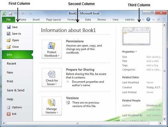
Сравним ленту в EXCEL2010 и в EXCEL2007. Основным отличием является то, что Вкладка Файл (File), пришедшая на смену кнопки Office (в EXCEL 2007), открывает так называемое представление Microsoft Office Backstage, которое содержит команды:
- для работы с файлами (Сохранить, Открыть, Закрыть, Последние, Создать);
- для работы с текущим документом (Сведения, Печать, Сохранить и отправить);
- для настройки Excel (Справка, Параметры).
В приложении Excel 2007 можно было настроить панель быстрого доступа, однако не было возможности создавать собственные вкладки и группы на ленте. В Excel 2010 можно создавать настраиваемые вкладки и группы, а также переименовывать и переупорядочивать встроенные (подробнее здесь ]]> http://office.microsoft.com/ru-ru/excel-help/HA010355697.aspx?CTT=5&orig. ]]> ).
Открытие книги Excel 2010 в более ранних версиях Excel
Чтобы обеспечить возможность работы над документом MS EXCEL2010 в более ранних версиях Microsoft Excel, можно воспользоваться одним из двух способов:
- Книгу, созданную в MS Excel 2010, следует сохранить в формате, полностью совместимом с Excel 97-2003 (xls). Она, естественно, откроется в более ранних версиях EXCEL. Конечно, для пересохранения файла понадобится версия MS EXCEL 2010. Этот подход можно использовать, если, например, на работе имеется EXCEL 2010, а дома — более ранняя версия.
- Загрузить Пакет обеспечения совместимости форматов файлов Microsoft Office 2010 для программ Office Word, Excel и PowerPoint . Он позволяет открывать, редактировать и сохранять книги Excel 2010 в предыдущих версиях Microsoft Excel без необходимости сохранять их в формате предыдущей версии или обновлять версию Microsoft Excel до Excel 2010.
Совет : Пакет обеспечения совместимости можно скачать на сайте Microsoft ( ]]> http://www.microsoft.com/ru-ru/download/confirmation.aspx?id=3 ]]> ) или набрать в Google запрос Пакет обеспечения совместимости форматов файлов Microsoft Office 2010 для программ Office Word, Excel и PowerPoint .
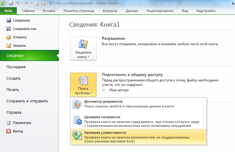
Естественно, в файле созданном в MS EXCEL 2010 могут содержаться элементы, у которых нет аналогов в более ранних версиях. Для того чтобы убедиться в том, что книга Excel 2010 не содержит несовместимых элементов, способных вызвать значительную потерю функциональности или незначительную потерю точности при открытии в предыдущих версиях Excel, можно запустить средство проверки совместимости. Во вкладке Файл выберите команду Сведения и затем нажмите кнопку Поиск проблем . В меню кнопки выберите команду Проверка совместимости .
Восстановление предыдущих версий документов
В EXCEL 2010 теперь можно восстановить версии файлов, закрытые без сохранения изменений. Это помогает в ситуациях, когда пользователь забыл сохранить файл вручную, случайно были сохранены ненужные изменения или просто возникла необходимость вернуться к одной из предыдущих версий книги. ]]> Ознакомьтесь с дополнительными сведениями о восстановлении файлов ]]> .
Быстрое сравнение списков данных
В приложении Excel 2010 новые компоненты (такие как спарклайны и срезы), улучшения сводных таблиц и других существующих функций помогают выявлять закономерности и тренды в данных.
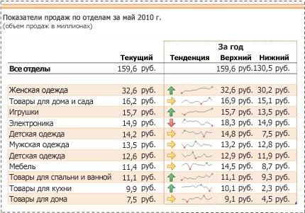
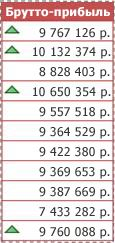
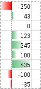
Спарклайны — маленькие диаграммы, помещающиеся в одну ячейку, — позволяют визуально отображать тренды непосредственно рядом с данными. Поскольку спарклайны показывают тренды на ограниченном пространстве, с их помощью удобно создавать панели мониторинга и другие аналогичные компоненты, демонстрирующие текущее состояние дел в понятном и наглядном виде. На рисунке ниже показаны спарклайны в столбце «Тренд», позволяющие моментально оценить деятельность каждого из отделов.
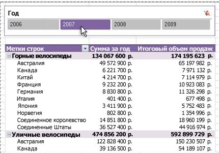
Срезы — это визуальные элементы управления, которые позволяют быстро и интуитивно фильтровать данные в сводных таблицах в интерактивном режиме. Вставив срез, можно с помощью кнопок быстро выделить и отфильтровать данные, представив их в нужном виде. Кроме того, если к данным сводной таблицы применено более одного фильтра, больше не нужно открывать список, чтобы выяснить, что это за фильтры: они отображаются непосредственно на срезе. Срезы можно форматировать в соответствии с форматом книги и повторно использовать их в других сводных таблицах, сводных диаграммах и функциях куба.
Улучшенное условное форматирование
С помощью условного форматирования можно легко выделять необходимые ячейки или диапазоны, подчеркивать необычные значения и визуализировать данные с помощью гистограмм, цветовых шкал и наборов значков. Впервые появившиеся в Office Excel 2007 наборы значков позволяют помечать различные категории данных в зависимости от заданного порогового значения. Например, можно обозначить зеленой стрелкой вверх большие значения, желтой горизонтальной стрелкой — средние, а красной стрелкой вниз — малые. В приложении Excel 2010 доступны дополнительные наборы значков, включая треугольники, звездочки и рамки. Кроме того, можно смешивать и сопоставлять значки из разных наборов и легко скрывать их из вида — например, отображать значки только для показателей высокой прибыли и не показывать их для средних и низких значений.
В приложении Excel 2010 доступны новые параметры форматирования гистограмм. Теперь можно применять сплошную заливку и границы, а также задавать направление столбцов «справа налево» вместо «слева направо». Кроме того, столбцы для отрицательных значений теперь отображаются с противоположной стороны от оси относительно положительных.
Правила Условного форматирования и Проверки данных
Задавая критерии для условного форматирования и правил проверки данных , теперь можно ссылаться на значения на других листах книги.
Улучшенная надстройка «Поиск решения»
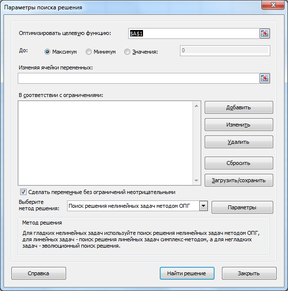
В состав приложения Excel 2010 входит новая версия надстройки «Поиск решения», позволяющая выполнять анализ «что если» и находить оптимальные решения. Последняя версия этой надстройки обладает улучшенным пользовательским интерфейсом Evolutionary Solver, основанным на алгоритмах генетического анализа, для работы с моделями, в которых используются любые функции Excel. В ней предусмотрены новые глобальные параметры оптимизации, улучшенные методы линейного программирования и нелинейной оптимизации, а также новые отчеты о линейности и допустимости.
Новый фильтр поиска
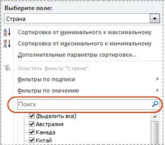
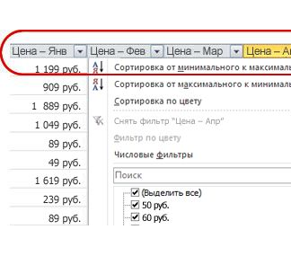
При фильтрации данных в таблицах Excel, сводных таблицах и сводных диаграммах доступно новое поле поиска, позволяющее находить нужные данные в больших списках. Например, чтобы найти определенный товар в каталоге, содержащем более 100 000 позиций, просто начните вводить искомое наименование — и подходящие элементы сразу же появятся в списке.
Фильтрация и сортировка независимо от расположения
При прокручивании длинной таблицы Excel ее заголовки заменяют собой обычные заголовки листа, находящиеся над столбцами (только для таблиц в формате Excel2007 ). Кнопки автофильтра теперь остаются видимыми вместе с заголовками таблицы в ее столбцах, что позволяет быстро сортировать и фильтровать данные, не прокручивая таблицу для отображения ее верхней части.
Ввод математических формул
В Excel 2010 с помощью новых инструментов редактирования уравнений можно вставлять на листы распространенные математические уравнения или создавать свои собственные, используя библиотеку математических символов. Новые уравнения можно также вставлять в текстовые поля и другие фигуры (не в ячейки). Чтобы вставить уравнение, на вкладке Вставка в группе Символы щелкните стрелку рядом с кнопкой Формула .
Источник
Скачать Microsoft Excel 2010 бесплатно
Категория:
 |
Офисный пакет |
| Windows XP, 7, 8, 10 | |
| 32 bit, 64 bit, x32, x64 | |
| Компьютер | |
| На Русском | |
| Бесплатно | |
| Microsoft |
Поддерживаемые ОС:Разрядность:Для устройств:Язык интерфейса:Версия:Разработчик:
Microsoft Excel 2010, это обновленное издание программы из офиса, для создания и редактирования электронных таблиц. С помощью табличного редактора, пользователь будет фиксировать информацию и вычислять сложные примеры, не выходя из программы, и не напрягая мышление.
Microsoft Excel 2010 на компьютер
Программа Эксель наглядно представит большие объемы информации в понятной таблице и поможет сделать анализ или расчет. Получите четкое представление об информации: упорядочивайте, визуализируйте и извлекайте нужную информацию еще проще, благодаря полезным инструментам и командам. Сотрудничайте с легкостью, облачное хранилище OneDrive объемом 1 ТБ позволит выполнять резервное копирование, совместное использование и совместное редактирование книг с сенсорных устройств.
Используйте Excel на ходу, просматривайте и редактируйте файлы на работе, дома или в другом месте с помощью мобильных приложений для iOS, Android и Windows. Цените и экономьте время, поскольку Microsoft Excel изучает шаблоны пользователя и систематизирует информацию. С легкостью создавайте новые таблицы или начните с шаблонов. Используйте современные формулы для выполнения расчетов. Представляйте информацию в привлекательном виде с помощью новых диаграмм и графиков. Используйте таблицы и форматирование, чтобы лучше понимать написанное. Делитесь созданной книгой и работайте вместе быстрее над последним выпуском в режиме прямой трансляции времени. Работайте с файлом Excel на мобильном устройстве или компьютере.
Источник
Excel 2010 —
Getting Started with Excel


Excel 2010: Getting Started with Excel
Lesson 1: Getting Started with Excel
Introduction
Excel is a spreadsheet program that allows you to store, organize, and analyze information. In this lesson, you will learn your way around the Excel 2010 environment, including the new Backstage view, which replaces the Microsoft Office button menu from Excel 2007.
We will show you how to use and modify the Ribbon and the Quick Access toolbar, as well as how to create new workbooks and open existing ones. After this lesson, you will be ready to get started on your first workbook.
Getting to know Excel 2010
The Excel 2010 interface is similar to Excel 2007. There have been some changes we’ll review later in this lesson, but if you’re new to Excel first take some time to learn how to navigate an Excel workbook.
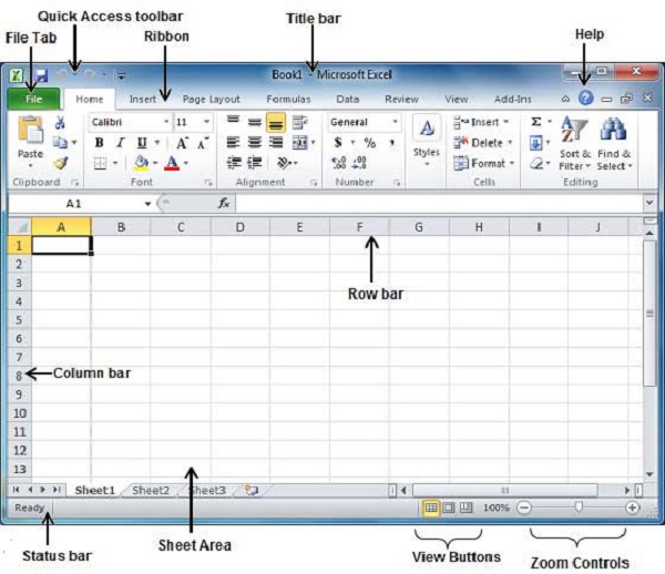
The Excel interface
Click the buttons in the interactive below for an overview of how to navigate an Excel workbook.
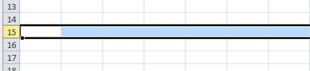
A row is a group of cells that runs from the left of the page to the right. In Excel, rows are identified by numbers. Row 15 is selected here.
Name Box
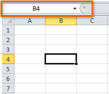
The name box tells you the location or the name of a selected cell. In the image below, cell B4 is in the name box. Note how cell B4 is where column B and row 4 intersect.
Quick Access Toolbar
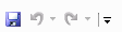
The Quick Access toolbar lets you access common commands no matter which tab you are on. By default, it shows the Save, Undo, and Repeat commands. You can add other commands to make it more convenient for you.
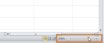
Zoom Control
Click and drag the slider to use the zoom control. The number to the left of the slider bar reflects the zoom percentage.
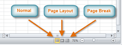
Page View
There are three ways to view a spreadsheet. Click a page view button to select it.
• Normal view is selected by default and shows you an unlimited number of cells and columns. It is highlighted in this image.
• Page Layout view divides your spreadsheet into pages.
• Page Break view lets you see an overview of your spreadsheet, which is helpful when you’re adding page breaks.
Horizontal Scroll Bar
You may have more data than you can see on the screen all at once. Click and hold the horizontal scroll bar and slide it to the left or right depending on which part of the page you want to see.

Worksheets
Excel files are called workbooks. Each workbook holds one or more worksheets (also known as spreadsheets).
Three worksheets appear by default when you open an Excel workbook. You can rename, add, and delete worksheets.
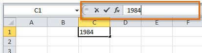
Formula Bar
In the formula bar, you can enter or edit data, a formula, or a function that will appear in a specific cell. In this image, cell C1 is selected and 1984 is entered into the formula bar. Note how the data appears in both the formula bar and in cell C1.
Column
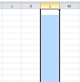
A column is a group of cells that runs from the top of the page to the bottom. In Excel, columns are identified by letters. Column L is selected here.
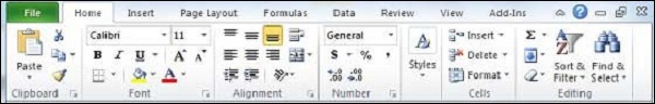
Ribbon
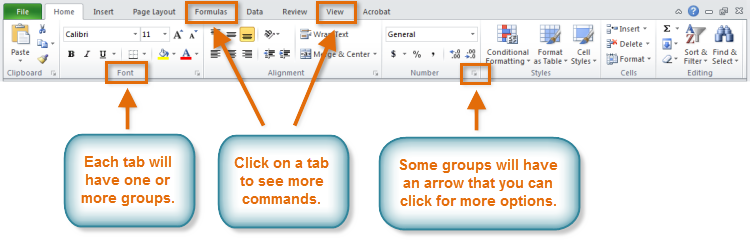
The Ribbon contains all of the commands you will need in order to perform common tasks. It has multiple tabs, each with several groups of commands, and you can add your own tabs that contain your favorite commands. Some groups have an arrow in the bottom-right corner that you can click to see even more options.
Working with your Excel environment
The Ribbon and Quick Access toolbar are where you’ll find the commands you need to perform common tasks in Excel. If you are familiar with Excel 2007, you will find that the main difference in the Excel 2010 Ribbon is that commands such as Open and Print are now housed in Backstage view.
The Ribbon
The Ribbon contains multiple tabs, each with several groups of commands. You can add your own tabs that contain your favorite commands.
Certain programs—such as Adobe Acrobat Reader—may install additional tabs to the Ribbon. These tabs are called add-ins.
To customize the Ribbon:
You can customize the Ribbon by creating your own tabs that house your desired commands. Commands are always housed within a group, and you can create as many groups as you need to keep your tabs organized. You can also add commands to any of the default tabs as long as you create a custom group within the tab.
- Right-click the Ribbon, then select Customize the Ribbon. A dialog box will appear.
If you do not see the command you want, click the Choose commands drop-down box and select All Commands.
To minimize and maximize the Ribbon:
The Ribbon is designed to be easy to use and responsive to your current tasks; however, if you find that it’s taking up too much of your screen space, you can minimize it.
- Click the arrow in the upper-right corner of the Ribbon to minimize it.
When the Ribbon is minimized, you can make it reappear by clicking a tab. However, the Ribbon will disappear again when you’re not using it.
The Quick Access toolbar
The Quick Access toolbar, above the Ribbon, lets you access common commands no matter which tab you are on. By default, it shows the Save, Undo, and Repeat commands. You can add other commands to make it more convenient for you.
To add commands to the Quick Access toolbar:
- Click the drop-down arrow to the right of the Quick Access toolbar.
- Select the command you want to add from the drop-down menu. To choose from more commands, select More Commands.
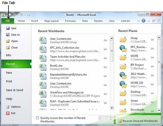
Backstage view
Backstage view gives you various options for saving, opening a file, printing, and sharing your document. It is similar to the Microsoft Office button menu from Excel 2007 and the File menu from earlier versions of Excel. However, instead of just a menu it’s a full-page view, which makes it easier to work with.
To get to Backstage view:
- On the Ribbon, click the File tab.
Click the buttons in the interactive below to learn about the different things you can do in Backstage view.
Options
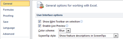
Here, you can change various Excel options. For example, you can control the spelling and grammar check settings, AutoRecover settings, and Language preferences.
From here, you can access Microsoft Office Help or check for updates.
Save & Send
Save & Send makes it easy to email your workbook, post it online, or change the file format.
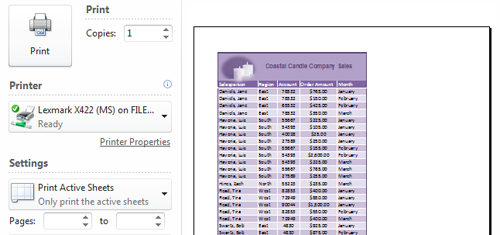
From the Print pane, you can change the print settings and print your workbook. You can also see a preview of your workbook.
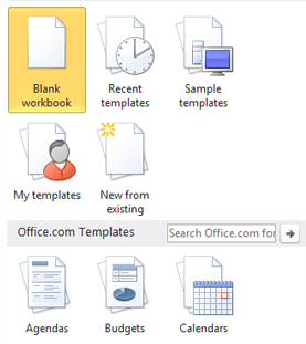
From here, you can create a new blank workbook, or you can choose from a large selection of templates.
Save, Save As, Open, and Close
Familiar tasks such as Save, Save As, Open, and Close are now found in Backstage view.
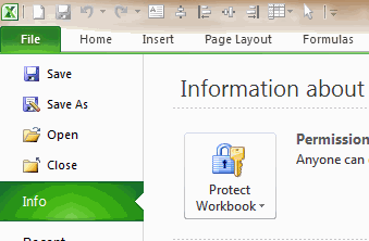
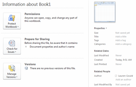
Info contains information about the current workbook. You can also inspect and edit its permissions.
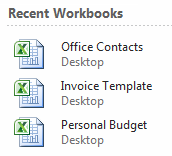
Recent
For convenience, recent workbooks will appear here.
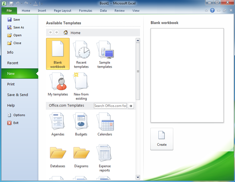
Creating and opening workbooks
Excel files are called workbooks. Each workbook holds one or more worksheets (also known as spreadsheets).
To create a new blank workbook:
- Click the File tab. This takes you to Backstage view.
- Select New.
- Select Blank workbook under Available Templates. It will be highlighted by default.
- Click Create. A new blank workbook appears in the Excel window.
To save time, you can create your document from a template, which you can select under Available Templates. We’ll talk more about this in a later lesson.
To open an existing workbook:
- Click the File tab. This takes you to Backstage view.
- Select Open. The Open dialog box appears.
If you have opened the existing workbook recently, it may be easier to choose Recent from the File tab instead of Open to search for your workbook.
Compatibility mode
Sometimes you may need to work with workbooks that were created in earlier versions of Microsoft Excel, such as Excel 2003 or Excel 2000. When you open these types of workbooks, they will appear in Compatibility mode.
Compatibility mode disables certain features, so you’ll only be able to access commands found in the program that was used to create the workbook. For example, if you open a workbook created in Excel 2003 you can only use tabs and commands found in Excel 2003.
In the image below, the workbook has opened in Compatibility mode. You can see that the sparklines and slicers features have been disabled.
To exit Compatibility mode, you’ll need to convert the workbook to the current version type. However, if you’re collaborating with others who only have access to an earlier version of Excel, it’s best to leave the workbook in Compatibility mode so the format will not change.
To convert a workbook:
If you want access to all of the Excel 2010 features, you can convert the workbook to the 2010 file format.
Note that converting a file may cause some changes to the original layout of the workbook.
- Click the File tab to access Backstage view.
- Locate and select the Convert command.
Источник
Getting Started with Excel 2010
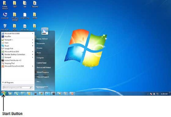
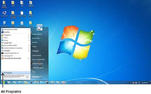
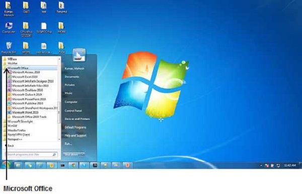
This chapter teaches you how to start an excel 2010 application in simple steps. Assuming you have Microsoft Office 2010 installed in your PC, start the excel application following the below mentioned steps in your PC.
Step 1 − Click on the Start button.
Step 2 − Click on All Programs option from the menu.
Step 3 − Search for Microsoft Office from the sub menu and click it.
Step 4 − Search for Microsoft Excel 2010 from the submenu and click it.
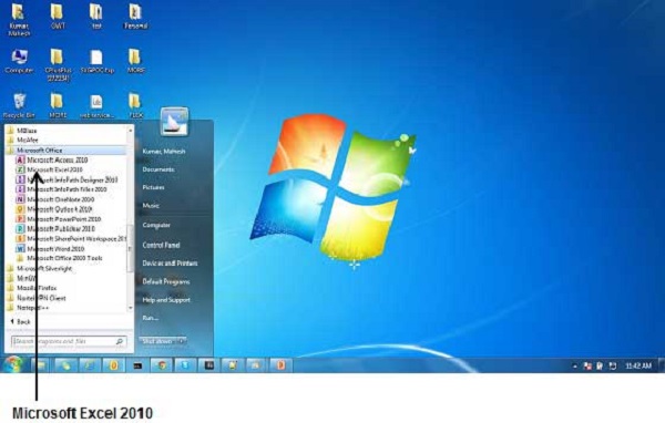
This will launch the Microsoft Excel 2010 application and you will see the following excel window.
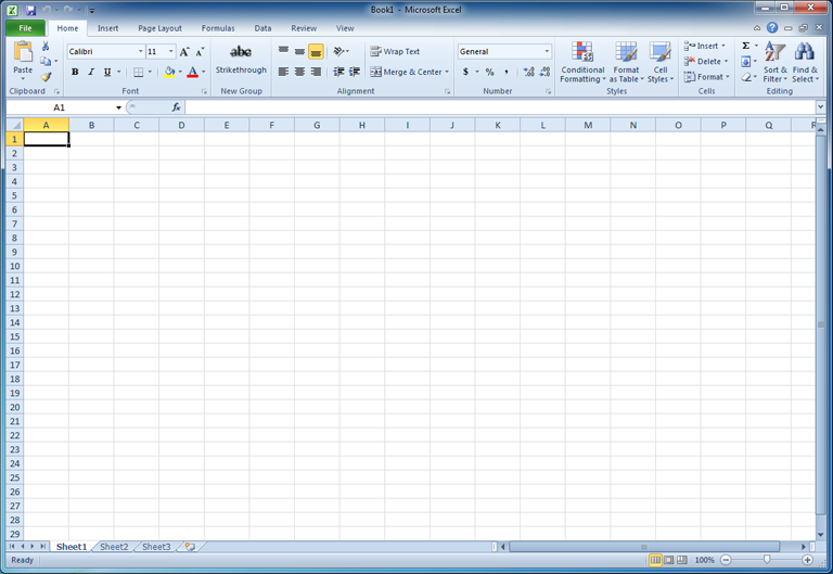
Explore Window in Excel 2010
The following basic window appears when you start the excel application. Let us now understand the various important parts of this window.
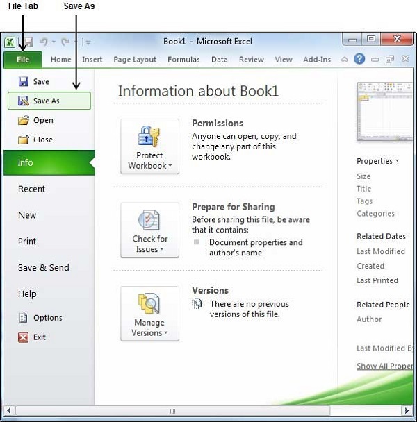
File Tab
The File tab replaces the Office button from Excel 2007. You can click it to check the Backstage view, where you come when you need to open or save files, create new sheets, print a sheet, and do other file-related operations.
Quick Access Toolbar
You will find this toolbar just above the File tab and its purpose is to provide a convenient resting place for the Excel’s most frequently used commands. You can customize this toolbar based on your comfort.
Ribbon
Ribbon contains commands organized in three components −
-
Tabs − They appear across the top of the Ribbon and contain groups of related commands. Home, Insert, Page Layout are the examples of ribbon tabs.
-
Groups − They organize related commands; each group name appears below the group on the Ribbon. For example, group of commands related to fonts or group of commands related to alignment etc.
-
Commands − Commands appear within each group as mentioned above.
Title Bar
This lies in the middle and at the top of the window. Title bar shows the program and the sheet titles.
Help
The Help Icon can be used to get excel related help anytime you like. This provides nice tutorial on various subjects related to excel.
Zoom Control
Zoom control lets you zoom in for a closer look at your text. The zoom control consists of a slider that you can slide left or right to zoom in or out. The + buttons can be clicked to increase or decrease the zoom factor.
View Buttons
The group of three buttons located to the left of the Zoom control, near the bottom of the screen, lets you switch among excel’s various sheet views.
-
Normal Layout view − This displays the page in normal view.
-
Page Layout view − This displays pages exactly as they will appear when printed. This gives a full screen look of the document.
-
Page Break view − This shows a preview of where pages will break when printed.
Sheet Area
The area where you enter data. The flashing vertical bar is called the insertion point and it represents the location where text will appear when you type.
Row Bar
Rows are numbered from 1 onwards and keeps on increasing as you keep entering data. Maximum limit is 1,048,576 rows.
Column Bar
Columns are numbered from A onwards and keeps on increasing as you keep entering data. After Z, it will start the series of AA, AB and so on. Maximum limit is 16,384 columns.
Status Bar
This displays the current status of the active cell in the worksheet. A cell can be in either of the fours states (a) Ready mode which indicates that the worksheet is ready to accept user inpu (b) Edit mode indicates that cell is editing mode, if it is not activated the you can activate editing mode by double-clicking on a cell (c) A cell enters into Enter mode when a user types data into a cell (d) Point mode triggers when a formula is being entered using a cell reference by mouse pointing or the arrow keys on the keyboard.
Dialog Box Launcher
This appears as a very small arrow in the lower-right corner of many groups on the Ribbon. Clicking this button opens a dialog box or task pane that provides more options about the group.
BackStage View in Excel 2010
The Backstage view has been introduced in Excel 2010 and acts as the central place for managing your sheets. The backstage view helps in creating new sheets, saving and opening sheets, printing and sharing sheets, and so on.
Getting to the Backstage View is easy. Just click the File tab located in the upper-left corner of the Excel Ribbon. If you already do not have any opened sheet then you will see a window listing down all the recently opened sheets as follows −
If you already have an opened sheet then it will display a window showing the details about the opened sheet as shown below. Backstage view shows three columns when you select most of the available options in the first column.
First column of the backstage view will have the following options −
| S.No. | Option & Description |
|---|---|
| 1 |
Save If an existing sheet is opened, it would be saved as is, otherwise it will display a dialogue box asking for the sheet name. |
| 2 |
Save As A dialogue box will be displayed asking for sheet name and sheet type. By default, it will save in sheet 2010 format with extension .xlsx. |
| 3 |
Open This option is used to open an existing excel sheet. |
| 4 |
Close This option is used to close an opened sheet. |
| 5 |
Info This option displays the information about the opened sheet. |
| 6 |
Recent This option lists down all the recently opened sheets. |
| 7 |
New This option is used to open a new sheet. |
| 8 |
This option is used to print an opened sheet. |
| 9 |
Save & Send This option saves an opened sheet and displays options to send the sheet using email etc. |
| 10 |
Help You can use this option to get the required help about excel 2010. |
| 11 |
Options Use this option to set various option related to excel 2010. |
| 12 |
Exit Use this option to close the sheet and exit. |
Sheet Information
When you click Info option available in the first column, it displays the following information in the second column of the backstage view −
-
Compatibility Mode − If the sheet is not a native excel 2007/2010 sheet, a Convert button appears here, enabling you to easily update its format. Otherwise, this category does not appear.
-
Permissions − You can use this option to protect the excel sheet. You can set a password so that nobody can open your sheet, or you can lock the sheet so that nobody can edit your sheet.
-
Prepare for Sharing − This section highlights important information you should know about your sheet before you send it to others, such as a record of the edits you made as you developed the sheet.
-
Versions − If the sheet has been saved several times, you may be able to access previous versions of it from this section.
Sheet Properties
When you click Info option available in the first column, it displays various properties in the third column of the backstage view. These properties include sheet size, title, tags, categories etc.
You can also edit various properties. Just try to click on the property value and if property is editable, then it will display a text box where you can add your text like title, tags, comments, Author.
Exit Backstage View
It is simple to exit from the Backstage View. Either click on the File tab or press the Esc button on the keyboard to go back to excel working mode.
Entering Values in Excel 2010
Entering values in excel sheet is a child’s play and this chapter shows how to enter values in an excel sheet. A new sheet is displayed by default when you open an excel sheet as shown in the below screen shot.
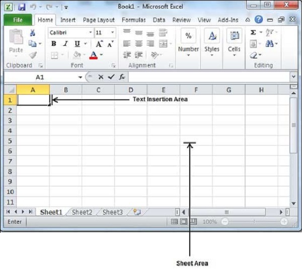
Sheet area is the place where you type your text. The flashing vertical bar is called the insertion point and it represents the location where text will appear when you type. When you click on a box then the box is highlighted. When you double click the box, the flashing vertical bar appears and you can start entering your data.
So, just keep your mouse cursor at the text insertion point and start typing whatever text you would like to type. We have typed only two words «Hello Excel» as shown below. The text appears to the left of the insertion point as you type.
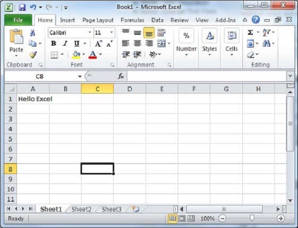
There are following three important points, which would help you while typing −
- Press Tab to go to next column.
- Press Enter to go to next row.
- Press Alt + Enter to enter a new line in the same column.
Move Around in Excel 2010
Excel provides a number of ways to move around a sheet using the mouse and the keyboard.
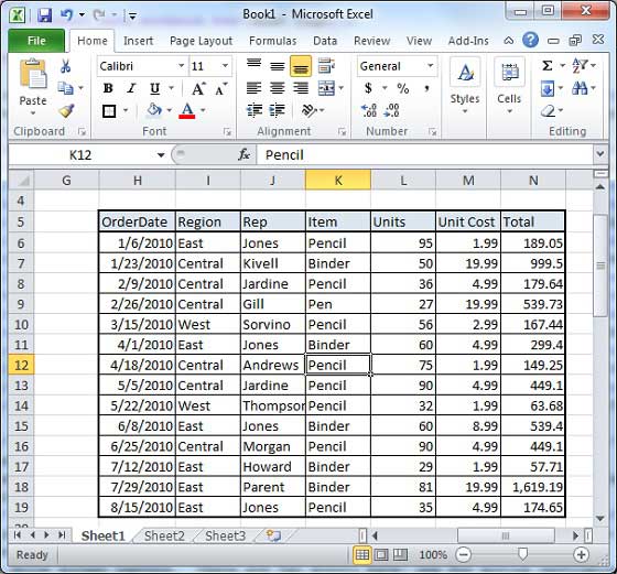
First of all, let us create some sample text before we proceed. Open a new excel sheet and type any data. We’ve shown a sample data in the screenshot.
| OrderDate | Region | Rep | Item | Units | Unit Cost | Total |
|---|---|---|---|---|---|---|
| 1/6/2010 | East | Jones | Pencil | 95 | 1.99 | 189.05 |
| 1/23/2010 | Central | Kivell | Binder | 50 | 19.99 | 999.5 |
| 2/9/2010 | Central | Jardine | Pencil | 36 | 4.99 | 179.64 |
| 2/26/2010 | Central | Gill | Pen | 27 | 19.99 | 539.73 |
| 3/15/2010 | West | Sorvino | Pencil | 56 | 2.99 | 167.44 |
| 4/1/2010 | East | Jones | Binder | 60 | 4.99 | 299.4 |
| 4/18/2010 | Central | Andrews | Pencil | 75 | 1.99 | 149.25 |
| 5/5/2010 | Central | Jardine | Pencil | 90 | 4.99 | 449.1 |
| 5/22/2010 | West | Thompson | Pencil | 32 | 1.99 | 63.68 |
| 6/8/2010 | East | Jones | Binder | 60 | 8.99 | 539.4 |
| 6/25/2010 | Central | Morgan | Pencil | 90 | 4.99 | 449.1 |
| 7/12/2010 | East | Howard | Binder | 29 | 1.99 | 57.71 |
| 7/29/2010 | East | Parent | Binder | 81 | 19.99 | 1,619.19 |
| 8/15/2010 | East | Jones | Pencil | 35 | 4.99 | 174.65 |
Moving with Mouse
You can easily move the insertion point by clicking in your text anywhere on the screen. Sometime if the sheet is big then you cannot see a place where you want to move. In such situations, you would have to use the scroll bars, as shown in the following screen shot −
You can scroll your sheet by rolling your mouse wheel, which is equivalent to clicking the up-arrow or down-arrow buttons in the scroll bar.
Moving with Scroll Bars
As shown in the above screen capture, there are two scroll bars: one for moving vertically within the sheet, and one for moving horizontally. Using the vertical scroll bar, you may −
-
Move upward by one line by clicking the upward-pointing scroll arrow.
-
Move downward by one line by clicking the downward-pointing scroll arrow.
-
Move one next page, using next page button (footnote).
-
Move one previous page, using previous page button (footnote).
-
Use Browse Object button to move through the sheet, going from one chosen object to the next.
Moving with Keyboard
The following keyboard commands, used for moving around your sheet, also move the insertion point −
| Keystroke | Where the Insertion Point Moves |
|---|---|
 |
Forward one box |
 |
Back one box |
 |
Up one box |
 |
Down one box |
| PageUp | To the previous screen |
| PageDown | To the next screen |
| Home | To the beginning of the current screen |
| End | To the end of the current screen |
You can move box by box or sheet by sheet. Now click in any box containing data in the sheet. You would have to hold down the Ctrl key while pressing an arrow key, which moves the insertion point as described here −
| Key Combination | Where the Insertion Point Moves |
|---|---|
| Ctrl + |
To the last box containing data of the current row. |
| Ctrl + |
To the first box containing data of the current row. |
| Ctrl + |
To the first box containing data of the current column. |
| Ctrl + |
To the last box containing data of the current column. |
| Ctrl + PageUp | To the sheet in the left of the current sheet. |
| Ctrl + PageDown | To the sheet in the right of the current sheet. |
| Ctrl + Home | To the beginning of the sheet. |
| Ctrl + End | To the end of the sheet. |
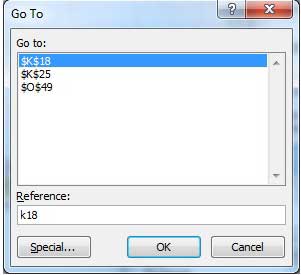
Moving with Go To Command
Press F5 key to use Go To command, which will display a dialogue box where you will find various options to reach to a particular box.
Normally, we use row and column number, for example K5 and finally press Go To button.
Save Workbook in Excel 2010
Saving New Sheet
Once you are done with typing in your new excel sheet, it is time to save your sheet/workbook to avoid losing work you have done on an Excel sheet. Following are the steps to save an edited excel sheet −
Step 1 − Click the File tab and select Save As option.
Step 2 − Select a folder where you would like to save the sheet, Enter file name, which you want to give to your sheet and Select a Save as type, by default it is .xlsx format.
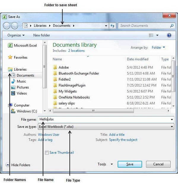
Step 3 − Finally, click on Save button and your sheet will be saved with the entered name in the selected folder.
Saving New Changes
There may be a situation when you open an existing sheet and edit it partially or completely, or even you would like to save the changes in between editing of the sheet. If you want to save this sheet with the same name, then you can use either of the following simple options −
-
Just press Ctrl + S keys to save the changes.
-
Optionally, you can click on the floppy icon available at the top left corner and just above the File tab. This option will also save the changes.
-
You can also use third method to save the changes, which is the Save option available just above the Save As option as shown in the above screen capture.
If your sheet is new and it was never saved so far, then with either of the three options, word would display you a dialogue box to let you select a folder, and enter sheet name as explained in case of saving new sheet.
Create Worksheet in Excel 2010
Creating New Worksheet
Three new blank sheets always open when you start Microsoft Excel. Below steps explain you how to create a new worksheet if you want to start another new worksheet while you are working on a worksheet, or you closed an already opened worksheet and want to start a new worksheet.
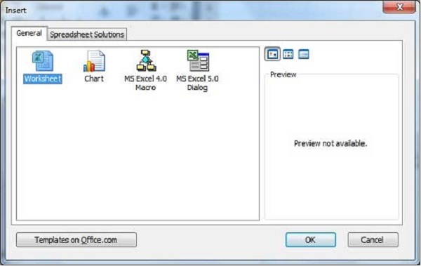
Step 1 − Right Click the Sheet Name and select Insert option.
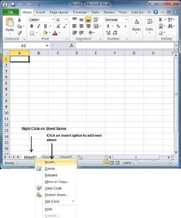
Step 2 − Now you’ll see the Insert dialog with select Worksheet option as selected from the general tab. Click the Ok button.
Now you should have your blank sheet as shown below ready to start typing your text.
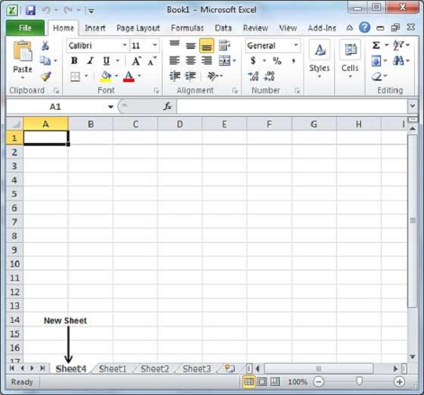
You can use a short cut to create a blank sheet anytime. Try using the Shift+F11 keys and you will see a new blank sheet similar to the above sheet is opened.
Copy Worksheet in Excel 2010
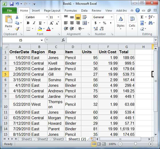
Copy Worksheet
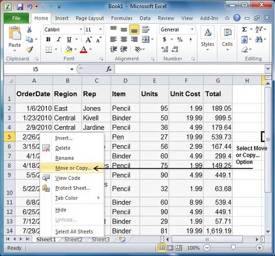
First of all, let us create some sample text before we proceed. Open a new excel sheet and type any data. We’ve shown a sample data in the screenshot.
| OrderDate | Region | Rep | Item | Units | Unit Cost | Total |
|---|---|---|---|---|---|---|
| 1/6/2010 | East | Jones | Pencil | 95 | 1.99 | 189.05 |
| 1/23/2010 | Central | Kivell | Binder | 50 | 19.99 | 999.5 |
| 2/9/2010 | Central | Jardine | Pencil | 36 | 4.99 | 179.64 |
| 2/26/2010 | Central | Gill | Pen | 27 | 19.99 | 539.73 |
| 3/15/2010 | West | Sorvino | Pencil | 56 | 2.99 | 167.44 |
| 4/1/2010 | East | Jones | Binder | 60 | 4.99 | 299.4 |
| 4/18/2010 | Central | Andrews | Pencil | 75 | 1.99 | 149.25 |
| 5/5/2010 | Central | Jardine | Pencil | 90 | 4.99 | 449.1 |
| 5/22/2010 | West | Thompson | Pencil | 32 | 1.99 | 63.68 |
| 6/8/2010 | East | Jones | Binder | 60 | 8.99 | 539.4 |
| 6/25/2010 | Central | Morgan | Pencil | 90 | 4.99 | 449.1 |
| 7/12/2010 | East | Howard | Binder | 29 | 1.99 | 57.71 |
| 7/29/2010 | East | Parent | Binder | 81 | 19.99 | 1,619.19 |
| 8/15/2010 | East | Jones | Pencil | 35 | 4.99 | 174.65 |
Here are the steps to copy an entire worksheet.
Step 1 − Right Click the Sheet Name and select the Move or Copy option.
Step 2 − Now you’ll see the Move or Copy dialog with select Worksheet option as selected from the general tab. Click the Ok button.
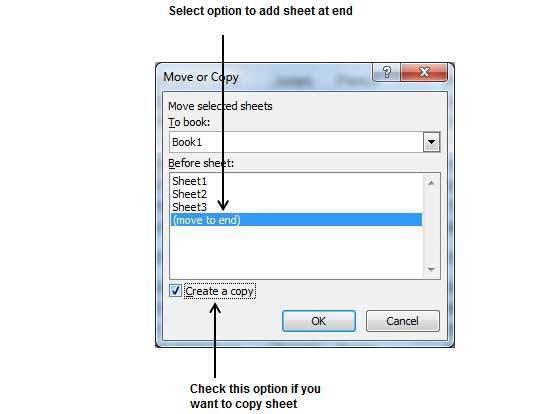
Select Create a Copy Checkbox to create a copy of the current sheet and Before sheet option as (move to end) so that new sheet gets created at the end.
Press the Ok Button.
Now you should have your copied sheet as shown below.
You can rename the sheet by double clicking on it. On double click, the sheet name becomes editable. Enter any name say Sheet5 and press Tab or Enter Key.
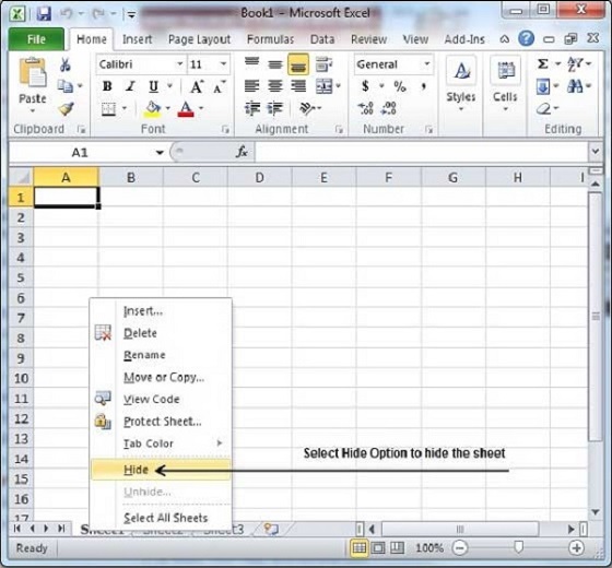
Hiding Worksheet in Excel 2010
Hiding Worksheet
Here is the step to hide a worksheet.
Step − Right Click the Sheet Name and select the Hide option. Sheet will get hidden.
Unhiding Worksheet
Here are the steps to unhide a worksheet.
Step 1 − Right Click on any Sheet Name and select the Unhide… option.
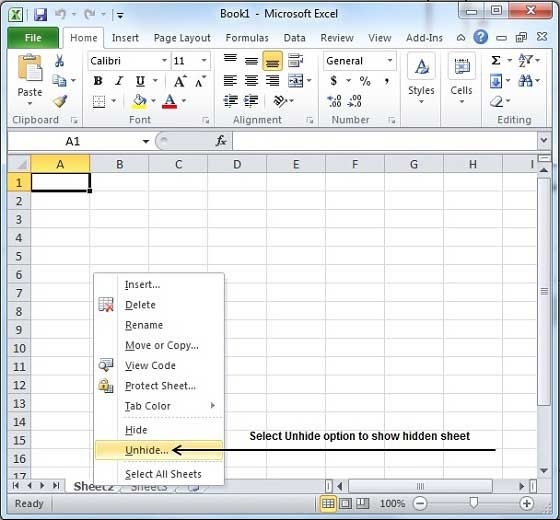
Step 2 − Select Sheet Name to unhide in Unhide dialog to unhide the sheet.
Press the Ok Button.
Now you will have your hidden sheet back.
Delete Worksheet in Excel 2010
Delete Worksheet
Here is the step to delete a worksheet.
Step − Right Click the Sheet Name and select the Delete option.
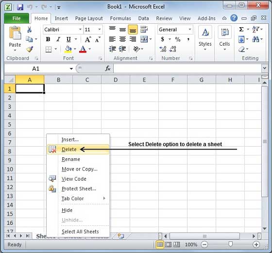
Sheet will get deleted if it is empty, otherwise you’ll see a confirmation message.
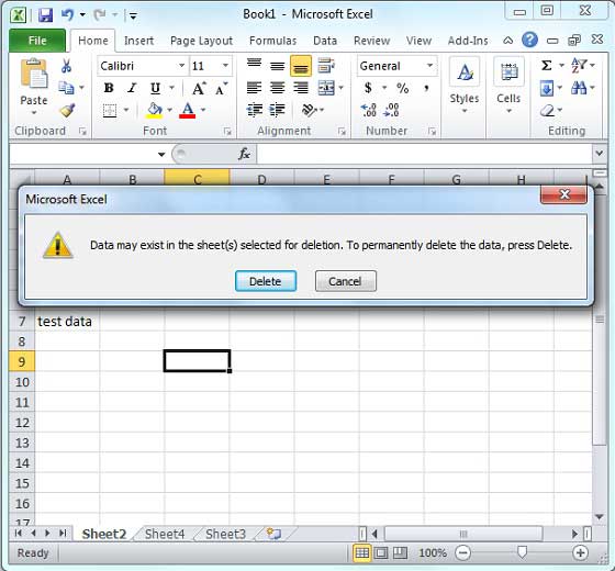
Press the Delete Button.
Now your worksheet will get deleted.
Close Workbook in Excel 2010
Close Workbook
Here are the steps to close a workbook.
Step 1 − Click the Close Button as shown below.
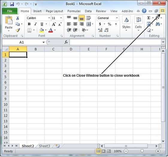
You’ll see a confirmation message to save the workbook.
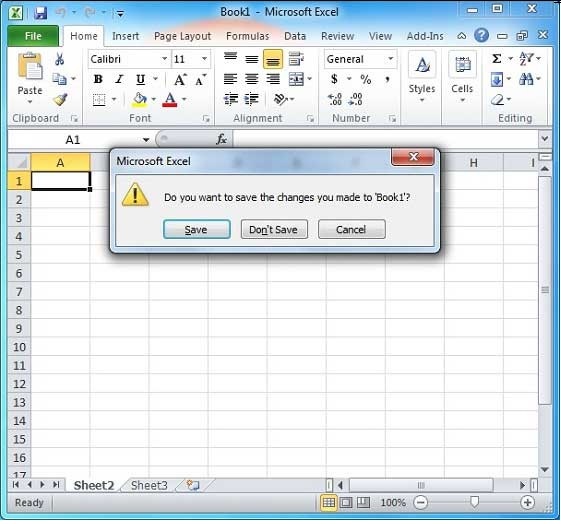
Step 2 − Press the Save Button to save the workbook as we did in MS Excel — Save Workbook chapter.
Now your worksheet will get closed.
Open Workbook in Excel 2010
Let us see how to open workbook from excel in the below mentioned steps.
Step 1 − Click the File Menu as shown below. You can see the Open option in File Menu.
There are two more columns Recent workbooks and Recent places, where you can see the recently opened workbooks and the recent places from where workbooks are opened.
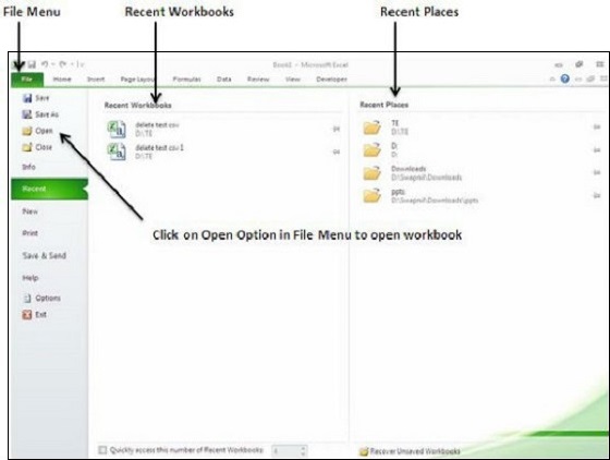
Step 2 − Clicking the Open Option will open the browse dialog as shown below. Browse the directory and find the file you need to open.
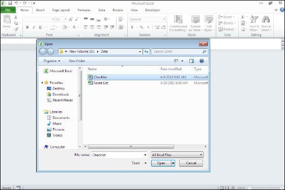
Step 3 − Once you select the workbook your workbook will be opened as below −

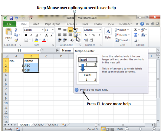
Context Help in Excel 2010
MS Excel provides context sensitive help on mouse over. To see context sensitive help for a particular Menu option, hover the mouse over the option for some time. Then you can see the context sensitive Help as shown below.
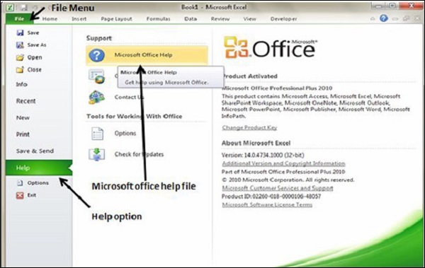
Getting More Help
For getting more help with MS Excel from Microsoft you can press F1 or by File → Help → Support → Microsoft Office Help.
Insert Data in Excel 2010
In MS Excel, there are 1048576*16384 cells. MS Excel cell can have Text, Numeric value or formulas. An MS Excel cell can have maximum of 32000 characters.
Inserting Data
For inserting data in MS Excel, just activate the cell type text or number and press enter or Navigation keys.
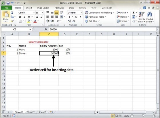
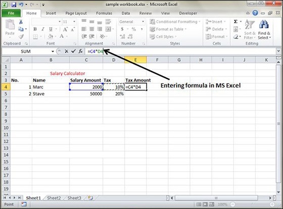
Inserting Formula
For inserting formula in MS Excel go to the formula bar, enter the formula and then press enter or navigation key. See the screen-shot below to understand it.
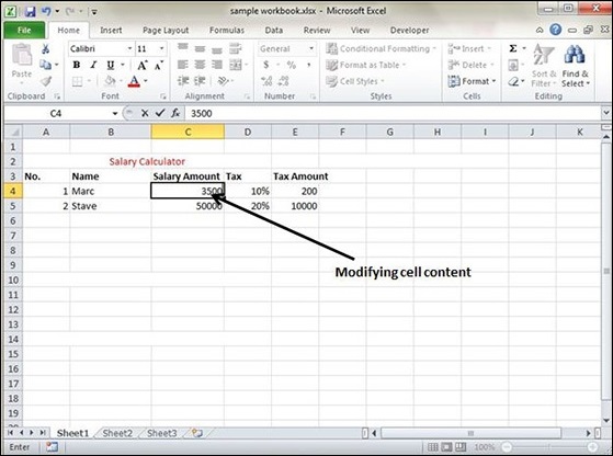
Modifying Cell Content
For modifying the cell content just activate the cell, enter a new value and then press enter or navigation key to see the changes. See the screen-shot below to understand it.
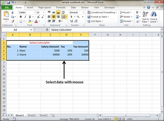
Select Data in Excel 2010
MS Excel provides various ways of selecting data in the sheet. Let us see those ways.
Select with Mouse
Drag the mouse over the data you want to select. It will select those cells as shown below.
Select with Special
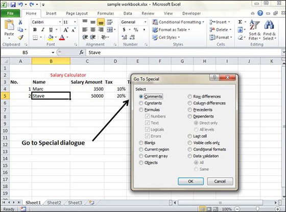
If you want to select specific region, select any cell in that region. Pressing F5 will show the below dialogue box.
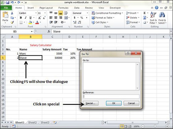
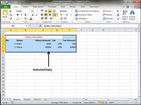
Click on Special button to see the below dialogue box. Select current region from the radio buttons. Click on ok to see the current region selected.
As you can see in the below screen, the data is selected for the current region.
Delete Data in Excel 2010
MS Excel provides various ways of deleting data in the sheet. Let us see those ways.
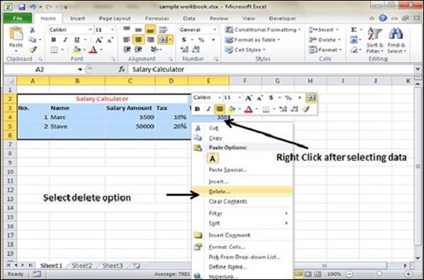
Delete with Mouse
Select the data you want to delete. Right Click on the sheet. Select the delete option, to delete the data.
Delete with Delete Key
Select the data you want to delete. Press on the Delete Button from the keyboard, it will delete the data.
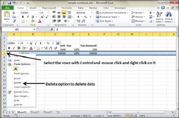
Selective Delete for Rows
Select the rows, which you want to delete with Mouse click + Control Key. Then right click to show the various options. Select the Delete option to delete the selected rows.
Move Data in Excel 2010
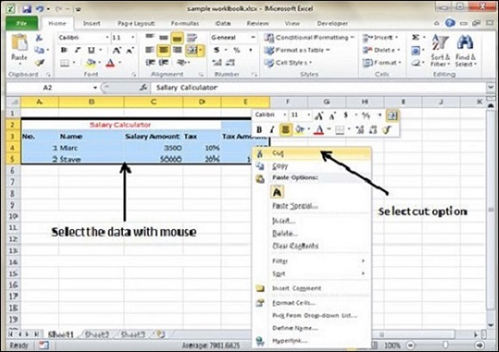
Let us see how we can Move Data with MS Excel.
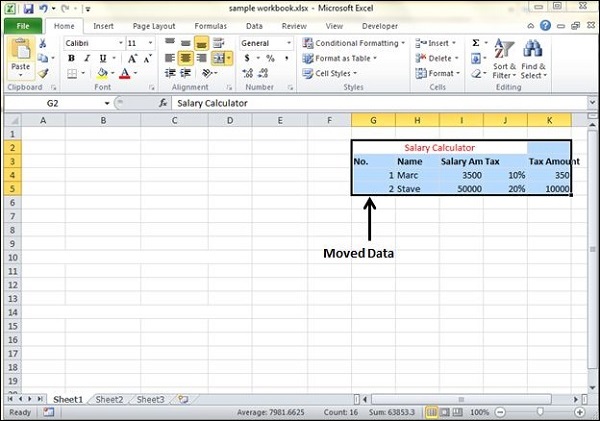
Step 1 − Select the data you want to Move. Right Click and Select the cut option.
Step 2 − Select the first cell where you want to move the data. Right click on it and paste the data. You can see the data is moved now.
Rows & Columns in Excel 2010
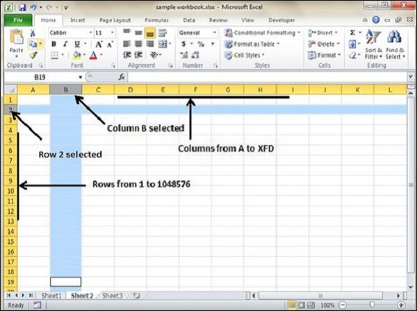
Row and Column Basics
MS Excel is in tabular format consisting of rows and columns.
-
Row runs horizontally while Column runs vertically.
-
Each row is identified by row number, which runs vertically at the left side of the sheet.
-
Each column is identified by column header, which runs horizontally at the top of the sheet.
For MS Excel 2010, Row numbers ranges from 1 to 1048576; in total 1048576 rows, and Columns ranges from A to XFD; in total 16384 columns.
Navigation with Rows and Columns
Let us see how to move to the last row or the last column.
-
You can go to the last row by clicking Control + Down Navigation arrow.
-
You can go to the last column by clicking Control + Right Navigation arrow.
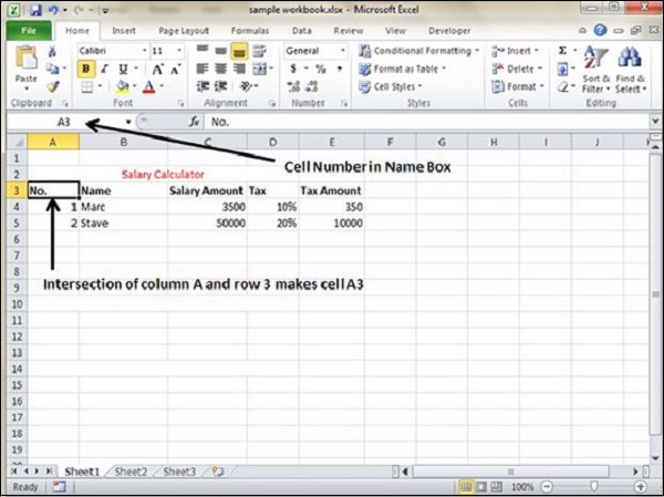
Cell Introduction
The intersection of rows and columns is called cell.
Cell is identified with Combination of column header and row number.
For example − A1, A2.
Copy & Paste in Excel 2010
MS Excel provides copy paste option in different ways. The simplest method of copy paste is as below.
Copy Paste
-
To copy and paste, just select the cells you want to copy. Choose copy option after right click or press Control + C.
-
Select the cell where you need to paste this copied content. Right click and select paste option or press Control + V.
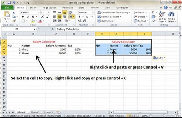
In this case, MS Excel will copy everything such as values, formulas, Formats, Comments and validation. MS Excel will overwrite the content with paste. If you want to undo this, press Control + Z from the keyboard.
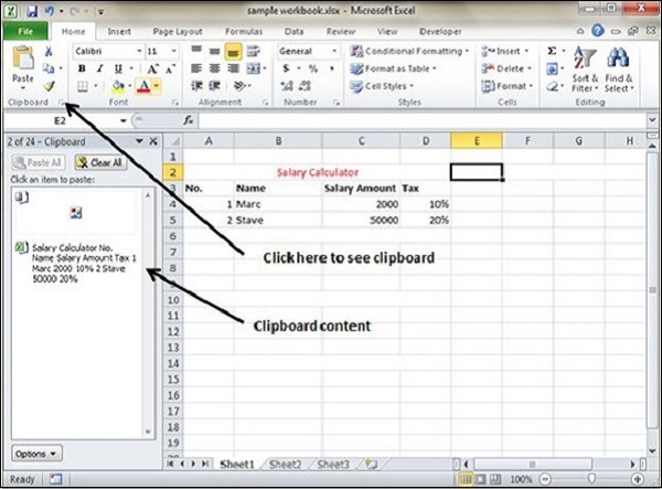
Copy Paste using Office Clipboard
When you copy data in MS Excel, it puts the copied content in Windows and Office Clipboard. You can view the clipboard content by Home → Clipboard. View the clipboard content. Select the cell where you need to paste. Click on paste, to paste the content.
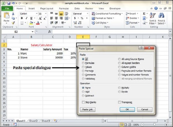
Copy Paste in Special way
You may not want to copy everything in some cases. For example, you want to copy only Values or you want to copy only the formatting of cells. Select the paste special option as shown below.
Below are the various options available in paste special.
-
All − Pastes the cell’s contents, formats, and data validation from the Windows Clipboard.
-
Formulas − Pastes formulas, but not formatting.
-
Values − Pastes only values not the formulas.
-
Formats − Pastes only the formatting of the source range.
-
Comments − Pastes the comments with the respective cells.
-
Validation − Pastes validation applied in the cells.
-
All using source theme − Pastes formulas, and all formatting.
-
All except borders − Pastes everything except borders that appear in the source range.
-
Column Width − Pastes formulas, and also duplicates the column width of the copied cells.
-
Formulas & Number Formats − Pastes formulas and number formatting only.
-
Values & Number Formats − Pastes the results of formulas, plus the number.
-
Merge Conditional Formatting − This icon is displayed only when the copied cells contain conditional formatting. When clicked, it merges the copied conditional formatting with any conditional formatting in the destination range.
-
Transpose − Changes the orientation of the copied range. Rows become columns, and columns become rows. Any formulas in the copied range are adjusted so that they work properly when transposed.
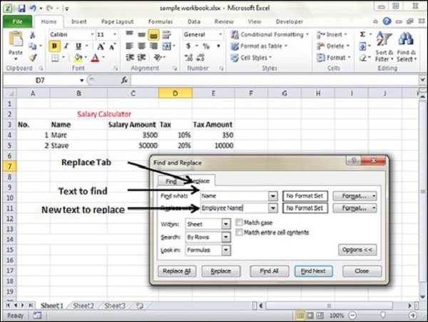
Find & Replace in Excel 2010
MS Excel provides Find & Replace option for finding text within the sheet.
Find and Replace Dialogue
Let us see how to access the Find & Replace Dialogue.
To access the Find & Replace, Choose Home → Find & Select → Find or press Control + F Key. See the image below.
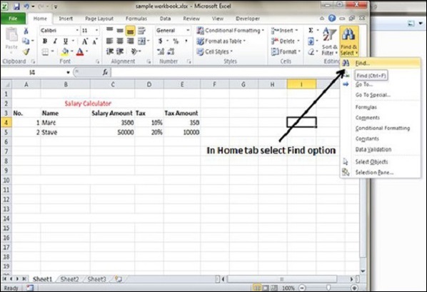
You can see the Find and Replace dialogue as below.
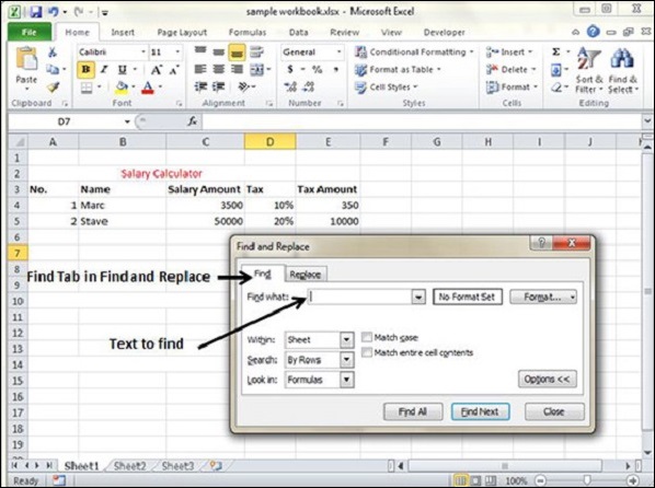
You can replace the found text with the new text in the Replace tab.
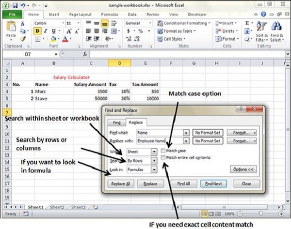
Exploring Options
Now, let us see the various options available under the Find dialogue.
-
Within − Specifying the search should be in Sheet or workbook.
-
Search By − Specifying the internal search method by rows or by columns.
-
Look In − If you want to find text in formula as well, then select this option.
-
Match Case − If you want to match the case like lower case or upper case of words, then check this option.
-
Match Entire Cell Content − If you want the exact match of the word with cell, then check this option.
Spell Check in Excel 2010
MS Excel provides a feature of Word Processing program called Spelling check. We can get rid of the spelling mistakes with the help of spelling check feature.
Spell Check Basis
Let us see how to access the spell check.
-
To access the spell checker, Choose Review ➪ Spelling or press F7.
-
To check the spelling in just a particular range, select the range before you activate the spell checker.
-
If the spell checker finds any words it does not recognize as correct, it displays the Spelling dialogue with suggested options.
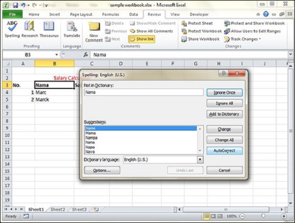
Exploring Options
Let us see the various options available in spell check dialogue.
-
Ignore Once − Ignores the word and continues the spell check.
-
Ignore All − Ignores the word and all subsequent occurrences of it.
-
Add to Dictionary − Adds the word to the dictionary.
-
Change − Changes the word to the selected word in the Suggestions list.
-
Change All − Changes the word to the selected word in the Suggestions list and changes all subsequent occurrences of it without asking.
-
AutoCorrect − Adds the misspelled word and its correct spelling (which you select from the list) to the AutoCorrect list.
Zoom In/Out in Excel 2010
Zoom Slider
By default, everything on screen is displayed at 100% in MS Excel. You can change the zoom percentage from 10% (tiny) to 400% (huge). Zooming doesn’t change the font size, so it has no effect on the printed output.
You can view the zoom slider at the right bottom of the workbook as shown below.
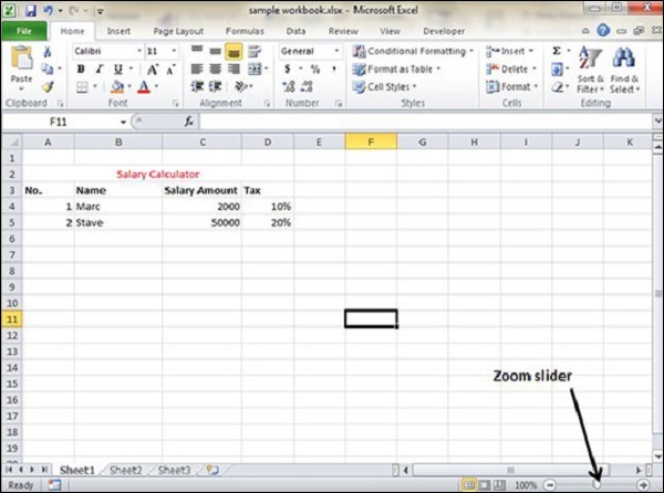
Zoom In
You can zoom in the workbook by moving the slider to the right. It will change the only view of the workbook. You can have maximum of 400% zoom in. See the below screen-shot.
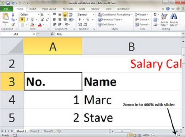
Zoom Out
You can zoom out the workbook by moving the slider to the left. It will change the only view of the workbook. You can have maximum of 10% zoom in. See the below screen-shot.
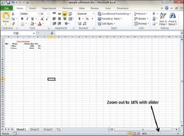
Special Symbols in Excel 2010
If you want to insert some symbols or special characters that are not found on the keyboard in that case you need to use the Symbols option.
Using Symbols
Go to Insert » Symbols » Symbol to view available symbols. You can see many symbols available there like Pi, alpha, beta, etc.
Select the symbol you want to add and click insert to use the symbol.
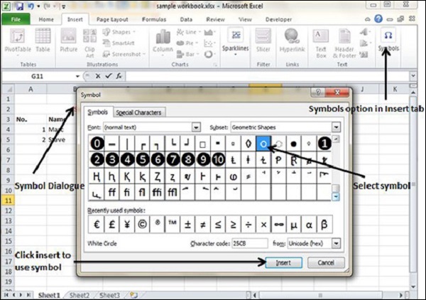
Using Special Characters
Go to Insert » Symbols » Special Characters to view the available special characters. You can see many special characters available there like Copyright, Registered etc.
Select the special character you want to add and click insert, to use the special character.
Insert Comments in Excel 2010
Adding Comment to Cell
Adding comment to cell helps in understanding the purpose of cell, what input it should have, etc. It helps in proper documentation.
To add comment to a cell, select the cell and perform any of the actions mentioned below.
- Choose Review » Comments » New Comment.
- Right-click the cell and choose Insert Comment from available options.
- Press Shift+F2.
Initially, a comment consists of Computer’s user name. You have to modify it with text for the cell comment.
Modifying Comment
You can modify the comment you have entered before as mentioned below.
- Select the cell on which the comment appears.
- Right-click the cell and choose the Edit Comment from the available options.
- Modify the comment.
Formatting Comment
Various formatting options are available for comments. For formatting a comment, Right click on cell » Edit comment » Select comment » Right click on it » Format comment. With formatting of comment you can change the color, font, size, etc of the comment.
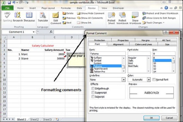
Add Text Box in Excel 2010
Text Boxes
Text boxes are special graphic objects that combine the text with a rectangular graphic object. Text boxes and cell comments are similar in displaying the text in rectangular box. But text boxes are always visible, while cell comments become visible after selecting the cell.
Adding Text Boxes
To add a text box, perform the below actions.
- Choose Insert » Text Box » choose text box or draw it.
Initially, the comment consists of Computer’s user name. You have to modify it with text for the cell comment.
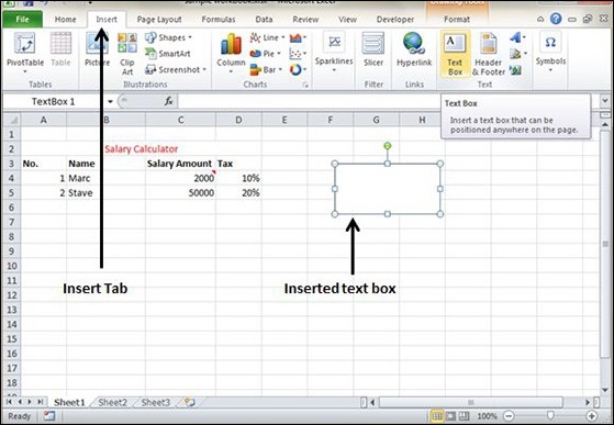
Formatting Text Box
After you have added the text box, you can format it by changing the font, font size, font style, and alignment, etc. Let us see some of the important options of formatting a text box.
-
Fill − Specifies the filling of text box like No fill, solid fill. Also specifying the transparency of text box fill.
-
Line Colour − Specifies the line colour and transparency of the line.
-
Line Style − Specifies the line style and width.
-
Size − Specifies the size of the text box.
-
Properties − Specifies some properties of the text box.
-
Text Box − Specifies text box layout, Auto-fit option and internal margins.
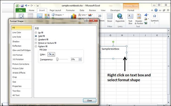
Undo Changes in Excel 2010
Undo Changes
You can reverse almost every action in Excel by using the Undo command. We can undo changes in following two ways.
- From the Quick access tool-bar » Click Undo.
- Press Control + Z.
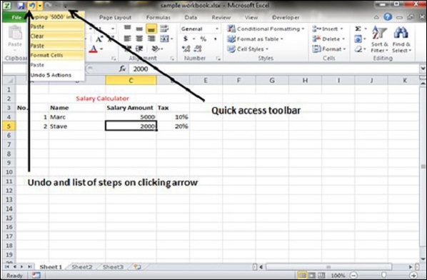
You can reverse the effects of the past 100 actions that you performed by executing Undo more than once. If you click the arrow on the right side of the Undo button, you see a list of the actions that you can reverse. Click an item in that list to undo that action and all the subsequent actions you performed.
Redo Changes
You can again reverse back the action done with undo in Excel by using the Redo command. We can redo changes in following two ways.
- From the Quick access tool-bar » Click Redo.
- Press Control + Y.
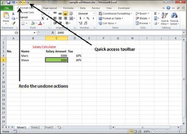
Setting Cell Type in Excel 2010
Formatting Cell
MS Excel Cell can hold different types of data like Numbers, Currency, Dates, etc. You can set the cell type in various ways as shown below −
- Right Click on the cell » Format cells » Number.
- Click on the Ribbon from the ribbon.
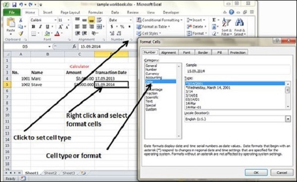
Various Cell Formats
Below are the various cell formats.
-
General − This is the default cell format of Cell.
-
Number − This displays cell as number with separator.
-
Currency − This displays cell as currency i.e. with currency sign.
-
Accounting − Similar to Currency, used for accounting purpose.
-
Date − Various date formats are available under this like 17-09-2013, 17th-Sep-2013, etc.
-
Time − Various Time formats are available under this, like 1.30PM, 13.30, etc.
-
Percentage − This displays cell as percentage with decimal places like 50.00%.
-
Fraction − This displays cell as fraction like 1/4, 1/2 etc.
-
Scientific − This displays cell as exponential like 5.6E+01.
-
Text − This displays cell as normal text.
-
Special − Special formats of cell like Zip code, Phone Number.
-
Custom − You can use custom format by using this.
Setting Fonts in Excel 2010
You can assign any of the fonts that is installed for your printer to cells in a worksheet.
Setting Font from Home
You can set the font of the selected text from Home » Font group » select the font.
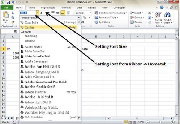
Setting Font From Format Cell Dialogue
- Right click on cell » Format cells » Font Tab
- Press Control + 1 or Shift + Control + F
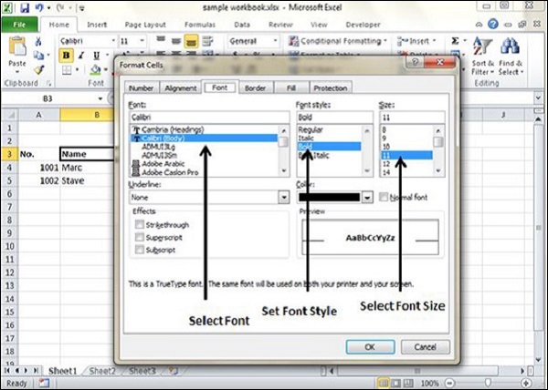
Text Decoration in Excel 2010
You can change the text decoration of the cell to change its look and feel.
Text Decoration
Various options are available in Home tab of the ribbon as mentioned below.
-
Bold − It makes the text in bold by choosing Home » Font Group » Click B or Press Control + B.
-
Italic − It makes the text italic by choosing Home » Font Group » Click I or Press Control + I.
-
Underline − It makes the text to be underlined by choosing Home » Font Group » Click U or Press Control + U.
-
Double Underline − It makes the text highlighted as double underlined by choose Home » Font Group » Click arrow near U » Select Double Underline.
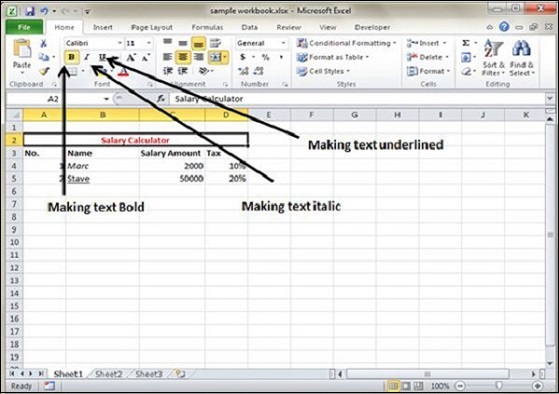
More Text Decoration Options
There are more options available for text decoration in Formatting cells » Font Tab »Effects cells as mentioned below.
-
Strike-through − It strikes the text in the center vertically.
-
Super Script − It makes the content to appear as a super script.
-
Sub Script − It makes content to appear as a sub script.
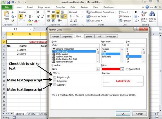
Rotate Cells in Excel 2010
You can rotate the cell by any degree to change the orientation of the cell.
Rotating Cell from Home Tab
Click on the orientation in the Home tab. Choose options available like Angle CounterClockwise, Angle Clockwise, etc.
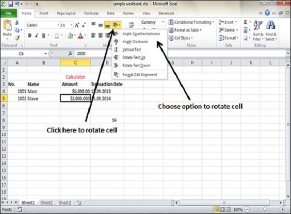
Rotating Cell from Formatting Cell
Right Click on the cell. Choose Format cells » Alignment » Set the degree for rotation.
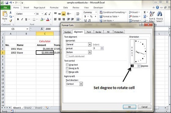
Setting Colors in Excel 2010
You can change the background color of the cell or text color.
Changing Background Color
By default the background color of the cell is white in MS Excel. You can change it as per your need from Home tab » Font group » Background color.
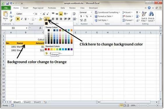
Changing Foreground Color
By default, the foreground or text color is black in MS Excel. You can change it as per your need from Home tab » Font group » Foreground color.
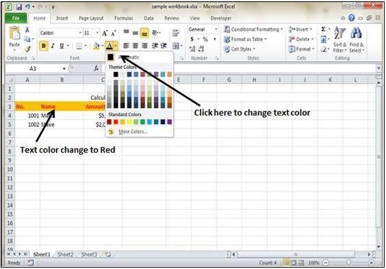
Also you can change the foreground color by selecting the cell Right click » Format cells » Font Tab » Color.
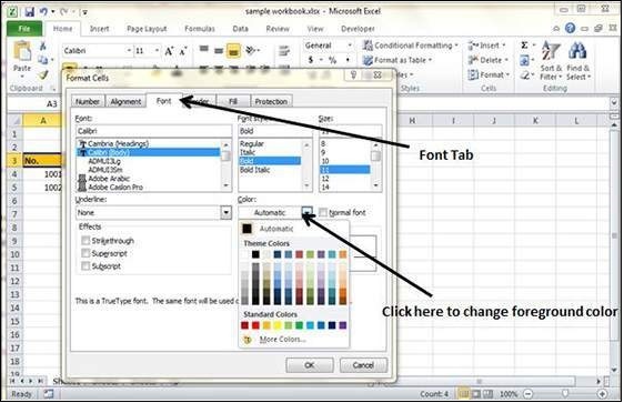
Text Alignments in Excel 2010
If you don’t like the default alignment of the cell, you can make changes in the alignment of the cell. Below are the various ways of doing it.
Change Alignment from Home Tab
You can change the Horizontal and vertical alignment of the cell. By default, Excel aligns numbers to the right and text to the left. Click on the available option in the Alignment group in Home tab to change alignment.
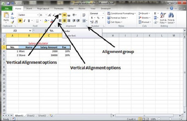
Change Alignment from Format Cells
Right click on the cell and choose format cell. In format cells dialogue, choose Alignment Tab. Select the available options from the Vertical alignment and Horizontal alignment options.
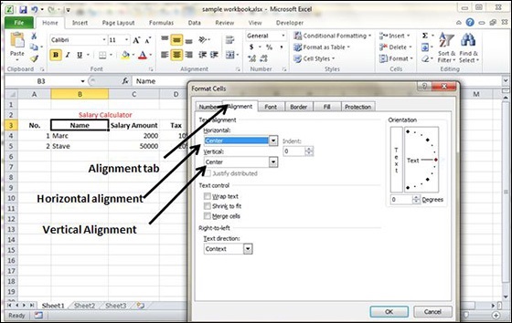
Exploring Alignment Options
1. Horizontal Alignment − You can set horizontal alignment to Left, Centre, Right, etc.
-
Left − Aligns the cell contents to the left side of the cell.
-
Center − Centers the cell contents in the cell.
-
Right − Aligns the cell contents to the right side of the cell.
-
Fill − Repeats the contents of the cell until the cell’s width is filled.
-
Justify − Justifies the text to the left and right of the cell. This option is applicable only if the cell is formatted as wrapped text and uses more than one line.
2. Vertical Alignment − You can set Vertical alignment to top, Middle, bottom, etc.
-
Top Aligns the cell contents to the top of the cell.
-
Center Centers the cell contents vertically in the cell.
-
Bottom Aligns the cell contents to the bottom of the cell.
-
Justify Justifies the text vertically in the cell; this option is applicable only if the cell is formatted as wrapped text and uses more than one line.
Merge & Wrap in Excel 2010
Merge Cells
MS Excel enables you to merge two or more cells. When you merge cells, you don’t combine the contents of the cells. Rather, you combine a group of cells into a single cell that occupies the same space.
You can merge cells by various ways as mentioned below.
-
Choose Merge & Center control on the Ribbon, which is simpler. To merge cells, select the cells that you want to merge and then click the Merge & Center button.
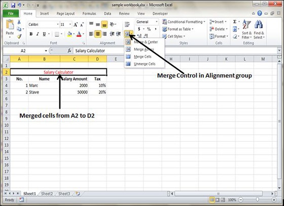
-
Choose Alignment tab of the Format Cells dialogue box to merge the cells.
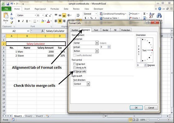
Additional Options
The Home » Alignment group » Merge & Center control contains a drop-down list with these additional options −
-
Merge Across − When a multi-row range is selected, this command creates multiple merged cells — one for each row.
-
Merge Cells − Merges the selected cells without applying the Center attribute.
-
Unmerge Cells − Unmerges the selected cells.
Wrap Text and Shrink to Fit
If the text is too wide to fit the column width but don’t want that text to spill over into adjacent cells, you can use either the Wrap Text option or the Shrink to Fit option to accommodate that text.
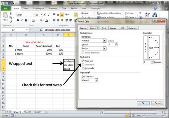
Borders and Shades in Excel 2010
Apply Borders
MS Excel enables you to apply borders to the cells. For applying border, select the range of cells Right Click » Format cells » Border Tab » Select the Border Style.
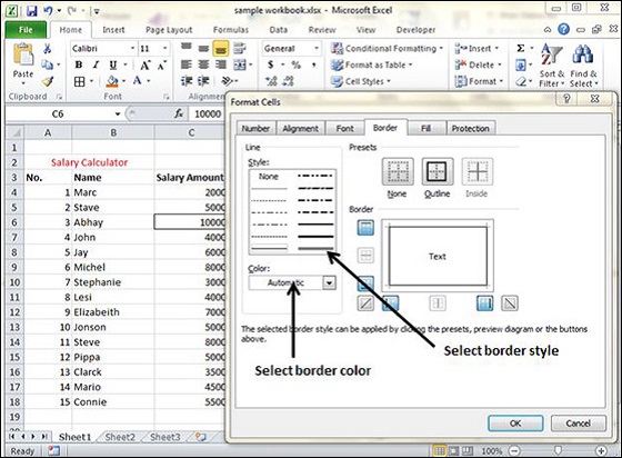
Then you can apply border by Home Tab » Font group »Apply Borders.
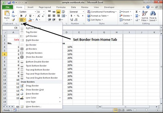
Apply Shading
You can add shading to the cell from the Home tab » Font Group » Select the Color.
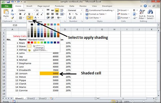
Apply Formatting in Excel 2010
Formatting Cells
In MS Excel, you can apply formatting to the cell or range of cells by Right Click » Format cells » Select the tab. Various tabs are available as shown below
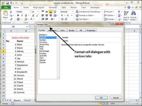
Alternative to Placing Background
-
Number − You can set the Format of the cell depending on the cell content. Find tutorial on this at MS Excel — Setting Cell Type.
-
Alignment − You can set the alignment of text on this tab. Find tutorial on this at MS Excel — Text Alignments.
-
Font − You can set the Font of text on this tab.Find tutorial on this at MS Excel — Setting Fonts.
-
Border − You can set border of cell with this tab.Find tutorial on this at MS Excel — Borders and Shades.
-
Fill − You can set fill of cell with this tab. Find tutorial on this at MS Excel — Borders and Shades.
-
Protection − You can set cell protection option with this tab.
Sheet Options in Excel 2010
Sheet Options
MS Excel provides various sheet options for printing purpose like generally cell gridlines aren’t printed. If you want your printout to include the gridlines, Choose Page Layout » Sheet Options group » Gridlines » Check Print.
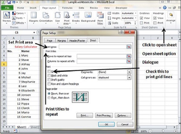
Options in Sheet Options Dialogue
-
Print Area − You can set the print area with this option.
-
Print Titles − You can set titles to appear at the top for rows and at the left for columns.
-
Print −
-
Gridlines − Gridlines to appear while printing worksheet.
-
Black & White − Select this check box to have your color printer print the chart in black and white.
-
Draft quality − Select this check box to print the chart using your printer’s draft-quality setting.
-
Rows & Column Heading − Select this check box to have rows and column heading to print.
-
-
Page Order −
-
Down, then Over − It prints the down pages first and then the right pages.
-
Over, then Down − It prints right pages first and then comes to print the down pages.
-
Adjust Margins in Excel 2010
Margins
Margins are the unprinted areas along the sides, top, and bottom of a printed page. All printed pages in MS Excel have the same margins. You can’t specify different margins for different pages.
You can set margins by various ways as explained below.
-
Choose Page Layout » Page Setup » Margins drop-down list, you can select Normal, Wide, Narrow, or the custom Setting.
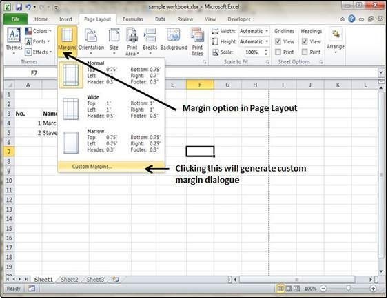
-
These options are also available when you choose File » Print.
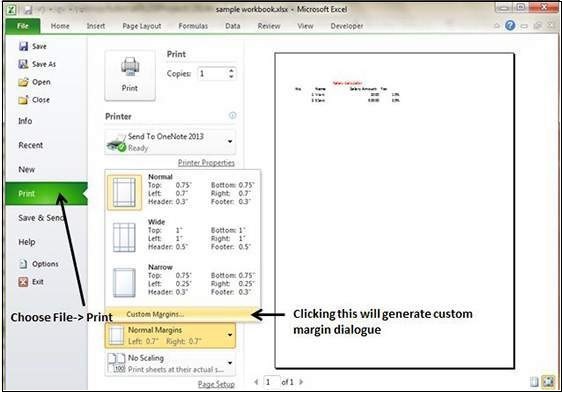
If none of these settings does the job, choose Custom Margins to display the Margins tab of the Page Setup dialog box, as shown below.
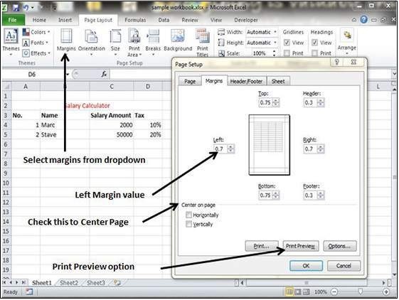
Center on Page
By default, Excel aligns the printed page at the top and left margins. If you want the output to be centered vertically or horizontally, select the appropriate check box in the Center on Page section of the Margins tab as shown in the above screenshot.
Page Orientation in Excel 2010
Page Orientation
Page orientation refers to how output is printed on the page. If you change the orientation, the onscreen page breaks adjust automatically to accommodate the new paper orientation.
Types of Page Orientation
-
Portrait − Portrait to print tall pages (the default).
-
Landscape − Landscape to print wide pages. Landscape orientation is useful when you have a wide range that doesn’t fit on a vertically oriented page.
Changing Page Orientation
-
Choose Page Layout » Page Setup » Orientation » Portrait or Landscape.
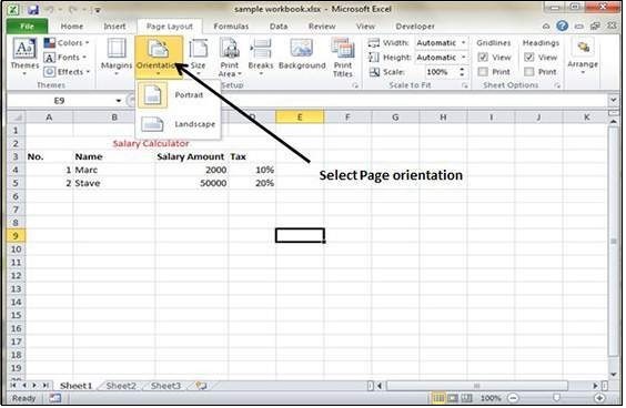
- Choose File » Print.
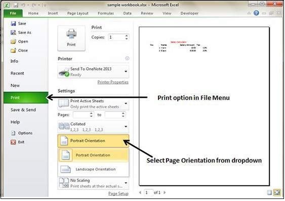
Header and Footer in Excel 2010
Header and Footer
A header is the information that appears at the top of each printed page and a footer is the information that appears at the bottom of each printed page. By default, new workbooks do not have headers or footers.
Adding Header and Footer
- Choose Page Setup dialog box » Header or Footer tab.
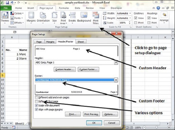
You can choose the predefined header and footer or create your custom ones.
-
&[Page] − Displays the page number.
-
&[Pages] − Displays the total number of pages to be printed.
-
&[Date] − Displays the current date.
-
&[Time] − Displays the current time.
-
&[Path]&[File] − Displays the workbook’s complete path and filename.
-
&[File] − Displays the workbook name.
-
&[Tab] − Displays the sheet’s name.
Other Header and Footer Options
When a header or footer is selected in Page Layout view, the Header & Footer » Design » Options group contains controls that let you specify other options −
-
Different First Page − Check this to specify a different header or footer for the first printed page.
-
Different Odd & Even Pages − Check this to specify a different header or footer for odd and even pages.
-
Scale with Document − If checked, the font size in the header and footer will be sized. Accordingly if the document is scaled when printed. This option is enabled, by default.
-
Align with Page Margins − If checked, the left header and footer will be aligned with the left margin, and the right header and footer will be aligned with the right margin. This option is enabled, by default.
Insert Page Break in Excel 2010
Page Breaks
If you don’t want a row to print on a page by itself or you don’t want a table header row to be the last line on a page. MS Excel gives you precise control over page breaks.
MS Excel handles page breaks automatically, but sometimes you may want to force a page break either a vertical or a horizontal one. so that the report prints the way you want.
For example, if your worksheet consists of several distinct sections, you may want to print each section on a separate sheet of paper.
Inserting Page Breaks
Insert Horizontal Page Break − For example, if you want row 14 to be the first row of a new page, select cell A14. Then choose Page Layout » Page Setup Group » Breaks» Insert Page Break.
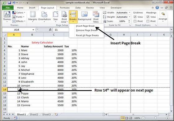
Insert vertical Page break − In this case, make sure to place the pointer in row 1. Choose Page Layout » Page Setup » Breaks » Insert Page Break to create the page break.
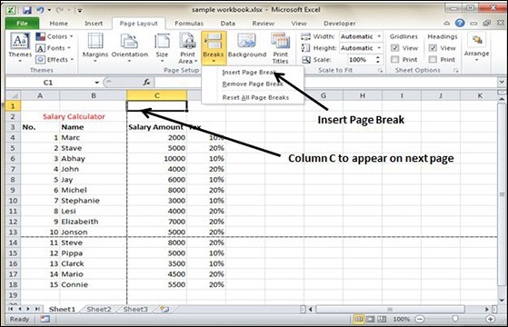
Removing Page Breaks
-
Remove a page break you’ve added − Move the cell pointer to the first row beneath the manual page break and then choose Page Layout » Page Setup » Breaks » Remove Page Break.
-
Remove all manual page breaks − Choose Page Layout » Page Setup » Breaks » Reset All Page Breaks.
Set Background in Excel 2010
Background Image
Unfortunately, you cannot have a background image on your printouts. You may have noticed the Page Layout » Page Setup » Background command. This button displays a dialogue box that lets you select an image to display as a background. Placing this control among the other print-related commands is very misleading. Background images placed on a worksheet are never printed.
Alternative to Placing Background
-
You can insert a Shape, WordArt, or a picture on your worksheet and then adjust its transparency. Then copy the image to all printed pages.
-
You can insert an object in a page header or footer.
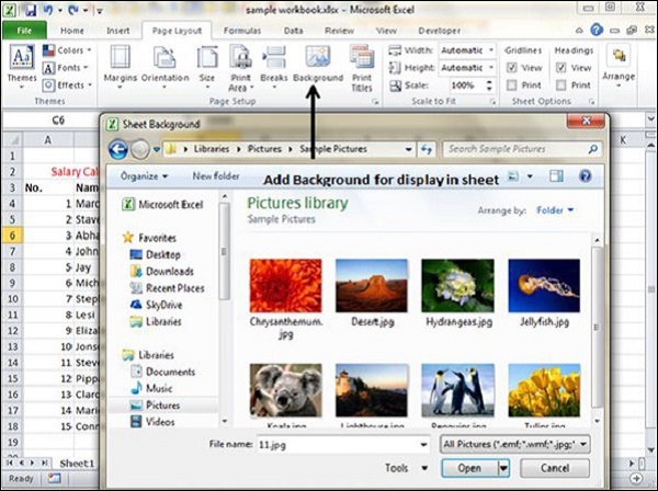
Freeze Panes in Excel 2010
Freezing Panes
If you set up a worksheet with row or column headings, these headings will not be visible when you scroll down or to the right. MS Excel provides a handy solution to this problem with freezing panes. Freezing panes keeps the headings visible while you’re scrolling through the worksheet.
Using Freeze Panes
Follow the steps mentioned below to freeze panes.
-
Select the First row or First Column or the row Below, which you want to freeze, or Column right to area, which you want to freeze.
-
Choose View Tab » Freeze Panes.
-
Select the suitable option −
-
Freeze Panes − To freeze area of cells.
-
Freeze Top Row − To freeze first row of worksheet.
-
Freeze First Column − To freeze first Column of worksheet.
-
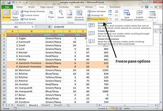
-
If you have selected Freeze top row you can see the first row appears at the top, after scrolling also. See the below screen-shot.
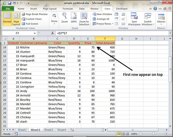
Unfreeze Panes
To unfreeze Panes, choose View Tab » Unfreeze Panes.
Conditional Format in Excel 2010
Conditional Formatting
MS Excel 2010 Conditional Formatting feature enables you to format a range of values so that the values outside certain limits, are automatically formatted.
Choose Home Tab » Style group » Conditional Formatting dropdown.
Various Conditional Formatting Options
-
Highlight Cells Rules − It opens a continuation menu with various options for defining the formatting rules that highlight the cells in the cell selection that contain certain values, text, or dates, or that have values greater or less than a particular value, or that fall within a certain ranges of values.
Suppose you want to find cell with Amount 0 and Mark them as red.Choose Range of cell » Home Tab » Conditional Formatting DropDown » Highlight Cell Rules » Equal To.
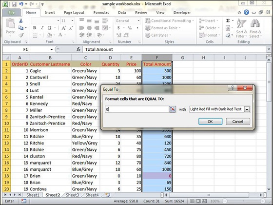
After Clicking ok, the cells with value zero are marked as red.
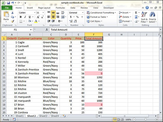
-
Top/Bottom Rules − It opens a continuation menu with various options for defining the formatting rules that highlight the top and bottom values, percentages, and above and below average values in the cell selection.
Suppose you want to highlight the top 10% rows you can do this with these Top/Bottom rules.
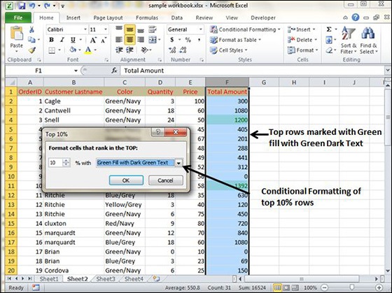
-
Data Bars − It opens a palette with different color data bars that you can apply to the cell selection to indicate their values relative to each other by clicking the data bar thumbnail.
With this conditional Formatting data Bars will appear in each cell.
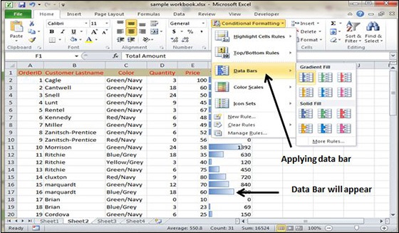
-
Color Scales − It opens a palette with different three- and two-colored scales that you can apply to the cell selection to indicate their values relative to each other by clicking the color scale thumbnail.
See the below screenshot with Color Scales, conditional formatting applied.
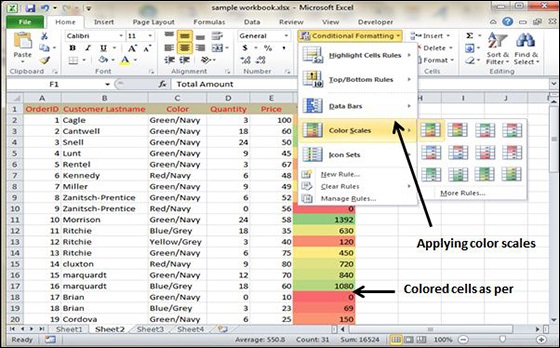
-
Icon Sets − It opens a palette with different sets of icons that you can apply to the cell selection to indicate their values relative to each other by clicking the icon set.
See the below screenshot with Icon Sets conditional formatting applied.
![]()
-
New Rule − It opens the New Formatting Rule dialog box, where you define a custom conditional formatting rule to apply to the cell selection.
-
Clear Rules − It opens a continuation menu, where you can remove the conditional formatting rules for the cell selection by clicking the Selected Cells option, for the entire worksheet by clicking the Entire Sheet option, or for just the current data table by clicking the This Table option.
-
Manage Rules − It opens the Conditional Formatting Rules Manager dialog box, where you edit and delete particular rules as well as adjust their rule precedence by moving them up or down in the Rules list box.
Creating Formulas in Excel 2010
Formulas in MS Excel
Formulas are the Bread and butter of worksheet. Without formula, worksheet will be just simple tabular representation of data. A formula consists of special code, which is entered into a cell. It performs some calculations and returns a result, which is displayed in the cell.
Formulas use a variety of operators and worksheet functions to work with values and text. The values and text used in formulas can be located in other cells, which makes changing data easy and gives worksheets their dynamic nature. For example, you can quickly change the data in a worksheet and formulas works.
Elements of Formulas
A formula can consist of any of these elements −
-
Mathematical operators, such as +(for addition) and *(for multiplication)
Example −
-
=A1+A2 Adds the values in cells A1 and A2.
-
-
Values or text
Example −
-
=200*0.5 Multiplies 200 times 0.15. This formula uses only values, and it always returns the same result as 100.
-
-
Cell references (including named cells and ranges)
Example −
-
=A1=C12 Compares cell A1 with cell C12. If the cells are identical, the formula returns TRUE; otherwise, it returns FALSE.
-
-
Worksheet functions (such as SUMor AVERAGE)
Example −
-
=SUM(A1:A12) Adds the values in the range A1:A12.
-
Creating Formula
For creating a formula you need to type in the Formula Bar. Formula begins with ‘=’ sign. When building formulas manually, you can either type in the cell addresses or you can point to them in the worksheet. Using the Pointing method to supply the cell addresses for formulas is often easier and more powerful method of formula building. When you are using built-in functions, you click the cell or drag through the cell range that you want to use when defining the function’s arguments in the Function Arguments dialog box. See the below screen shot.
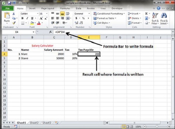
As soon as you complete a formula entry, Excel calculates the result, which is then displayed inside the cell within the worksheet (the contents of the formula, however, continue to be visible on the Formula bar anytime the cell is active). If you make an error in the formula that prevents Excel from being able to calculate the formula at all, Excel displays an Alert dialog box suggesting how to fix the problem.
Copying Formulas in Excel 2010
Copying Formulas in MS Excel
Copying formulas is one of the most common tasks that you do in a typical spreadsheet that relies primarily on formulas. When a formula uses cell references rather than constant values, Excel makes the task of copying an original formula to every place that requires a similar formula.
Relative Cell Addresses
MS Excel does it automatically adjusting the cell references in the original formula to suit the position of the copies that you make. It does this through a system known as relative cell addresses, where by the column references in the cell address in the formula change to suit their new column position and the row references change to suit their new row position.
Let us see this with the help of example. Suppose we want the sum of all the rows at last, then we will write a formula for first column i.e. B. We want sum of the rows from 3 to 8 in the 9th row.
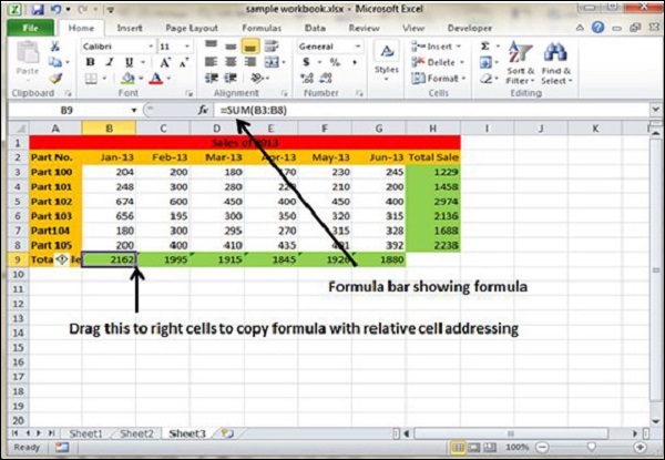
After writing formula in the 9th row, we can drag it to remaining columns and the formula gets copied. After dragging we can see the formula in the remaining columns as below.
-
column C : =SUM(C3:C8)
-
column D : =SUM(D3:D8)
-
column E : =SUM(E3:E8)
-
column F : =SUM(F3:F8)
-
column G : =SUM(G3:G8)
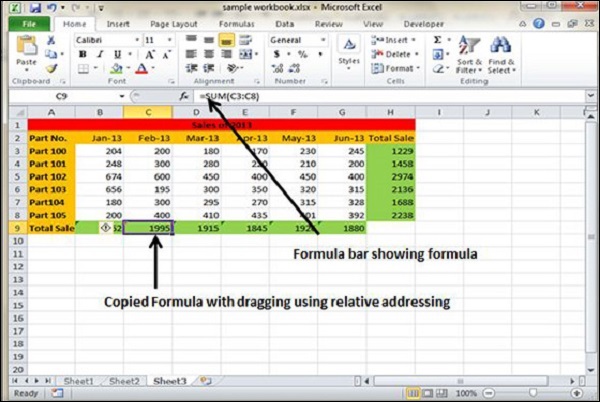
Formula Reference in Excel 2010
Cell References in Formulas
Most formulas you create include references to cells or ranges. These references enable your formulas to work dynamically with the data contained in those cells or ranges. For example, if your formula refers to cell C2 and you change the value contained in C2, the formula result reflects new value automatically. If you didn’t use references in your formulas, you would need to edit the formulas themselves in order to change the values used in the formulas.
When you use a cell (or range) reference in a formula, you can use three types of references − relative, absolute, and mixed references.
Relative Cell References
The row and column references can change when you copy the formula to another cell because the references are actually offsets from the current row and column. By default, Excel creates relative cell references in formulas.
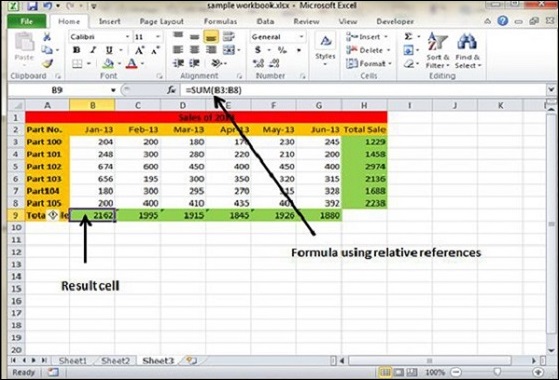
Absolute Cell References
The row and column references do not change when you copy the formula because the reference is to an actual cell address. An absolute reference uses two dollar signs in its address: one for the column letter and one for the row number (for example, $A$5).
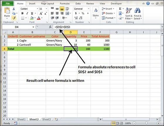
Mixed Cell References
Both the row or column reference is relative and the other is absolute. Only one of the address parts is absolute (for example, $A5 or A$5).
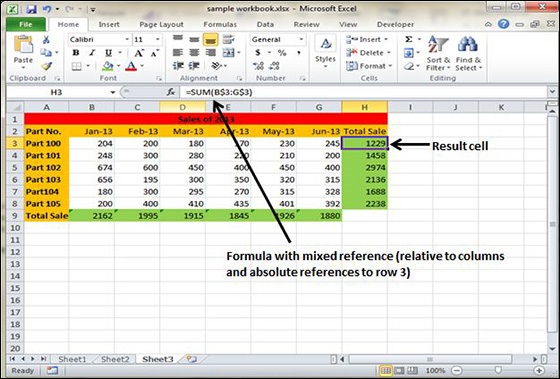
Using Functions in Excel 2010
Functions in Formula
Many formulas you create use available worksheet functions. These functions enable you to greatly enhance the power of your formulas and perform calculations that are difficult if you use only the operators. For example, you can use the LOG or SIN function to calculate the Logarithm or Sin ratio. You can’t do this complicated calculation by using the mathematical operators alone.
Using Functions
When you type = sign and then type any alphabet you will see the searched functions as below.
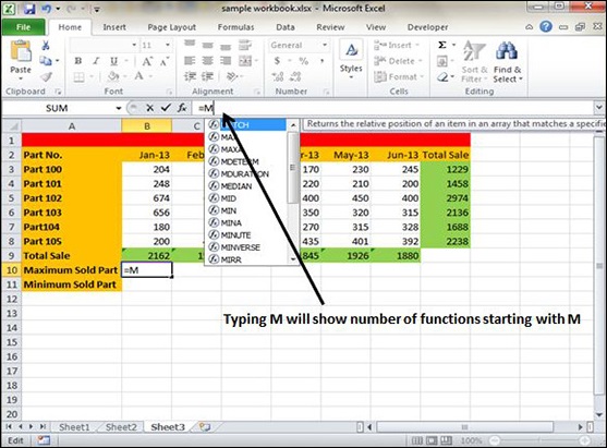
Suppose you need to determine the largest value in a range. A formula can’t tell you the answer without using a function. We will use formula that uses the MAX function to return the largest value in the range B3:B8 as =MAX(A1:D100).
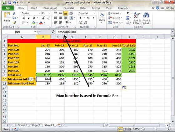
Another example of functions. Suppose you want to find if the cell of month is greater than 1900 then we can give Bonus to Sales representative. The we can achieve it with writing formula with IF functions as =IF(B9>1900,»Yes»,»No»)
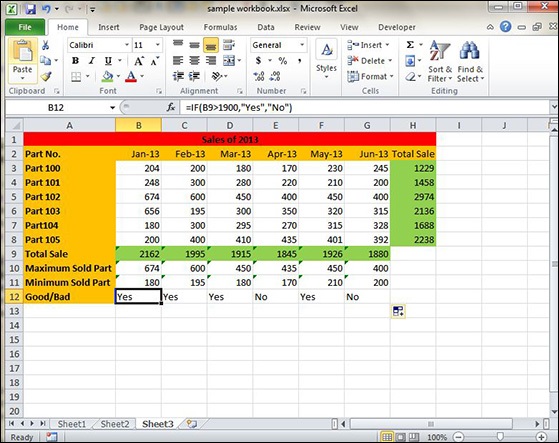
Function Arguments
In the above examples, you may have noticed that all the functions used parentheses. The information inside the parentheses is the list of arguments.
Functions vary in how they use arguments. Depending on what it has to do, a function may use.
-
No arguments − Examples − Now(), Date(), etc.
-
One argument − UPPER(), LOWER(), etc.
-
A fixed number of arguments − IF(), MAX(), MIN(), AVERGAGE(), etc.
-
Infinite number of arguments
-
Optional arguments
Built-in Functions in Excel 2010
Built In Functions
MS Excel has many built in functions, which we can use in our formula. To see all the functions by category, choose Formulas Tab » Insert Function. Then Insert function Dialog appears from which we can choose the function.
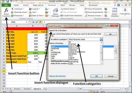
Functions by Categories
Let us see some of the built in functions in MS Excel.
-
Text Functions
-
LOWER − Converts all characters in a supplied text string to lower case
-
UPPER − Converts all characters in a supplied text string to upper case
-
TRIM − Removes duplicate spaces, and spaces at the start and end of a text string
-
CONCATENATE − Joins together two or more text strings.
-
LEFT − Returns a specified number of characters from the start of a supplied text string.
-
MID − Returns a specified number of characters from the middle of a supplied text string
-
RIGHT − Returns a specified number of characters from the end of a supplied text string.
-
LEN − Returns the length of a supplied text string
-
FIND − Returns the position of a supplied character or text string from within a supplied text string (case-sensitive).
-
-
Date & Time
-
DATE − Returns a date, from a user-supplied year, month and day.
-
TIME − Returns a time, from a user-supplied hour, minute and second.
-
DATEVALUE − Converts a text string showing a date, to an integer that represents the date in Excel’s date-time code.
-
TIMEVALUE − Converts a text string showing a time, to a decimal that represents the time in Excel.
-
NOW − Returns the current date & time.
-
TODAY − Returns today’s date.
-
-
Statistical
-
MAX − Returns the largest value from a list of supplied numbers.
-
MIN − Returns the smallest value from a list of supplied numbers.
-
AVERAGE − Returns the Average of a list of supplied numbers.
-
COUNT − Returns the number of numerical values in a supplied set of cells or values.
-
COUNTIF − Returns the number of cells (of a supplied range), that satisfies a given criteria.
-
SUM − Returns the sum of a supplied list of numbers
-
-
Logical
-
AND − Tests a number of user-defined conditions and returns TRUE if ALL of the conditions evaluate to TRUE, or FALSE otherwise
-
OR − Tests a number of user-defined conditions and returns TRUE if ANY of the conditions evaluate to TRUE, or FALSE otherwise.
-
NOT − Returns a logical value that is the opposite of a user supplied logical value or expression i.e. returns FALSE if the supplied argument is TRUE and returns TRUE if the supplied argument is FAL
-
-
Math & Trig
-
ABS − Returns the absolute value (i.e. the modulus) of a supplied number.
-
SIGN − Returns the sign (+1, -1 or 0) of a supplied number.
-
SQRT − Returns the positive square root of a given number.
-
MOD − Returns the remainder from a division between two supplied numbers.
-
Data Filtering in Excel 2010
Filters in MS Excel
Filtering data in MS Excel refers to displaying only the rows that meet certain conditions. (The other rows gets hidden.)
Using the store data, if you are interested in seeing data where Shoe Size is 36, then you can set filter to do this. Follow the below mentioned steps to do this.
-
Place a cursor on the Header Row.
-
Choose Data Tab » Filter to set filter.
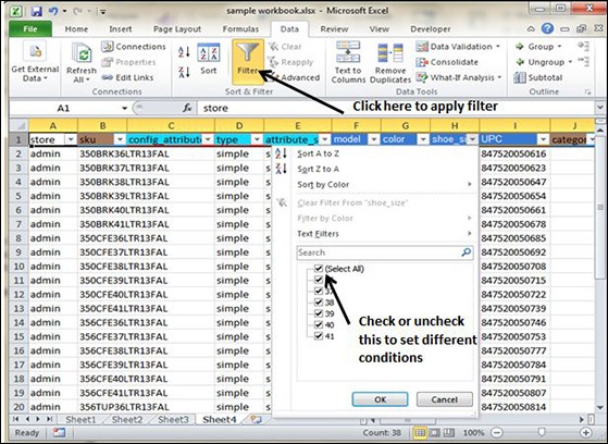
-
Click the drop-down arrow in the Area Row Header and remove the check mark from Select All, which unselects everything.
-
Then select the check mark for Size 36 which will filter the data and displays data of Shoe Size 36.
-
Some of the row numbers are missing; these rows contain the filtered (hidden) data.
-
There is drop-down arrow in the Area column now shows a different graphic — an icon that indicates the column is filtered.
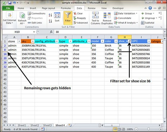
Using Multiple Filters
You can filter the records by multiple conditions i.e. by multiple column values. Suppose after size 36 is filtered, you need to have the filter where color is equal to Coffee. After setting filter for Shoe Size, choose Color column and then set filter for color.
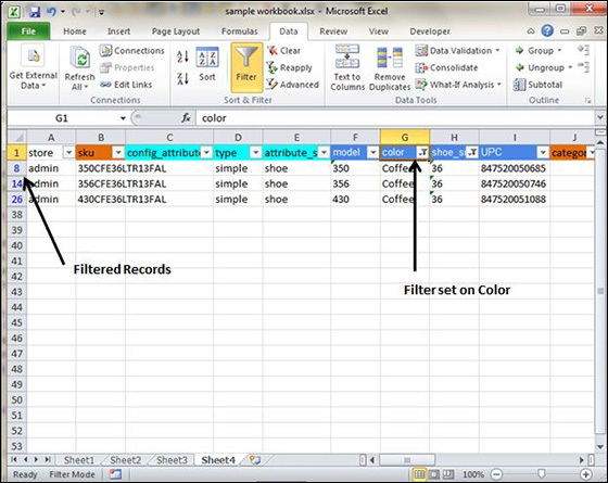
Data Sorting in Excel 2010
Sorting in MS Excel
Sorting data in MS Excel rearranges the rows based on the contents of a particular column. You may want to sort a table to put names in alphabetical order. Or, maybe you want to sort data by Amount from smallest to largest or largest to smallest.
To Sort the data follow the steps mentioned below.
- Select the Column by which you want to sort data.
- Choose Data Tab » Sort Below dialog appears.
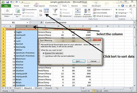
-
If you want to sort data based on a selected column, Choose Continue with the selection or if you want sorting based on other columns, choose Expand Selection.
-
You can Sort based on the below Conditions.
-
Values − Alphabetically or numerically.
-
Cell Color − Based on Color of Cell.
-
Font Color − Based on Font color.
-
Cell Icon − Based on Cell Icon.
-
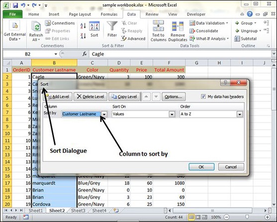
- Clicking Ok will sort the data.
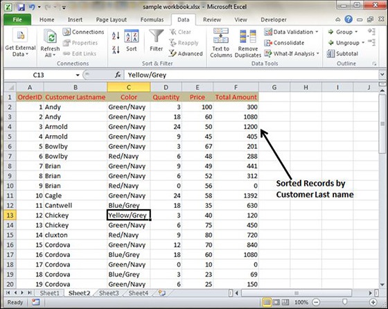
Sorting option is also available from the Home Tab. Choose Home Tab » Sort & Filter. You can see the same dialog to sort records.
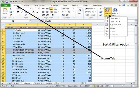
Using Ranges in Excel 2010
Ranges in MS Excel
A cell is a single element in a worksheet that can hold a value, some text, or a formula. A cell is identified by its address, which consists of its column letter and row number. For example, cell B1 is the cell in the second column and the first row.
A group of cells is called a range. You designate a range address by specifying its upper-left cell address and its lower-right cell address, separated by a colon.
Example of Ranges −
-
C24 − A range that consists of a single cell.
-
A1:B1 − Two cells that occupy one row and two columns.
-
A1:A100 − 100 cells in column A.
-
A1:D4 − 16 cells (four rows by four columns).
Selecting Ranges
You can select a range in several ways −
-
Press the left mouse button and drag, highlighting the range. Then release the mouse button. If you drag to the end of the screen, the worksheet will scroll.
-
Press the Shift key while you use the navigation keys to select a range.
-
Press F8 and then move the cell pointer with the navigation keys to highlight the range. Press F8 again to return the navigation keys to normal movement.
-
Type the cell or range address into the Name box and press Enter. Excel selects the cell or range that you specified.
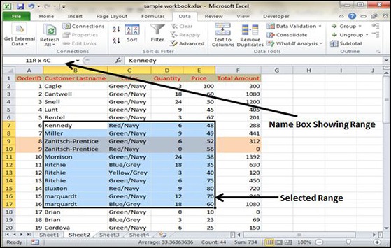
Selecting Complete Rows and Columns
When you need to select an entire row or column. You can select entire rows and columns in much the same manner as you select ranges −
-
Click the row or column border to select a single row or column.
-
To select multiple adjacent rows or columns, click a row or column border and drag to highlight additional rows or columns.
-
To select multiple (nonadjacent) rows or columns, press Ctrl while you click the row or column borders that you want.
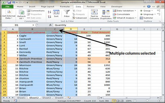
Data Validation in Excel 2010
Data Validation
MS Excel data validation feature allows you to set up certain rules that dictate what can be entered into a cell. For example, you may want to limit data entry in a particular cell to whole numbers between 0 and 10. If the user makes an invalid entry, you can display a custom message as shown below.
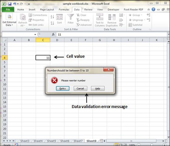
Validation Criteria
To specify the type of data allowable in a cell or range, follow the steps below, which shows all the three tabs of the Data Validation dialog box.
-
Select the cell or range.
-
Choose Data » Data Tools » Data Validation. Excel displays its Data Validation dialog box having 3 tabs settings, Input Message and Error alert.
Settings Tab
Here you can set the type of validation you need. Choose an option from the Allow drop-down list. The contents of the Data Validation dialog box will change, displaying controls based on your choice.
-
Any Value − Selecting this option removes any existing data validation.
-
Whole Number − The user must enter a whole number.For example, you can specify that the entry must be a whole number greater than or equal to 50.
-
Decimal − The user must enter a number. For example, you can specify that the entry must be greater than or equal to 10 and less than or equal to 20.
-
List − The user must choose from a list of entries you provide. You will create drop-down list with this validation. You have to give input ranges then those values will appear in the drop-down.
-
Date − The user must enter a date. You specify a valid date range from choices in the Data drop-down list. For example, you can specify that the entered data must be greater than or equal to January 1, 2013, and less than or equal to December 31, 2013.
-
Time − The user must enter a time. You specify a valid time range from choices in the Data drop-down list. For example, you can specify that the entered data must be later than 12:00 p.m.
-
Text Length − The length of the data (number of characters) is limited. You specify a valid length by using the Data drop-down list. For example, you can specify that the length of the entered data be 1 (a single alphanumeric character).
-
Custom − To use this option, you must supply a logical formula that determines the validity of the user’s entry (a logical formula returns either TRUE or FALSE).
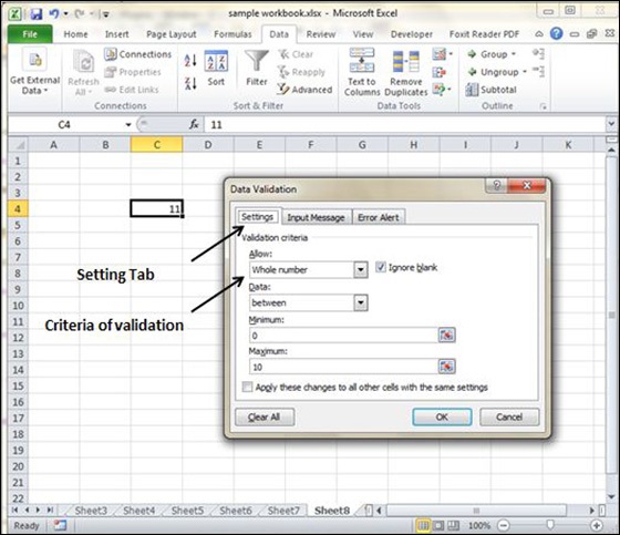
Input Message Tab
You can set the input help message with this tab. Fill the title and Input message of the Input message tab and the input message will appear when the cell is selected.
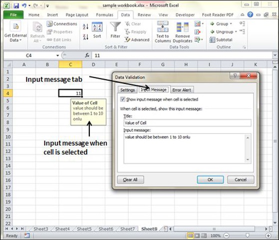
Error Alert Tab
You can specify an error message with this tab. Fill the title and error message. Select the style of the error as stop, warning or Information as per you need.
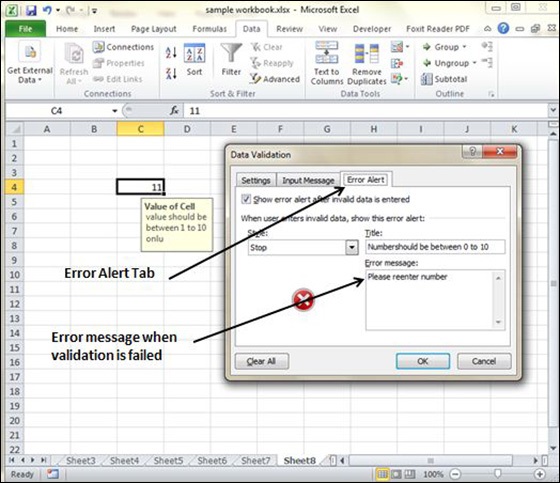
Using Styles in Excel 2010
Using Styles in MS Excel
With MS Excel 2010 Named styles make it very easy to apply a set of predefined formatting options to a cell or range. It saves time as well as make sure that look of the cells are consistent.
A Style can consist of settings for up to six different attributes −
- Number format
- Font (type, size, and color)
- Alignment (vertical and horizontal)
- Borders
- Pattern
- Protection (locked and hidden)
Now, let us see how styles are helpful. Suppose that you apply a particular style to some twenty cells scattered throughout your worksheet. Later, you realize that these cells should have a font size of 12 pt. rather than 14 pt. Rather than changing each cell, simply edit the style. All cells with that particular style change automatically.
Applying Styles
Choose Home » Styles » Cell Styles. Note that this display is a live preview, that is, as you move your mouse over the style choices, the selected cell or range temporarily displays the style. When you see a style you like, click it to apply the style to the selection.
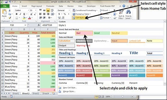
Creating Custom Style in MS Excel
We can create new custom style in Excel 2010. To create a new style, follow these steps −
- Select a cell and click on Cell styles from Home Tab.
- Click on New Cell Style and give style name.
- Click on Format to apply formatting to the cell.
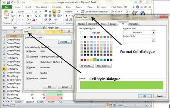
-
After applying formatting click on OK. This will add new style in the styles. You can view it on Home » Styles.
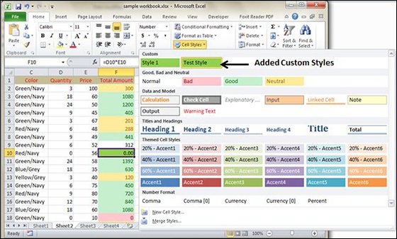
Using Themes in Excel 2010
Using Themes in MS Excel
To help users create more professional-looking documents, MS Excel has incorporated a concept known as document themes. By using themes, it is easy to specify the colors, fonts, and a variety of graphic effects in a document. And best of all, changing the entire look of your document is a breeze. A few mouse clicks is all it takes to apply a different theme and change the look of your workbook.
Applying Themes
Choose Page layout Tab » Themes Dropdown. Note that this display is a live preview, that is, as you move your mouse over the Theme, it temporarily displays the theme effect. When you see a style you like, click it to apply the style to the selection.
Creating Custom Theme in MS Excel
We can create new custom Theme in Excel 2010. To create a new style, follow these steps −
-
Click on the save current theme option under Theme in Page Layout Tab.
-
This will save the current theme to office folder.
-
You can browse the theme later to load the theme.
Using Templates in Excel 2010
Using Templates in MS Excel
Template is essentially a model that serves as the basis for something. An Excel template is a workbook that’s used to create other workbooks.
Viewing Available Templates
To view the Excel templates, choose File » New to display the available templates screen in Backstage View. You can select a template stored on your hard drive, or a template from Microsoft Office Online. If you choose a template from Microsoft Office Online, you must be connected to the Internet to download it. The Office Online Templates section contains a number of icons, which represents various categories of templates. Click an icon, and you’ll see the available templates. When you select a template thumbnail, you can see a preview in the right panel.
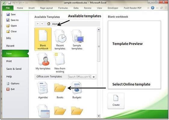
On-line Templates
These template data is available online at the Microsoft server. When you select the template and click on it, it will download the template data from Microsoft server and opens it as shown below.
Using Templates in MS Excel
Template is essentially a model that serves as the basis for something. An Excel template is a workbook that’s used to create other workbooks.
Viewing Available Templates
To view the Excel templates, choose File » New to display the available templates screen in Backstage View. You can select a template stored on your hard drive, or a template from Microsoft Office Online. If you choose a template from Microsoft Office Online, you must be connected to the Internet to download it. The Office Online Templates section contains a number of icons, which represents various categories of templates. Click an icon, and you’ll see the available templates. When you select a template thumbnail, you can see a preview in the right panel.
On-line Templates
These template data is available online at the Microsoft server. When you select the template and click on it, it will download the template data from Microsoft server and opens it as shown below.
Using Macros in Excel 2010
Macros in MS Excel
Macros enable you to automate almost any task that you can undertake in Excel 2010. By using macro recorder from View Tab » Macro Dropdown to record tasks that you perform routinely, you not only speed up the procedure considerably but you are assured that each step in a task is carried out the same way each and every time you perform a task.
To view macros choose View Tab » Macro dropdown.
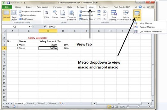
Macro Options
View tab contains a Macros command button to which a dropdown menu containing the following three options.
-
View Macros − Opens the Macro dialog box where you can select a macro to run or edit.
-
Record Macro − Opens the Record Macro dialog box where you define the settings for your new macro and then start the macro recorder; this is the same as clicking the Record Macro button on the Status bar.
-
Use Relative References − Uses relative cell addresses when recording a macro, making the macro more versatile by enabling you to run it in areas of a worksheet other than the ones originally used in the macro’s recording.
Creating Macros
You can create macros in one of two ways −
-
Use MS Excel’s macro recorder to record your actions as you undertake them in a worksheet.
-
Enter the instructions that you want to be followed in a VBA code in the Visual Basic Editor.
Now let’s create a simple macro that will automate the task of making cell content Bold and apply cell color.
- Choose View Tab » Macro dropdown.
- Click on Record Macro as below.
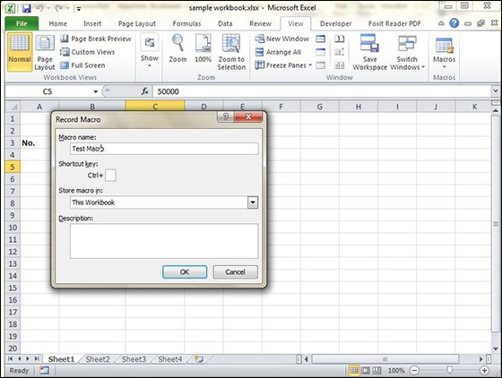
-
Now Macro recording will start.
-
Do the steps of action, which you want to perform repeatedly. Macro will record those steps.
-
You can stop the macro recording once done with all steps.
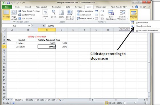
Edit Macro
You can edit the created Macro at any time. Editing macro will take you to the VBA programming editor.
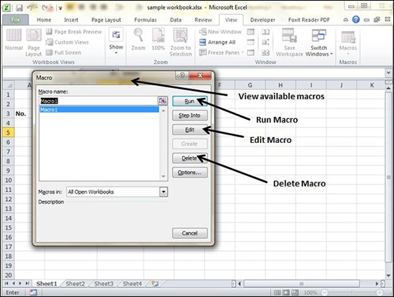
Adding Graphics in Excel 2010
Graphic Objects in MS Excel
MS Excel supports various types of graphic objects like Shapes gallery, SmartArt, Text Box, and WordArt available on the Insert tab of the Ribbon.Graphics are available in the Insert Tab. See the screenshots below for various available graphics in MS Excel 2010.
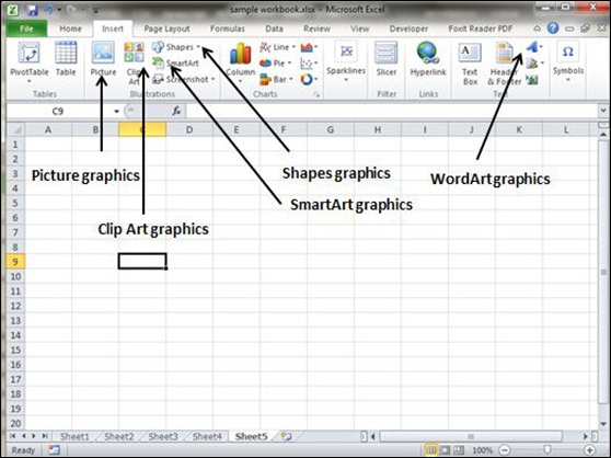
Insert Shape
-
Choose Insert Tab » Shapes dropdown.
-
Select the shape you want to insert. Click on shape to insert it.
-
To edit the inserted shape just drag the shape with the mouse. Shape will adjust the shape.
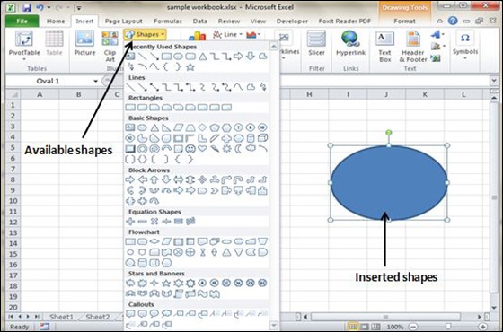
Insert Smart Art
-
Choose Insert Tab » SmartArt.
-
Clicking SmartArt will open the SmartArt dialogue as shown below in the screen-shot. Choose from the list of available smartArts.
-
Click on SmartArt to Insert it in the worksheet.
-
Edit the SmartArt as per your need.
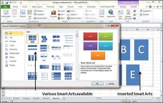
Insert Clip Art
-
Choose Insert Tab » Clip Art.
-
Clicking Clip Art will open the search box as shown in the below screen-shot. Choose from the list of available Clip Arts.
-
Click on Clip Art to Insert it in the worksheet.
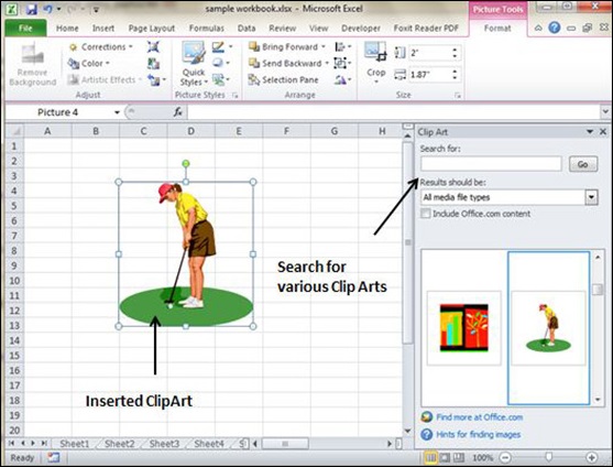
Insert Word Art
-
Choose Insert Tab » WordArt.
-
Select the style of WordArt, which you like and click it to enter a text in it.
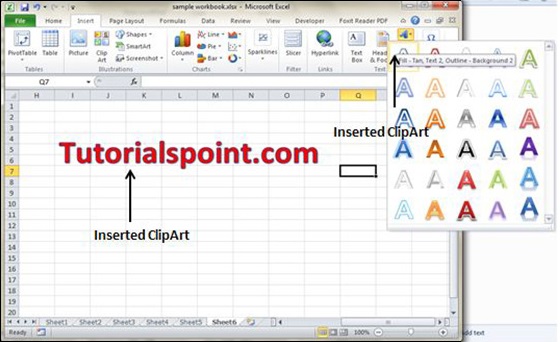
Cross Referencing in Excel 2010
Graphic Objects in MS Excel
When you have information spread across several different spreadsheets, it can seem a daunting task to bring all these different sets of data together into one meaningful list or table. This is where the Vlookup function comes into its own.
VLOOKUP
VlookUp searches for a value vertically down for the lookup table. VLOOKUP(lookup_value,table_array,col_index_num,range_lookup) has 4 parameters as below.
-
lookup_value − It is the user input. This is the value that the function uses to search on.
-
The table_array − It is the area of cells in which the table is located. This includes not only the column being searched on, but the data columns for which you are going to get the values that you need.
-
Col_index_num − It is the column of data that contains the answer that you want.
-
Range_lookup − It is a TRUE or FALSE value. When set to TRUE, the lookup function gives the closest match to the lookup_value without going over the lookup_value. When set to FALSE, an exact match must be found to the lookup_value or the function will return #N/A. Note, this requires that the column containing the lookup_value be formatted in ascending order.
VLOOKUP Example
Let’s look at a very simple example of cross-referencing two spreadsheets. Each spreadsheet contains information about the same group of people. The first spreadsheet has their dates of birth, and the second shows their favorite color. How do we build a list showing the person’s name, their date of birth and their favorite color? VLOOOKUP will help in this case. First of all, let us see data in both the sheets.
This is data in the first sheet
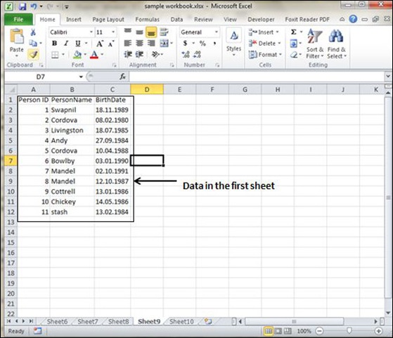
This is data in the second sheet
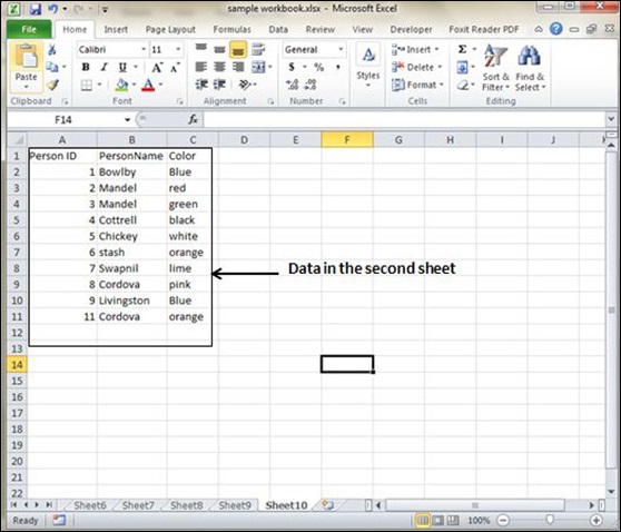
Now for finding the respective favorite color for that person from another sheet we need to vlookup the data. First argument to the VLOOKUP is lookup value (In this case it is person name). Second argument is the table array, which is table in the second sheet from B2 to C11. Third argument to VLOOKUP is Column index num, which is the answer we are looking for. In this case, it is 2 the color column number is 2. The fourth argument is True returning partial match or false returning exact match. After applying VLOOKUP formula it will calculate the color and the results are displayed as below.
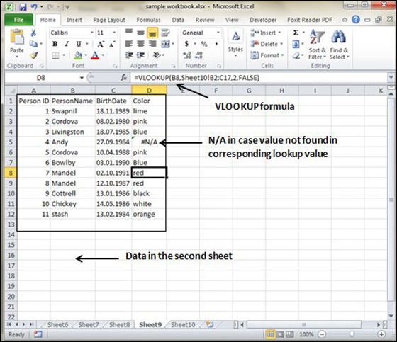
As you can see in the above screen-shot that results of VLOOKUP has searched for color in the second sheet table. It has returned #N/A in case where match is not found. In this case, Andy’s data is not present in the second sheet so it returned #N/A.
Printing Worksheets in Excel 2010
Quick Print
If you want to print a copy of a worksheet with no layout adjustment, use the Quick Print option. There are two ways in which we can use this option.
-
Choose File » Print (which displays the Print pane), and then click the Print button.
-
Press Ctrl+P and then click the Print button (or press Enter).
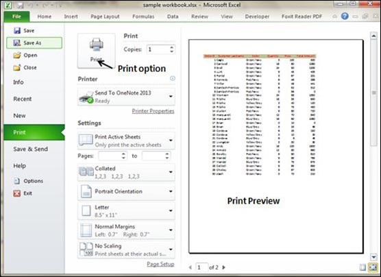
Adjusting Common Page Setup Settings
You can adjust the print settings available in the Page setup dialogue in different ways as discussed below. Page setup options include Page orientation, Page Size, Page Margins, etc.
-
The Print screen in Backstage View, displayed when you choose File » Print.
-
The Page Layout tab of the Ribbon.
Choosing Your Printer
To switch to a different printer, choose File » Print and use the drop-down control in the Printer section to select any other installed printer.
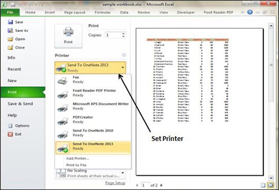
Specifying What You Want to Print
Sometimes you may want to print only a part of the worksheet rather than the entire active area. Choose File » Print and use the controls in the Settings section to specify what to print.
-
Active Sheets − Prints the active sheet or sheets that you selected.
-
Entire Workbook − Prints the entire workbook, including chart sheets.
-
Selection − Prints only the range that you selected before choosing File » Print.
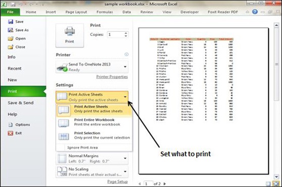
Email Workbooks MS Excel 2010
Email Workbook
MS Excel allows you to email the workbook very easily. To email the workbook to anyone, follow the below mentioned steps.
-
Choose File » Save and Send. It basically saves the document first and then the emails.
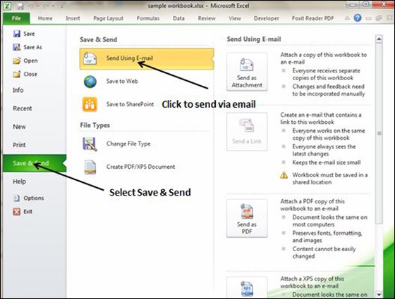
-
Click on Send using E-mail if your email system is configured. MS Outlook will open with the file as attachment in the New Email Window. You can send mail this workbook to anyone with valid email address.
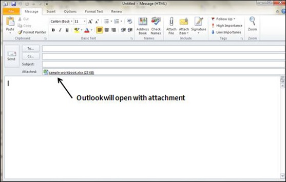
Translate Worksheet in Excel 2010
Translate Worksheet
You can translate the text written in a different language, such as phrases or paragraphs, individual words (by using the Mini Translator), or translate your whole file with MS Excel 2010.
Translation is available in the review tab of the ribbon in MS Excel 2010. You can quickly translate cell into different language with this option.
Performing Translation Step By Step
-
Select the content, which you want to translate to a different language.
-
Choose review tab » translation.
-
It will open the pane from which you can select the language to which you need to translate.
-
You need to have an internet connection for performing translation. It will translate using the Microsoft Translator.
-
Click on Insert to apply translation changes.
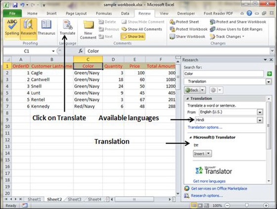
Workbook Security in Excel 2010
Workbook Security
We can apply security to the workbook by the concept of protection available in the Review Tab of ribbon. MS Excel’s protection-related features fall into three categories.
-
Worksheet protection − Protecting a worksheet from being modified, or restricting the modifications to certain users.
-
Workbook protection − Protecting a workbook from having sheets inserted or deleted, and also requiring the use of password to open the workbook.
Protect Worksheet
You may want to protect a worksheet for a variety of reasons. One reason is to prevent yourself or others from accidentally deleting the formulas or other critical data. A common scenario is to protect a worksheet, so that the data can be changed, but the formulas can’t be changed.
To protect a worksheet, choose Review » Changes group » Protect Sheet. Excel displays the Protect Sheet dialog box. Note that providing a password is optional. If you enter a password, that password will be required to unprotect the worksheet. You can select various options in which the sheet should be protected. Suppose we checked Format Cells option then Excel will not allow to format cells.
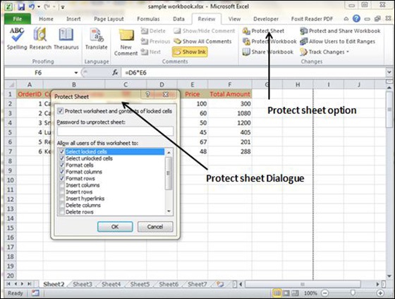
When somebody tries to format the cells, he or she will get the error as shown in the screenshot below.
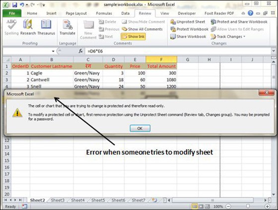
To unprotect a protected sheet, choose Review » Changes group » Unprotect Sheet. If the sheet was protected with a password, you’re prompted to enter that password.
Protecting a Workbook
Excel provides three ways to protect a workbook.
-
Requires a password to open the workbook.
-
Prevents the users from adding sheets, deleting sheets, hiding sheets, and unhiding sheets.
-
Prevents users from changing the size or position of windows.
Requiring a Password to Open a Workbook
Excel lets you save a workbook with a password. After doing so, whoever tries to open the workbook, must enter the password. To add a password to a workbook, follow these steps.
-
Choose File » Info » Protect Workbook » Encrypt With Password. Excel displays the Encrypt Document dialog box.
-
Type a password and click OK.
-
Type the password again and click OK.
-
Save the workbook.
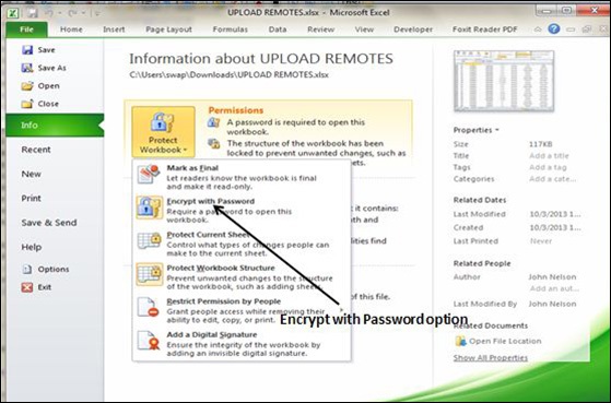
To remove a password from a workbook, repeat the same procedure. In Step 2, however, delete the existing password symbols.
Protecting Workbook’s Structure and Windows
To prevent others (or yourself) from performing certain actions in a workbook, you can protect the workbook’s structure and windows. When a workbook’s structure and windows are protected, the user may not Add a sheet, Delete a sheet, Hide a sheet, unhide a sheet, etc., and may not be allowed to change the size or position of a workbook’s windows respectively.
To protect a worksheet’s structure and windows, follow the below mentioned steps.
-
Choose Review » Changes group » Protect Workbook to display the Protect Workbook dialog box.
-
In the Protect Workbook dialog box, select the Structure check box and Windows check box.
-
(Optional) Enter a password.
-
Click OK.
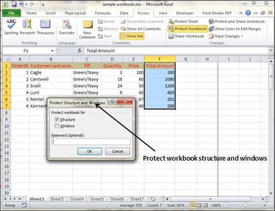
Data Tables in Excel 2010
Data Tables
In Excel, a Data Table is a way to see different results by altering an input cell in your formula. Data tables are available in Data Tab » What-If analysis dropdown » Data table in MS Excel.
Data Table with Example
Now, let us see data table concept with an example. Suppose you have the Price and quantity of many values. Also, you have the discount for that as third variable for calculating the Net Price. You can keep the Net Price value in the organized table format with the help of the data table. Your Price runs horizontally to the right while quantity runs vertically down. We are using a formula to calculate the Net Price as Price multiplied by Quantity minus total discount (Quantity * Discount for each quantity).
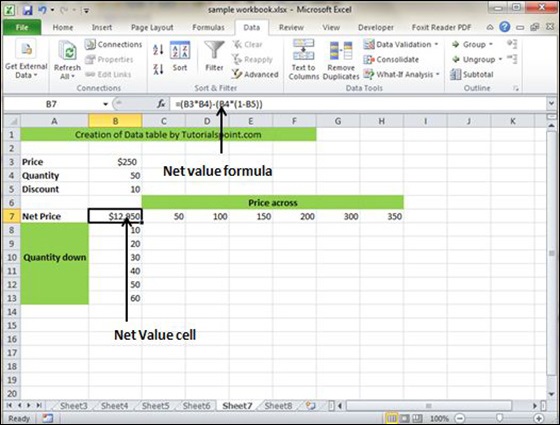
Now, for creation of data table select the range of data table. Choose Data Tab » What-If analysis dropdown » Data table. It will give you dialogue asking for Input row and Input Column. Give the Input row as Price cell (In this case cell B3) and Input column as quantity cell (In this case cell B4). Please see the below screen-shot.
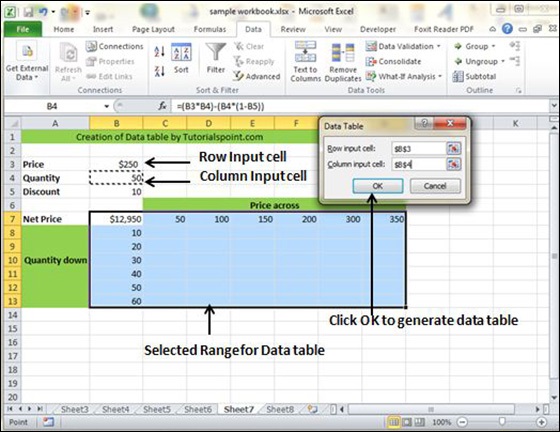
Clicking OK will generate data table as shown in the below screen-shot. It will generate the table formula. You can change the price horizontally or quantity vertically to see the change in the Net Price.
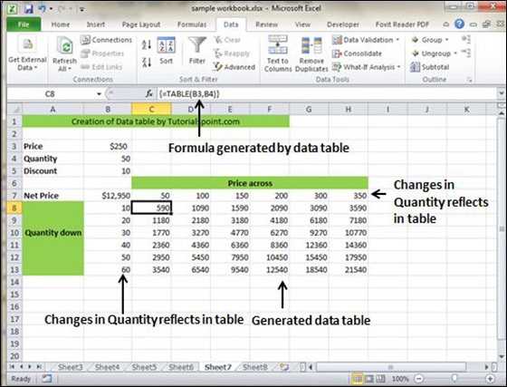
Pivot Tables in Excel 2010
Pivot Tables
A pivot table is essentially a dynamic summary report generated from a database. The database can reside in a worksheet (in the form of a table) or in an external data file. A pivot table can help transform endless rows and columns of numbers into a meaningful presentation of the data. Pivot tables are very powerful tool for summarized analysis of the data.
Pivot tables are available under Insert tab » PivotTable dropdown » PivotTable.
Pivot Table Example
Now, let us see Pivot table with the help of example. Suppose you have huge data of voters and you want to see the summarized data of voter Information per party, then you can use the Pivot table for it. Choose Insert tab » Pivot Table to insert pivot table. MS Excel selects the data of the table. You can select the pivot table location as existing sheet or new sheet.
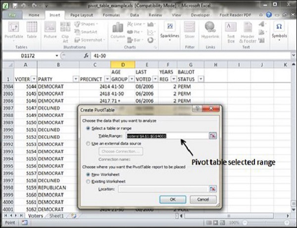
This will generate the Pivot table pane as shown below. You have various options available in the Pivot table pane. You can select fields for the generated pivot table.
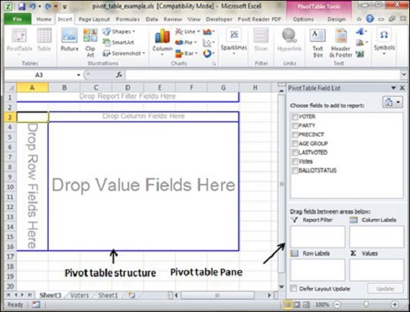
-
Column labels − A field that has a column orientation in the pivot table. Each item in the field occupies a column.
-
Report Filter − You can set the filter for the report as year, then data gets filtered as per the year.
-
Row labels − A field that has a row orientation in the pivot table. Each item in the field occupies a row.
-
Values area − The cells in a pivot table that contain the summary data. Excel offers several ways to summarize the data (sum, average, count, and so on).
After giving input fields to the pivot table, it generates the pivot table with the data as shown below.
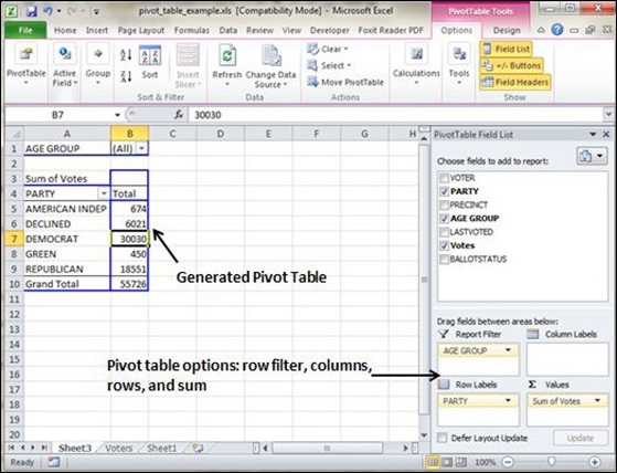
Simple Charts in Excel 2010
Charts
A chart is a visual representation of numeric values. Charts (also known as graphs) have been an integral part of spreadsheets. Charts generated by early spreadsheet products were quite crude, but thy have improved significantly over the years. Excel provides you with the tools to create a wide variety of highly customizable charts. Displaying data in a well-conceived chart can make your numbers more understandable. Because a chart presents a picture, charts are particularly useful for summarizing a series of numbers and their interrelationships.
Types of Charts
There are various chart types available in MS Excel as shown in the below screen-shot.
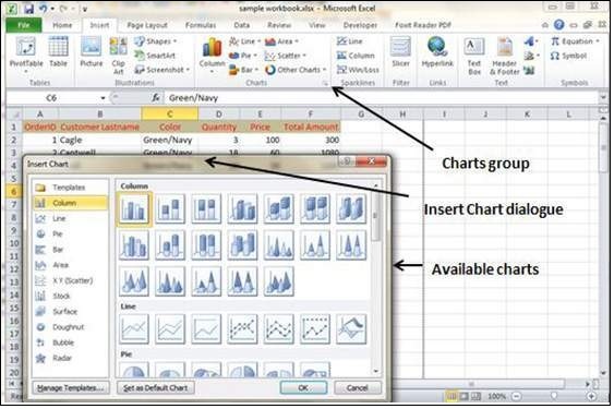
-
Column − Column chart shows data changes over a period of time or illustrates comparisons among items.
-
Bar − A bar chart illustrates comparisons among individual items.
-
Pie − A pie chart shows the size of items that make up a data series, proportional to the sum of the items. It always shows only one data series and is useful when you want to emphasize a significant element in the data.
-
Line − A line chart shows trends in data at equal intervals.
-
Area − An area chart emphasizes the magnitude of change over time.
-
X Y Scatter − An xy (scatter) chart shows the relationships among the numeric values in several data series, or plots two groups of numbers as one series of xy coordinates.
-
Stock − This chart type is most often used for stock price data, but can also be used for scientific data (for example, to indicate temperature changes).
-
Surface − A surface chart is useful when you want to find the optimum combinations between two sets of data. As in a topographic map, colors and patterns indicate areas that are in the same range of values.
-
Doughnut − Like a pie chart, a doughnut chart shows the relationship of parts to a whole; however, it can contain more than one data series.
-
Bubble − Data that is arranged in columns on a worksheet, so that x values are listed in the first column and corresponding y values and bubble size values are listed in adjacent columns, can be plotted in a bubble chart.
-
Radar − A radar chart compares the aggregate values of a number of data series.
Creating Chart
To create charts for the data by below mentioned steps.
-
Select the data for which you want to create the chart.
-
Choose Insert Tab » Select the chart or click on the Chart group to see various chart types.
-
Select the chart of your choice and click OK to generate the chart.
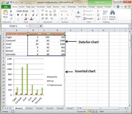
Editing Chart
You can edit the chart at any time after you have created it.
-
You can select the different data for chart input with Right click on chart » Select data. Selecting new data will generate the chart as per the new data, as shown in the below screen-shot.
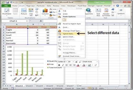
-
You can change the X axis of the chart by giving different inputs to X-axis of chart.
-
You can change the Y axis of chart by giving different inputs to Y-axis of chart.
Pivot Charts Excel 2010
Pivot Charts
A pivot chart is a graphical representation of a data summary, displayed in a pivot table. A pivot chart is always based on a pivot table. Although Excel lets you create a pivot table and a pivot chart at the same time, you can’t create a pivot chart without a pivot table. All Excel charting features are available in a pivot chart.
Pivot charts are available under Insert tab » PivotTable dropdown » PivotChart.
Pivot Chart Example
Now, let us see Pivot table with the help of an example. Suppose you have huge data of voters and you want to see the summarized view of the data of voter Information per party in the form of charts, then you can use the Pivot chart for it. Choose Insert tab » Pivot Chart to insert the pivot table.
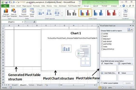
MS Excel selects the data of the table. You can select the pivot chart location as an existing sheet or a new sheet. Pivot chart depends on automatically created pivot table by the MS Excel. You can generate the pivot chart in the below screen-shot.
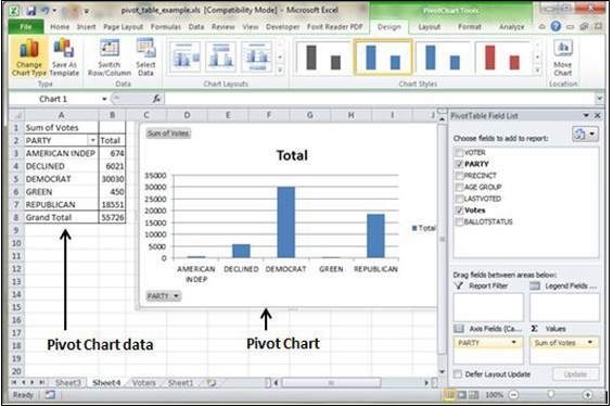
Keyboard Shortcuts in Excel 2010
MS Excel Keyboard Short-cuts
MS Excel offers many keyboard short-cuts. If you are familiar with windows operating system, you should be aware of most of them. Below is the list of all the major shortcut keys in Microsoft Excel.
-
Ctrl + A − Selects all contents of the worksheet.
-
Ctrl + B − Bold highlighted selection.
-
Ctrl + I − Italicizes the highlighted selection.
-
Ctrl + K − Inserts link.
-
Ctrl + U − Underlines the highlighted selection.
-
Ctrl + 1 − Changes the format of selected cells.
-
Ctrl + 5 − Strikethrough the highlighted selection.
-
Ctrl + P − Brings up the print dialog box to begin printing.
-
Ctrl + Z − Undo last action.
-
Ctrl + F3 − Opens Excel Name Manager.
-
Ctrl + F9 − Minimizes the current window.
-
Ctrl + F10 − Maximize currently selected window.
-
Ctrl + F6 − Switches between open workbooks or windows.
-
Ctrl + Page up − Moves between Excel work sheets in the same Excel document.
-
Ctrl + Page down − Moves between Excel work sheets in the same Excel document.
-
Ctrl + Tab − Moves between Two or more open Excel files.
-
Alt + = − Creates a formula to sum all of the above cells
-
Ctrl + ‘ − Inserts the value of the above cell into cell currently selected.
-
Ctrl + Shift + ! − Formats the number in comma format.
-
Ctrl + Shift + $ − Formats the number in currency format.
-
Ctrl + Shift + # − Formats the number in date format.
-
Ctrl + Shift + % − Formats the number in percentage format.
-
Ctrl + Shift + ^ − Formats the number in scientific format.
-
Ctrl + Shift + @ − Formats the number in time format.
-
Ctrl + Arrow key − Moves to the next section of text.
-
Ctrl + Space − Selects the entire column.
-
Shift + Space − Selects the entire row.
-
Ctrl + — − Deletes the selected column or row.
-
Ctrl + Shift + = − Inserts a new column or row.
-
Ctrl + Home − Moves to cell A1.
-
Ctrl + ~ − Switches between showing Excel formulas or their values in cells.
-
F2 − Edits the selected cell.
-
F3 − After a name has been created F3 will paste names.
-
F4 − Repeat last action. For example, if you changed the color of text in another cell pressing F4 will change the text in cell to the same color.
-
F5 − Goes to a specific cell. For example, C6.
-
F7 − Spell checks the selected text or document.
-
F11 − Creates chart from the selected data.
-
Ctrl + Shift + ; − Enters the current time.
-
Ctrl + ; − Enters the current date.
-
Alt + Shift + F1 − Inserts New Worksheet.
-
Alt + Enter − While typing text in a cell pressing Alt + Enter will move to the next line allowing for multiple lines of text in one cell.
-
Shift + F3 − Opens the Excel formula window.
-
Shift + F5 − Brings up the search box.