What can you do with excel 2013 - Word и Excel - помощь в работе с программами

Note: SkyDrive is now OneDrive, and SkyDrive Pro is now OneDrive for Business. Read more about this change at From SkyDrive to OneDrive.

The first thing you’ll see when you open Excel is a brand new look. It’s cleaner, but it’s also designed to help you get professional-looking results quickly. You’ll find many new features that let you get away from walls of numbers and draw more persuasive pictures of your data, guiding you to better, more informed decisions.

Tip: To learn how you can get started creating a basic Excel workbook quickly, see Basic tasks in Excel.

Top features to explore

Get started quickly

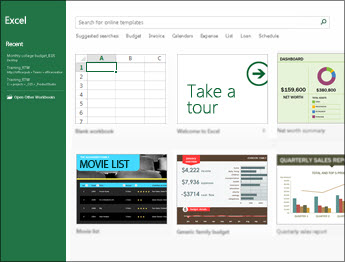
Templates do most of the set-up and design work for you, so you can focus on your data. When you open Excel 2013, you’ll see templates for budgets, calendars, forms, and reports, and more.

Instant data analysis

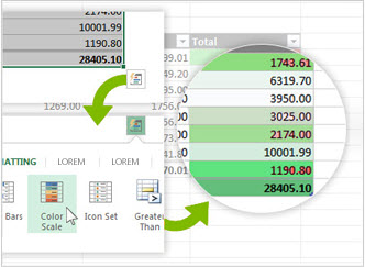
The new Quick Analysis tool lets you convert your data into a chart or table in two steps or less. Preview your data with conditional formatting, sparklines, or charts, and make your choice stick in just one click. To use this new feature, see Analyze your data instantly.

Fill out an entire column of data in a flash

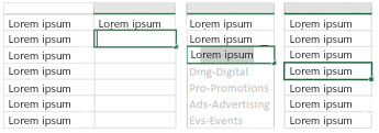
Flash Fill is like a data assistant that finishes your work for you. As soon as it detects what you want to do, Flash Fill enters the rest of your data in one fell swoop, following the pattern it recognizes in your data. To see when this feature comes in handy, see Split a column of data based on what you type.

Create the right chart for your data

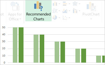
With Chart recommendations, Excel recommends the most suitable charts for your data. Get a quick peek to see how your data looks in the different charts, and then simply pick the one that shows the insights you want to present. Give this feature a try when you create a chart from start to finish.

Filter table data by using slicers

First introduced in Excel 2010 as an interactive way to filter PivotTable data, slicers can now also filter data in Excel tables, query tables, and other data tables. Simpler to set up and use, slicers show the current filter so you’ll know exactly what data you’re looking at.

One workbook, one window

In Excel 2013 each workbook has in its own window, making it easier to work on two workbooks at once. It also makes life easier when you’re working on two monitors.

New Excel functions

You’ll find several new functions in the math and trigonometry, statistical, engineering, date and time, lookup and reference, logical, and text function categories. Also new are a few Web service functions for referencing existing Representational State Transfer (REST)-compliant Web services. Look for details in New functions in Excel 2013.

Save and share files online

Excel makes it easier to save your workbooks to your own online location, like your free OneDrive or your organization’s Microsoft 365 service. It’s also simpler to share your worksheets with other people. No matter what device they’re using or where they are, everyone works with the latest version of a worksheet— and you can even work together in real time.

Embed worksheet data in a web page

To share part of your worksheet on the web, you can simply embed it on your web page. Other people can then work with the data in Excel for the web or open the embedded data in Excel.

Share an Excel worksheet in an online meeting

No matter where you are or what device you’re on—be it your smartphone, tablet, or PC—as long as you have Lync installed, you can connect to and share a workbook in an online meeting.

Save to a new file format

Now you can save to and open files in the new Strict Open XML Spreadsheet (*.xlsx) file format. This file format lets you read and write ISO8601 dates to resolve a leap year issue for the year 1900. To learn more about it, see Save a workbook in another file format.

New charting features

Changes to the ribbon for charts

The new Recommended Charts button on the Insert tab lets you pick from a variety of charts that are right for your data. Related types of charts like scatter and bubble charts are under one umbrella. And there’s a brand new button for combo charts—a favorite chart you’ve asked for. When you click a chart, you’ll also see a simpler Chart Tools ribbon. With just a Design and Format tab, it should be easier to find what you need.

Fine tune charts quickly

Three new chart buttons let you quickly pick and preview changes to chart elements (like titles or labels), the look and style of your chart, or to the data that is shown. To learn more about it, see Format elements of a chart.

Richer data labels

Now you can include rich and refreshable text from data points or any other text in your data labels, enhance them with formatting and additional freeform text, and display them in just about any shape. Data labels stay in place, even when you switch to a different type of chart. You can also connect them to their data points with leader lines on all charts, not just pie charts. To work with rich data labels, see Change the format of data labels in a chart.

View animation in charts

See a chart come alive when you make changes to its source data. This isn’t just fun to watch—the movement in the chart also makes the changes in your data much clearer.

Powerful data analysis

Create a PivotTable that suits your data

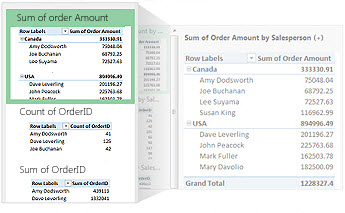
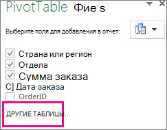
Picking the right fields to summarize your data in a PivotTable report can be a daunting task. Now you can get some help with that. When you create a PivotTable, Excel recommends several ways to summarize your data, and shows you a quick preview of the field layouts so you can pick the one that gives you the insights you’re looking for. To learn more about it, see Create a PivotTable to analyze worksheet data.

Use one Field List to create different types of PivotTables

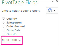
Create the layout of a PivotTable that uses one table or multiple tables by using one and the same Field List. Revamped to accommodate both single and multi-table PivotTables, the Field List makes it easier to find the fields you want in your PivotTable layout, switch to the new Excel Data Model by adding more tables, and explore and navigate to all of the tables. To learn more about it, see Use the Field List to arrange fields in a PivotTable.

Use multiple tables in your data analysis

The new Excel Data Model lets you to tap into powerful analysis features that were previously only available by installing the Power Pivot add-in. In addition to creating traditional PivotTables, you can now create PivotTables based on multiple tables in Excel. By importing different tables, and creating relationships between them, you’ll be able to analyze your data with results you aren’t able to get from traditional PivotTable data. To learn more about it, see Create a Data Model in Excel.

Power Query

If you’re using Office Professional Plus 2013 or Microsoft 365 Apps for enterprise, you can take advantage of Power Query for Excel. Use Power Query to easily discover and connect to data from public and corporate data sources. This includes new data search capabilities, as well as capabilities to easily transform and merge data from multiple data sources so that you can continue to analyze it in Excel. To learn more about it, see Discover and combine with Power Query for Excel.

Power Map

If you’re using Microsoft 365 Apps for enterprise, Office 2013, or Excel 2013, you can take advantage of Power Map for Excel. Power Map is a three-dimensional (3-D) data visualization tool that lets you look at information in new ways by using geographic and time-based data. You can discover insights that you might not see in traditional two-dimensional (2-D) tables and charts. Power Map is built into Microsoft 365 Apps for enterprise, but you’ll need to download a preview version to use it with Office 2013 or Excel 2013. See Power Map for Excel for details about the preview. To learn more about using Power Map to create a visual 3-D tour of your data, see Get started with Power Map.

Connect to new data sources

To use multiple tables in the Excel Data Model, you can now connect to and import data from additional data sources into Excel as tables or PivotTables. For example, connect to data feeds like OData, Windows Azure DataMarket, and SharePoint data feeds. You can also connect to data sources from additional OLE DB providers.

Create relationships between tables

When you’ve got data from different data sources in multiple tables in the Excel Data Model, creating relationships between those tables makes it easy to analyze your data without having to consolidate it into one table. By using MDX queries, you can further leverage table relationships to create meaningful PivotTable reports. To learn more about it, see Create a relationship between two tables.

Use a timeline to show data for different time periods

A timeline makes it simpler to compare your PivotTable or PivotChart data over different time periods. Instead of grouping by dates, you can now simply filter dates interactively or move through data in sequential time periods, like rolling month-to-month performance, in just one click. To learn more about it, see Create a PivotTable timeline to filter dates.

Use Drill Down, Drill Up, and Cross Drill to get to different levels of detail

Drilling down to different levels of detail in a complex set of data is not an easy task. Custom sets are helpful, but finding them among a large number of fields in the Field List takes time. In the new Excel Data Model, you’ll be able to navigate to different levels more easily. Use Drill Down into a PivotTable or PivotChart hierarchy to see granular levels of detail, and Drill Up to go to a higher level for “big picture” insights. To learn more about it, see Drill into PivotTable data.

Use OLAP calculated members and measures

Tap into the power of self-service Business Intelligence (BI) and add your own Multidimensional Expression (MDX)-based calculations in PivotTable data that is connected to an Online Analytical Processing (OLAP) cube. No need to reach for the Excel Object Model—now you can create and manage calculated members and measures right in Excel.

Create a standalone PivotChart

A PivotChart no longer has to be associated with a PivotTable. A standalone or de-coupled PivotChart lets you experience new ways to navigate to data details by using the new Drill Down, and Drill Up features. It’s also much easier to copy or move a de-coupled PivotChart. To learn more about it, see Create a PivotChart.

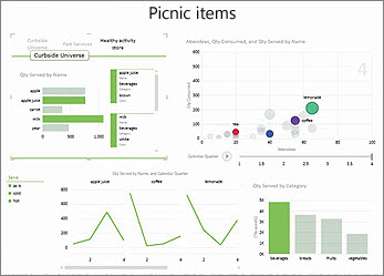
Power View

If you’re using Office Professional Plus, you can take advantage of Power View. Simply click the Power View button on the ribbon to discover insights about your data with highly interactive, powerful data exploration, visualization, and presentation features that are easy to apply. Power View lets you create and interact with charts, slicers, and other data visualizations in a single sheet.

New and improved add-ins and converters

Power Pivot for Excel add-in

If you’re using Office Professional Plus 2013 or Microsoft 365 Apps for enterprise, the Power Pivot add-in comes installed with Excel. The Power Pivot data analysis engine is now built into Excel so that you can build simple data models directly in Excel. The Power Pivot add-in provides an environment for creating more sophisticated models. Use it to filter out data when importing it, define your own hierarchies, calculation fields, and key performance indicators (KPIs), and use the Data Analysis Expressions (DAX) language to create advanced formulas.

Inquire add-in

If you’re using Office Professional Plus 2013 or Microsoft 365 Apps for enterprise, the Inquire add-in comes installed with Excel. It helps you analyze and review your workbooks to understand their design, function, and data dependencies, and to uncover a variety of problems including formula errors or inconsistencies, hidden information, broken links and others. From Inquire, you can start a new Microsoft Office tool, called Spreadsheet Compare, to compare two versions of a workbook, clearly indicating where changes have occurred. During an audit, you have full visibility of the changes in your workbooks.

Источник

Примечание: Служба SkyDrive теперь называется OneDrive, а приложение SkyDrive Pro — OneDrive для бизнеса. Дополнительные сведения об этих изменениях можно найти в статье От SkyDrive к OneDrive.

В первую очередь выделяется новый внешний вид Excel. Он избавлен от лишних деталей, но также рассчитан на быстрое достижение профессиональных результатов. Добавлено множество функций, помогающих ориентироваться в большом количестве чисел и создавать убедительные изображения данных, ведущие к более обоснованным решениям.

Совет: Сведения о том, как быстро создать простейшую книгу Excel, можно найти в статье Основные задачи в Excel.

Самые полезные функции

Быстрое начало работы

Шаблоны избавляют от большей части работы по расстановке элементов и оформлению, что позволяет полностью сконцентрироваться на данных. При открытии Excel 2013 отображаются шаблоны для планирования бюджета, создания календарей, форм и отчетов, а также многих других задач.

Мгновенный анализ данных

Новая функция экспресс-анализа позволяет мгновенно преобразовать данные в диаграмму или таблицу. Вы можете легко увидеть, как будут выглядеть данные, если к ним применить условное форматирование, спарклайны или диаграммы, а затем выбрать нужный вариант одним щелчком мыши. Дополнительные сведения об использовании этой функции см. в статье Мгновенный анализ данных.

Мгновенное заполнение столбца данных

Мгновенное заполнение — это функция автоматического завершения ввода. Как только ей удается распознать закономерность, она автоматически вводит остальные данные. Ситуации, в которых эта функция может быть полезна, описаны в статье Разделение столбца на основании введенных данных.

Создание подходящей диаграммы

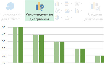
Функция Рекомендуемые диаграммы в приложении Excel предлагает вам типы диаграмм, лучше всего подходящие для введенных значений. Она позволяет просмотреть различные виды оформления и выбрать диаграмму на ваш вкус. Испытайте эту функцию в действии, чтобы создать диаграмму от начала до конца.

Использование срезов для фильтрации данных

Срезы впервые появились в Excel 2010 в качестве интерактивного способа фильтрации данных в сводных таблицах, а теперь их можно использовать и для фильтрации таблиц Excel, таблиц запросов и других типов таблиц. Срезы стало удобнее настраивать и использовать, так как они показывают текущий фильтр, что позволяет понять, какие именно данные отображаются.

Отдельные окна для книг

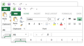
В Excel 2013 каждая книга отображается в отдельном окне, что облегчает одновременную работу с несколькими книгами. Это также помогает при работе с двумя мониторами.

Новые функции Excel

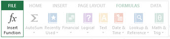
Были добавлены некоторые математические, тригонометрические, статистические и инженерные функции, функции для работы с датой и временем, ссылками, а также логические и текстовые функции. Также добавлены функции для работы с веб-службами REST. Дополнительные сведения см. в статье Новые функции Excel 2013.

Сохранение файлов и обмен ими в Интернете

Excel упрощает сохранение книг в сетевом расположении, например в бесплатной службе OneDrive или Microsoft 365 вашей организации. Также упрощен обмен листами с другими пользователями. Независимо от своего устройства и местоположения каждый пользователь работает с последней версией листа — возможна даже совместная работа в реальном времени.

Внедрение данных листа в веб-страницу

Для обмена листами в Интернете их можно внедрять в веб-страницы. После этого другие люди смогут работать с данными в Excel в Интернете открывать внедренные данные в Excel.

Обмен листами Excel в онлайн-встрече

Независимо от вашего местоположения и устройства (смартфона, планшета или ПК) с его помощью можно подключиться к онлайн-встрече и обмениваться книгами, если на нем установлено приложение Lync.

Сохранение файлов в новом формате

Теперь можно сохранять и открывать файлы в новом формате Strict Open XML Spreadsheet (XLSX). Он позволяет считывать и записывать даты в формате ISO8601, что устраняет проблему с ошибочной интерпретацией 1900 года как високосного. Дополнительные сведения см. в статье Сохранение книги в другом формате.

Новые функции для создания диаграмм

Изменения ленты диаграмм

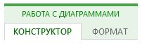
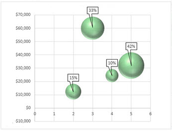
Новая кнопка Рекомендуемые диаграммы на вкладке Вставка помогает выбирать подходящий для данных тип диаграммы. Похожие типы диаграмм, например точечные и пузырьковые, теперь объединены в группы. Также добавлена кнопка для комбинирования диаграмм. При выборе диаграммы появляется упрощенная лента «Работа с диаграммами». В ней отображаются только вкладки Конструктор и Формат, что облегчает поиск нужных элементов.

Быстрая настройка диаграмм

Три новых кнопки позволяют быстро выбирать и просматривать изменения элементов диаграммы (например, заголовков или меток), ее внешнего вида и стиля или отображаемых данных. Подробнее об этом см. в элементах формата диаграммы.

Форматируемые метки данных

Теперь вы можете добавлять в метки данных форматируемый и обновляемый текст из точек данных и любой другой текст, настраивать их формат и отображать их в любом месте фигуры. Метки остаются на месте даже при изменении типа диаграммы. Их также можно соединить линиями выноски с соответствующими точками данных в любом типе диаграммы, а не только в круговом. Дополнительные сведения о работе с форматируемыми метками данных см. в статье Изменение формата меток данных в диаграмме.

Просмотр анимации в диаграммах

Диаграммы меняются при изменении исходных данных. Это делает внесение изменений не только интереснее, но и нагляднее.

Широкие возможности анализа данных

Создание подходящей сводной таблицы

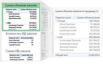
Выбор правильных полей для обобщения данных в отчете pivottTable может быть непростой задачей. Теперь вы можете получить помощь по этому. При создании таблицы Excel рекомендует несколько способов подведения итогов по данным и позволяет быстро просмотреть макеты полей, чтобы выбрать тот, который позволяет получить искомую информацию. Дополнительные сведения см. в теме «Создание таблицы для анализа данных на нем».

Создание различных типов сводных таблиц с помощью одного списка полей

С помощью одного списка полей можно создать макет сводной таблицы, в которой используется одна или несколько таблиц. Список полей, который теперь поддерживает как однотабличные, так и многотабличные сводные таблицы, упрощает поиск нужных полей в макете, переход на новую модель данных Excel с добавлением новых таблиц и навигацию по ним. Дополнительные сведения см. в статье Использование списка полей для упорядочения полей сводной таблицы.

Использование нескольких таблиц при анализе данных

Новая модель данных Excel позволяет использовать полезные функции анализа, ранее доступные только после установки надстройки Power Pivot. Помимо создания обычных сводных таблиц, теперь можно создавать сводные таблицы на базе нескольких таблиц Excel. Импортируя различные таблицы и создавая связи между ними, можно получать результаты анализа, недостижимые при использовании обычных сводных таблиц. Дополнительные сведения см. в статье Создание модели данных в Excel.

Power Query

Если вы используете Office профессиональный плюс 2013 или Приложения Microsoft 365 для предприятий, вы можете использовать Power Query для Excel. Она упрощает поиск информации в общедоступных и корпоративных источниках, а также подключение к ним. Это средство поддерживает новые способы поиска данных, а также функции для простого преобразования и слияния информации из нескольких источников для последующего анализа в Excel. Дополнительные сведения см. в статье Обнаружение и объединение данных с помощью Power Query для Excel.

Power Map

Если вы используете Приложения Microsoft 365 для предприятий, Office 2013 или Excel 2013, вы можете использовать Power Map для Excel. Power Map — это средство для трехмерной (3D) визуализации данных, позволяющее взглянуть на информацию под разными углами с использованием географических данных и параметров времени. Вы даже можете обнаружить тенденции, которые не смогли увидеть в традиционных двумерных (2D) таблицах и диаграммах. Надстройка Power Map встроена Приложения Microsoft 365 для предприятий, но для ее использования с Office 2013 или Excel 2013 необходимо скачать предварительную версию. Дополнительные сведения об этой пробной версии см. в статье Power Map для Excel. Дополнительные сведения об использовании Power Map для создания виртуальных трехмерных обзоров на основе выбранных данных см. в статье Приступая к работе с Power Map.

Подключение к новым источникам данных

Чтобы использовать несколько таблиц в модели данных Excel, теперь можно подключаться к дополнительным источникам данных и импортировать данные из них в Excel в виде обычных или сводных таблиц. Например, вы можете подключиться к таким источникам, как OData, Windows Azure DataMarket и источникам данных SharePoint. Также можно подключаться к источникам дополнительных поставщиков OLE DB.

Создание связей между таблицами

Если вы используете в своей модели данных Excel информацию из различных источников и нескольких таблиц, вы можете создать связи между ними, чтобы упростить анализ данных и избавиться от необходимости объединять их в одну таблицу. Запросы MDX позволяют создавать понятные отчеты сводных таблиц с применением таких связей. Дополнительные сведения см. в статье Создание связей между двумя таблицами.

Использование временной шкалы для отображения различных временных интервалов

Временная шкала упрощает сравнение данных из сводных таблиц или сводных диаграмм по временным интервалам. Вместо группирования по датам вы можете просто фильтровать даты или перемещаться между последовательными временными интервалами одним движением. Дополнительные сведения об этом см. в статье Создание временной шкалы сводной таблицы для фильтрации по дате.

Использование детализации, поднятия и перекрестного перехода между уровнями данных

Переход по уровням детализации в сложном наборе данных — непростая задача. Пользовательские наборы могут облегчить ее, но их поиск в списке полей занимает много времени. В новой модели данных Excel навигация по уровням упрощена. Команда Детализация позволяет подробнее изучить сведения, содержащиеся в сводной таблице или на сводной диаграмме, а команда Поднятие — перейти на более высокий уровень для оценки общей картины. Дополнительные сведения об этом см. в статье Изучение данных сводной таблицы на разных уровнях.

Использование вычисляемых компонентов и показателей OLAP

В данные сводной таблицы, подключенной к кубу OLAP, можно добавлять вычисления, основанные на MDX. Необязательно использовать модель объектов Excel — создавать показатели и вычисляемые компоненты и управлять ими можно непосредственно в Excel.

Создание автономной сводной диаграммы

Сводные диаграммы теперь не нужно связывать со сводными таблицами. Автономные и несвязанные сводные диаграммы поддерживают новые способы перехода между различными уровнями детализации благодаря новым функциям Детализация и Поднятие. Кроме того, несвязанные сводные диаграммы проще копировать и перемещать. Дополнительные сведения об этом см. в статье Создание сводной диаграммы.

Представление Power View

В наборе приложений Office профессиональный плюс есть представление Power View, которое вызывается с помощью соответствующей кнопки на ленте. Вы сможете взглянуть на свои данные под разными углами с помощью интерактивных, эффективных и удобных функций анализа, визуализации и представления информации. Представление Power View позволяет создавать и использовать диаграммы, срезы и другие средства визуализации данных на одном листе.

Новые и улучшенные надстройки и конвертеры

Power Pivot для надстройки Excel

Если вы используете Office профессиональный плюс 2013 или Приложения Microsoft 365 для предприятий, Power Pivot устанавливается вместе с Excel. В Excel теперь встроен модуль анализа данных Power Pivot, что позволяет создавать простые модели данных непосредственно в приложении. Power Pivot позволяет создавать более сложные модели. С ее помощью можно фильтровать данные при импорте, задавать собственные иерархии, поля вычислений и ключевые показатели эффективности (KPI), а также использовать язык выражений анализа данных (DAX) для создания сложных формул.

Надстройка Inquire

Если вы используете Office профессиональный плюс 2013 или Приложения Microsoft 365 для предприятий, надстройка Inquire устанавливается вместе с Excel. Она помогает анализировать и рецензировать книги, понимать их оформление, функции и зависимости между данными, а также обнаруживать различные проблемы, включая ошибки или несоответствия в формулах. Из надстройки Inquire можно запустить новое средство Microsoft Office под названием «Сравнение листов», позволяющее сравнить две версии книги, показывая изменения. Во время проверки видны все изменения, внесенные в книги.

Источник

Содержание

Что нового в Microsoft Excel 2013? [Обзор]
Земля в будущее
Время управлять аккаунтом и услугами
Документы везде
Конфиденциальность гарантирована
Путешествие от сохранения к обмену
Составление схемы вашего выхода
Анализировать данные в режиме реального времени, используя Быстрый анализ
Следуйте рекомендациям Excel
Поиск и вставка картинок онлайн
Офисные приложения: добраться до горизонта
Комплексные источники данных
Добраться до сути с Power View
Flash Fill: разумная организация ваших данных
решение суда
What’s new in Excel 2013
Top features to explore
Get started quickly
Instant data analysis
Fill out an entire column of data in a flash
Create the right chart for your data
Filter table data by using slicers
One workbook, one window
New Excel functions
Save and share files online
Embed worksheet data in a web page
Share an Excel worksheet in an online meeting
Save to a new file format
New charting features
Changes to the ribbon for charts
Fine tune charts quickly
Richer data labels
View animation in charts
Powerful data analysis
Create a PivotTable that suits your data
Use one Field List to create different types of PivotTables
Use multiple tables in your data analysis
Power Query
Power Map
Connect to new data sources
Create relationships between tables
Use a timeline to show data for different time periods
Use Drill Down, Drill Up, and Cross Drill to get to different levels of detail
Use OLAP calculated members and measures
Create a standalone PivotChart
Power View
New and improved add-ins and converters
Power Pivot for Excel add-in
Inquire add-in

Что нового в Microsoft Excel 2013? [Обзор]

Некоторые говорят, что Office 15 — просто отточенный вид предыдущей версии, но глубокий анализ Suite доказывает обратное. Да, времена меняются, и Microsoft адаптируется к новому миру, передав пользовательский интерфейс Metro, запущенный в Windows 8 и продолженный в новом предварительном просмотре Office. Обладая современным интерфейсом и удобной навигацией, облачные сервисы с использованием Microsoft SharePoint и SkyDrive позволяют вам работать как никогда. Кроме того, документы могут быть доступны на всех устройствах от мэйнфрейма до сенсорного телефона. Гладкое и отзывчивое рабочее пространство позволяет достичь производительности на новом пике. В этой статье мы расскажем о новых функциях Microsoft Excel 2013, начиная с новых параметров общего доступа и заканчивая приложениями Office. Организация данных была упрощена с помощью Flash Fill, анализ данных был оснащен Быстрый анализ и графики теперь намного эффективнее благодаря новым Рекомендуемые графики вариант.

Земля в будущее

Вместо того, чтобы открывать пустую электронную таблицу, чтобы задать поле для обширного сокращения чисел, Excel 2013 приветствует вас уникальной целевой страницей, которая позволяет вам понять актуальность этого приложения в организации каждого вопроса вашей жизни, от финансовых отчетов до личного бюджетирования, списки фильмов, анализ тенденций и многое другое. Они выложены перед вами в плиточном формате. Не забудьте нажать на шаблон «Добро пожаловать в Excel», чтобы быстро понять основы этой версии. Кроме того, панель поиска предлагает мощную синхронизацию с обновленной онлайн-библиотекой шаблонов Office. Вы можете быстро открыть часто используемые и последние использованные документы изпоследний Боковая панель.

Время управлять аккаунтом и услугами

Как вы, возможно, знаете, Excel 2013, как и другие инструменты в пакете Office, использует Live ID или учетную запись Microsoft SkyDrive для хранения контента в Интернете для лучшей доступности, совместного использования документов и совместной работы. Поэтому новый учетная запись На вкладке представлена информация о пользователях в сочетании с подключенными сервисами, организованными в три раздела: изображения и видео (Flickr, YouTube), хранилище (SharePoint, SkyDrive) и общий доступ. Кроме того, информация о продукте для общего набора представлен справа, с акцентом на подписку и обновления деталей. Новый интерфейс можно настроить с помощью Офисный фон темы.

Документы везде

В попытке сделать документы актуальными на ходу, окно «Открыть» в Excel 2010 было заменено целой страницей, охватывающей как онлайн, так и автономные места хранения. Вы можете открывать файлы из вашей системы или из вашего личного SkyDrive. Кроме того, Добавить местоПараметр позволяет указать другое местоположение SkyDrive и SharePoint, чтобы документы были доступны из любого места. Как видно, черты предыдущего последний Вкладка в Excel 2010 была объединена с новым открыто стр.

Конфиденциальность гарантирована

Новый Excel оценивает чувствительность ваших данных, особенно из-за уязвимостей, связанных с облачным хранилищем. Они преодолеваются пользовательскими настройками, такими как Проверять, выписываться функция, которая запрещает другим пользователям просматривать любые изменения или редактировать документ, если вы не предоставите им права редактирования. Более того, опции совместного использования защищают ваши данные в соответствии с вашими требованиями.

В Excel 2010 меню «Сохранить и отправить» было настолько богато, что оно не позволяло пользователям-новичкам вынудить их придерживаться нескольких кнопок в целях безопасности. Теперь вы можете получить доступ к этим опциям в очень организованной, удобной для пользователя форме с Поделиться, Сохранить как а также экспорт Вкладки. Важность командной работы и совместной работы никогда не следует игнорировать, особенно при работе с электронными таблицами, которые, как известно, охватывают широкий спектр материалов из различных источников. Иногда проблемы совместимости и прав являются препятствием для совместной работы над документом. Например, сотрудник может не иметь возможности просматривать документ Excel в полном объеме из-за старой версии Microsoft Excel. Вы можете не захотеть, чтобы другие редактировали окончательный документ, в то время как обратное должно относиться к вашему руководителю. Помня об этих проблемах, Excel 2013 предлагает несколько вариантов обмена.

После входа в свою учетную запись SkyDrive вы можете Приглашать людей указав их имена и адреса электронной почты в целях обмена. Вы можете дополнительно настроить интерфейс, включив или отключив процесс входа в систему. Кроме того, вы также можете создавать уникальные ссылки для обмена, которые можно ввести в браузер для полного доступа к документу, независимо от версии Excel, установленной на другом конце. Ссылки общего доступа классифицируются в форме просмотра ссылки (для общего доступа) и редактирования ссылки (для доступа администратора, позволяющего изменять права). Публичные ссылки также могут быть созданы путем активации соответствующей опции.

Чтобы указать сложные детали, касающиеся того, что общий зритель должен видеть в своем браузере, вы можете использовать новый Параметры просмотра в браузере в экспорт Вкладка. Это позволяет настроить рабочую книгу для соответствующего просмотра в Интернете.

Составление схемы вашего выхода

Самым впечатляющим дополнением к Microsoft Excel является новый и интерактивный способ работы с диаграммами. Важность Excel 2013 заключается в его аналитических возможностях и возможностях организации данных. Как только вы выберете диаграмму, элементы диаграммы кнопки всплывающих окон в правом верхнем углу. Все, что вам нужно сделать сейчас, это выбрать элементы, которые могут добавить больше значения к диаграмме, такие как Таблица данных, Строки ошибок, Временная шкала, Названия и многое другое.

Еще одна полезная кнопка, которая всплывает с графиком, это Стили диаграмм которые оснастят вас новым макетом и цветами. Эти стили и цвета обязательно сделают ваши графики, диаграммы и диаграммы более привлекательными для зрителя.

Еще одна впечатляющая особенность Фильтры диаграммы опция, которая выкладывает все переменные (серии) и категории для интерактивного просмотра. Просто наведите курсор на каждый элемент, и соответствующий контент на иллюстрации будет выделен. Теперь вы можете сосредоточиться на важных наборах данных, разложенных с течением времени, для более точного анализа.

Анализировать данные в режиме реального времени, используя Быстрый анализ

При работе с таблицами Быстрый анализ Кнопка позволяет анализировать данные из мощного набора форматирования, графиков, итогов, таблиц и Sparklines инструменты, которые мгновенно отображают результаты на вашем столе для мгновенного анализа. Добавить значение в столбцы таблицы никогда не было так просто.

Следуйте рекомендациям Excel

Вставить Вкладка Excel 2013 обладает множеством новых функций — от рекомендуемых сводных таблиц до рекомендуемых диаграмм. Цель 2013 — позволить вам добиться максимальных результатов за минимально возможное время. Для достижения наилучшего результата используйте эти рекомендации, чтобы определить и использовать сводные таблицы (инструмент суммирования данных) и диаграммы, которые лучше всего подходят для наложения данных на листе.

Поиск и вставка картинок онлайн

Вместо того, чтобы искать изображения онлайн с помощью поисковых систем, Excel 2013 предлагает вам возможность достичь этого, оставаясь при этом актуальным для рабочего листа. Бесплатную библиотеку фотографий, учетные записи Bing Image Search, учетные записи SkyDrive и Flickr можно использовать для поиска, предварительного просмотра и вставки соответствующих изображений в рабочее пространство.

Офисные приложения: добраться до горизонта

Когда вы подумали, что освоили Excel 2013, Office Apps сделает вас на шаг впереди. С полезными приложениями и обширной библиотекой ресурсов в Магазине Office, вы можете вставить интересные функции в свой рабочий лист. Следовательно, нет необходимости делать все самостоятельно, просто позвольте приложениям Office вывести вас за горизонт.

Комплексные источники данных

По сравнению с Excel 2010, новая версия предлагает обширный список источников данных, который умножает влияние вашей актуальности данных. В Excel 2013 предусмотрена возможность импорта данных в виде таблицы или сводной таблицы из Windows Azure Marketplace и канала данных ODATA. С исчерпывающими источниками данных вы можете легко отслеживать последние данные, относящиеся к вашим рабочим листам.

Добраться до сути с Power View

Надстройка Power View позволяет определять визуально привлекательные сводки вашего рабочего листа с особым акцентом на переменные, которые действительно важны для вас. С отдельной вкладкой у вас есть возможность просматривать данные так, как вам удобно. После определения соответствующих полей питания Power View извлекает информацию из выбранной рабочей таблицы, чтобы дать вам полный обзор указанных фильтров просмотра. Кроме того, вы можете выбрать новую тему, фон, прозрачность, изображения и другой контент со свободой эффективно вставлять, изменять, упорядочивать и анализировать отношения.

Flash Fill: разумная организация ваших данных

Новая захватывающая функция, которая обещает сэкономить ваше время и усилия, Flash Fill. Excel 2013 разумно использует шаблоны данных и тенденции, интерпретируя соответствующее значение, чтобы помочь вам в выполнении этой задачи. Например, после заполнения адресов электронной почты полными именами вы начинаете вводить имена в новом столбце, и, прежде чем вы узнаете его, Excel 2013 автоматически заполняет весь столбец. Теперь вы наверняка можете заполнить рабочий лист в одно мгновение!

решение суда

В целом, Microsoft Excel 2013 улучшил пользовательский интерфейс, сосредоточившись на флэш-заполнении, быстром анализе и интеллектуальных диаграммах. Теперь ваши данные находятся в гораздо лучшем положении, чтобы убедить и передать смысл соответствующим направлениям как в автономном, так и в онлайн-режиме. Необработанные данные теперь можно эффективно конвертировать с использованием рекомендуемых инструментов анализа данных и организации.

Источник

What’s new in Excel 2013

Note: SkyDrive is now OneDrive, and SkyDrive Pro is now OneDrive for Business. Read more about this change at From SkyDrive to OneDrive.

Tip: To learn how you can get started creating a basic Excel workbook quickly, see Basic tasks in Excel.

Top features to explore

Get started quickly

Templates do most of the set-up and design work for you, so you can focus on your data. When you open Excel 2013, you’ll see templates for budgets, calendars, forms, and reports, and more.

Instant data analysis

The new Quick Analysis tool lets you convert your data into a chart or table in two steps or less. Preview your data with conditional formatting, sparklines, or charts, and make your choice stick in just one click. To use this new feature, see Analyze your data instantly.

Fill out an entire column of data in a flash

Flash Fill is like a data assistant that finishes your work for you. As soon as it detects what you want to do, Flash Fill enters the rest of your data in one fell swoop, following the pattern it recognizes in your data. To see when this feature comes in handy, see Split a column of data based on what you type.

Create the right chart for your data

With Chart recommendations, Excel recommends the most suitable charts for your data. Get a quick peek to see how your data looks in the different charts, and then simply pick the one that shows the insights you want to present. Give this feature a try when you create a chart from start to finish.

Filter table data by using slicers

One workbook, one window

In Excel 2013 each workbook has in its own window, making it easier to work on two workbooks at once. It also makes life easier when you’re working on two monitors.

New Excel functions

Embed worksheet data in a web page

To share part of your worksheet on the web, you can simply embed it on your web page. Other people can then work with the data in Excel for the web or open the embedded data in Excel.

No matter where you are or what device you’re on—be it your smartphone, tablet, or PC—as long as you have Lync installed, you can connect to and share a workbook in an online meeting.

Save to a new file format

New charting features

Changes to the ribbon for charts

The new Recommended Charts button on the Insert tab lets you pick from a variety of charts that are right for your data. Related types of charts like scatter and bubble charts are under one umbrella. And there’s a brand new button for combo charts—a favorite chart you’ve asked for. When you click a chart, you’ll also see a simpler Chart Tools ribbon. With just a Design and Format tab, it should be easier to find what you need.

Fine tune charts quickly

Richer data labels

View animation in charts

See a chart come alive when you make changes to its source data. This isn’t just fun to watch—the movement in the chart also makes the changes in your data much clearer.

Powerful data analysis

Create a PivotTable that suits your data

Use one Field List to create different types of PivotTables

Use multiple tables in your data analysis

Power Query

Power Map

Connect to new data sources

Create relationships between tables

Use a timeline to show data for different time periods

Use Drill Down, Drill Up, and Cross Drill to get to different levels of detail

Drilling down to different levels of detail in a complex set of data is not an easy task. Custom sets are helpful, but finding them among a large number of fields in the Field List takes time. In the new Excel Data Model, you’ll be able to navigate to different levels more easily. Use Drill Down into a PivotTable or PivotChart hierarchy to see granular levels of detail, and Drill Up to go to a higher level for “big picture” insights. To learn more about it, see Drill into PivotTable data.

Use OLAP calculated members and measures

Create a standalone PivotChart

A PivotChart no longer has to be associated with a PivotTable. A standalone or de-coupled PivotChart lets you experience new ways to navigate to data details by using the new Drill Down, and Drill Up features. It’s also much easier to copy or move a de-coupled PivotChart. To learn more about it, see Create a PivotChart.

Power View

New and improved add-ins and converters

Power Pivot for Excel add-in

Inquire add-in

Источник

Top features to explore
- Get
  started quickly
- Instant data analysis
- Fill
  out an entire column of data in a flash
- Create
  the right chart for your data
- Filter
  table data by using slicers
- One workbook, one window
- New
  Excel functions
- Save and share files online
- Embed worksheet data in a web page
- Share an Excel worksheet in an online meeting
- Save to a new file format
New charting features
- Changes to the ribbon for charts
- Fine tune charts quickly
- Richer data labels
- View animation in charts
Powerful data analysis
- Create
  a PivotTable that suits your data
- Use one Field List to create different types of PivotTables
- Use multiple tables in your data analysis
- Connect to new data sources
- Create relationships between tables
- Use a timeline to show data for different time periods
- Use Drill Down, Drill Up, and Cross Drill to get to different levels
  of detail
- Use OLAP calculated members and measures
- Create a standalone PivotChart
- Power View
New and improved add-ins and converters
- PowerPivot for Excel add-in
- Inquire add-in

View
the video that shows the new features.

The first thing you’ll see when you open Excel is a brand new look. It’s cleaner, but it’s also designed to help you get professional-looking results quickly. You’ll find many new features that let you get away from walls of numbers and draw more persuasive
pictures of your data, guiding you to better, more informed decisions.

Tip To learn how you can get started creating a basic Excel workbook quickly, see

Basic tasks in Excel 2013.

Top features to explore

Get
started quickly

Templates do most of the set-up and design work for you, so you can focus on your data. When you open Excel 2013, you’ll see templates for budgets, calendars, forms, and reports, and more.

Instant data analysis

Fill
out an entire column of data in a flash

Flash Fill is like a data assistant that finishes your work for you. As soon as it detects what you want to do,
Flash Fill enters the rest of your data in one fell swoop, following the pattern it recognizes in your data. To see when this feature comes in handy, see

Split a column of data based on what you type.

Create
the right chart for your data

With Chart recommendations, Excel recommends the most suitable charts for your data. Get a quick peek to see how your data looks in the different charts, and then simply pick the one that shows the insights you want to present.
Give this feature a try when you
create your first chart.

Filter
table data by using slicers

One workbook, one window

In Excel 2013 each workbook has in its own window, making it easier to work on two workbooks at once. It also makes life easier when you’re working on two monitors.

New
Excel functions

You’ll find several new functions in the math and trigonometry, statistical, engineering, date and time, lookup and reference, logical, and text function categories. Also new are a few Web service functions for referencing existing Representational State
Transfer (REST)-compliant Web services. Look for details in
New functions in Excel 2013.

Save and share files online

Excel makes it easier to save your workbooks to your own online location, like your free SkyDrive or your organization’s Office 365 service. It’s also simpler to share your worksheets with other people. No matter what device they’re using or where they are,
everyone works with the latest version of a worksheet— and you can even work together in real time. To learn more about it, see

Save a workbook to another location or
Save a workbook to the Web.

Embed worksheet data in a web page

To share part of your worksheet on the web, you can simply embed it on your web page. Other people can then work with the data in Excel Web App or open the embedded data in Excel.

Share an Excel worksheet in an online meeting

No matter where you are or what device you’re on—be it your smartphone, tablet, or PC—as long as you have Lync installed, you can connect to and share a workbook in an online meeting. To learn more about it, see

Present a workbook online.

Save to a new file format

Save a workbook in another file format.

Top of Page

New charting features

Changes to the ribbon for charts

The new Recommended Charts button on the
Insert tab lets you pick from a variety of charts that are right for your data. Related types of charts like scatter and bubble charts are under one umbrella. And there’s a brand new button for combo charts—a favorite chart you’ve asked for. When you
click a chart, you’ll also see a simpler Chart Tools ribbon. With just a
Design and Format tab, it should be easier to find what you need.

Fine tune charts quickly

Three new chart buttons let you quickly pick and preview changes to chart elements (like titles or labels), the look and style of your chart, or to the data that is shown. To learn more about it, see

Format your chart.

Richer data labels

Now you can include rich and refreshable text from data points or any other text in your data labels, enhance them with formatting and additional freeform text, and display them in just about any shape. Data labels stay in place, even when you switch to
a different type of chart. You can also connect them to their data points with leader lines on all charts, not just pie charts. To work with rich data labels, see

Change the format of data labels in a chart.

View animation in charts

See a chart come alive when you make changes to its source data. This isn’t just fun to watch—the movement in the chart also makes the changes in your data much clearer.

Top of Page

Powerful data analysis

Create
a PivotTable that suits your data

Picking the right fields to summarize your data in a PivotTable report can be a daunting task. Now you can get some help with that. When you create a PivotTable, Excel recommends several ways to summarize your data, and shows you a quick preview of the field
layouts so you can pick the one that gives you the insights you’re looking for. To learn more about it, see

Create a PivotTable.

Use one Field List to create different types of PivotTables

Create the layout of a PivotTable that uses one table or multiple tables by using one and the same Field List. Revamped to accommodate both single and multi-table PivotTables, the Field List makes it easier to find the fields you want in your PivotTable
layout, switch to the new Excel Data Model by adding more tables, and explore and navigate to all of the tables. To learn more about it, see

Learn how to use the Field List.

Use multiple tables in your data analysis

create PivotTables based on multiple tables in Excel. By importing different tables, and creating relationships between them, you’ll be able to analyze your data with results you aren’t able to get from traditional PivotTable data. To learn more about it,
see
Create a Data Model in Excel.

Connect to new data sources

To use multiple tables in the Excel Data Model, you can now connect to and import data from additional data sources into Excel as tables or PivotTables. For example, connect to data feeds like OData, Windows
Azure DataMarket, and SharePoint data feeds. You can also connect to data sources from additional OLE DB providers.

Create relationships between tables

When you’ve got data from different data sources in multiple tables in the Excel Data Model, creating relationships between those tables makes it easy to analyze your data without having to consolidate it into one table. By using MDX queries, you can further
leverage table relationships to create meaningful PivotTable reports. To learn more about it, see

Create a relationship between two tables.

Use a timeline to show data for different time periods

A timeline makes it simpler to compare your PivotTable or PivotChart data over different time periods. Instead of grouping by dates, you can now simply filter dates interactively or move through data in sequential time periods, like rolling month-to-month
performance, in just one click. To learn more about it, see
Create a PivotTable timeline to filter dates.

Use Drill Down, Drill Up, and Cross Drill to get to different levels
of detail

Drilling down to different
levels of detail in a complex set of data is not an easy task. Custom sets are helpful, but finding them among a large number of fields in the
Field List takes time. In the new Excel Data Model, you’ll be able to navigate to different levels more easily. Use
Drill Down into a PivotTable or PivotChart hierarchy to see granular levels of detail, and
Drill Up to go to a higher level for “big picture” insights. To learn more about it, see

Drill into PivotTable data.

Use OLAP calculated members and measures

Tap
into the power of self-service Business Intelligence (BI) and add your own Multidimensional Expression (MDX)-based calculations in PivotTable data that is connected to an Online Analytical Processing (OLAP) cube. No need to reach for the Excel Object Model—now
you can create and manage calculated members and measures right in Excel.

Create a standalone PivotChart

A PivotChart no longer has to be associated with a PivotTable. A standalone or de-coupled PivotChart lets you experience new ways to navigate to data details by using the new
Drill Down, and Drill Up features. It’s also much easier to copy or move a de-coupled PivotChart. To learn more about it, see

Create a PivotChart.

Power View

If you’re using Office Professional Plus, you can take advantage of Power View. Simply click the Power View button on the ribbon to discover insights about your data with highly interactive, powerful data exploration, visualization, and presentation features
that are easy to apply. Power View lets you create and interact with charts, slicers, and other data visualizations in a single sheet. Learn more about

Power View in Excel 2013.

Top of Page

New and improved add-ins and converters

PowerPivot for Excel add-in

If you’re using Office Professional Plus, the PowerPivot add-in comes installed with Excel. The PowerPivot data analysis engine is now built into Excel so that you can build simple data models directly in Excel. The PowerPivot add-in provides an environment
for creating more sophisticated models. Use it to filter out data when importing it, define your own hierarchies, calculation fields, and key performance indicators (KPIs), and use the Data Analysis Expressions (DAX) language to create advanced formulas. Learn
more about the
PowerPivot in Excel 2013 add-in.

Inquire add-in

If you’re using Office Professional Plus, the Inquire add-in comes installed with Excel. It helps you analyze and review your workbooks to understand their design, function, and data dependencies, and to uncover a variety of problems including formula errors
or inconsistencies, hidden information, broken links and others. From Inquire, you can start a new Microsoft Office tool, called Spreadsheet Compare, to compare two versions of a workbook, clearly indicating where changes have occurred. During an audit, you
have full visibility of the changes in your workbooks.

Источник

As you may new, the newest version of Excel is out for a while. I have been using it since last 6 months and enjoying it. Today, lets understand 10 things in 2013 that wowed me (and probably you too).

Flash Fill

Imagine Flash (the super hero, not browser add-in) is using Excel to extract the middle names of all his villains. Now, flash being flash, do you think he will slowly type out the middle names one at a time? Of course, he can learn Excel formulas and do it in one stroke. But he is too busy running around & saving earth. So, obviously he would use Flash Fill.

Flash Fill works almost like magic. It looks at what you are typing and sees if there is any pattern in it (based on adjacent columns etc.) and then suggests a fill down option. See this demo.

Bonus Tip: Press CTRL+E to activate flash fill.

Built-in Data Model

The top 3 reasons why analysts & managers spend so much time with Excel:

Searching for that mysterious flight simulator Easter egg (#)
Formatting worksheets
Trying to link up multiple tables of data using VLOOKUP, Copy Paste and black magic.

Fortunately Excel 2013 makes #3 a breeze, thanks to built-in data model. Using Excel 2013 data model, you can link multiple tables with each other (one to one or one to many relationships) and generate powerful Pivot reports & charts with few clicks. Now you have more time to search for flight simulator.

Timelines

These days everybody boasts of a massive spreadsheet. But almost no one needs all the data at same time. We are always filtering data for latest quarter, 6 months starting Mother’s day or 8 weeks from November 1st etc. Of course, you can use auto-filter and select all the dates. But it is a pain.

Thanks to Timelines, filtering for dates is a breeze. You can add timelines for any date column in a pivot table / pivot chart. I am sure your clients & bosses will love it.

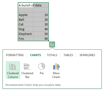
Quick Analysis

Depending on your work, you may love or hate it. Quick analysis is a new button that appears when you select a bunch of data. Using this, you can do a lot of quick analysis tasks like adding conditional formatting, charts, sparklines or turning your data in to tables (or pivots). To be frank, I find this a bit of annoyance as my analysis work is never quick!

But I am sure there are tons of people who would find this very useful.

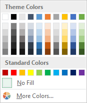
Excellent color scheme

The default color scheme of Excel 2013 is bold, creative and well contrasted. It is a far cry from Excel 2003’s color scheme (which is boring, glaring & poorly contrasted). Now, if you insert a default chart (or table, pivot etc.) from your data, you need to do very little clean up work. It is ready to go!!!

Distinct Counts & more in your Pivot

If you are really quiet, you can hear an analyst in your company screaming with joy once they realize that in Excel 2013, you can get distinct count of values in pivot reports!!!

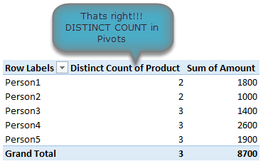
That is right, using Excel 2013 pivot reports, you can find out distinct counts. No extra formulas or no arrays or no VBA. More power to you 🙂

[Related: Using Distinct Count feature in Excel 2013 – case study]

New Formulas

In Excel 2013, there are many new formulas and improvements. My favorite new formulas are,

Web formulas – WEBSERVICE(), FILTERXML() and ENCODEURL() (an example on these formulas)
Information formulas – ISFORMULA(), FORMULATEXT(), SHEET() and SHEETS()
Logical – XOR(), IFNA(), BITXOR(), BITOR(), BITAND() etc.

Easier Charting

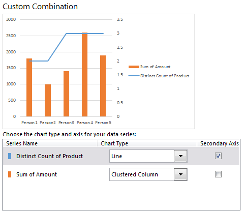
In Excel 2013, there are massive changes in charting. Now you can create combination charts, add secondary axis, set up smart data labels, format the chart or switch styles with ease. Microsoft revamped the default formats too so that when you make a chart from data, it is ready for presentation (with out too many tweaks).

Some of favorite charting features are,

Recommended charts feature that tells you which charts go well with your data.
A screen where you can change the chart type for each series easily.
Common chart customizations are a click away (screenshots 1, 2 & 3)
Ability to create scatter plots based on a variety of input data layouts (Jon Peltier’s article on this).

That said not everything is rosy with 2013 charting. For example, I do not like that we have to go thru sidebar pane to customize charts (formatting etc.) instead of dialog box.

Animated Charts

One of the slickest things you will notice in Excel 2013 is the animation that you see when you move selection, do calculations or create charts. While this may be annoying to some, I find one good use for it. When you use charts coupled to interactive elements (like form controls, slicers etc.) they look sexier, thanks to Animation. See this demo to understand what I mean.

Power to you

Excel 2013 Professional Plus versions comes bundled with Power Pivot & Power View, 2 excellent features for powerful data analysis & visualization. You can think of these as full fledged BI solutions sitting right in your computer. The only glitch, Microsoft decided to give these features only Professional Plus users. I know it is annoying that home, office, professional level licenses cannot use Power Pivot even if they want to pay extra. What a pity!!!

More on Excel Power Pivot licensing issues & possible solutions.

Related: What is PowerPivot & How to use it?

3 things that are not so impressive

The whole cloud thing:

While it is understandable that Microsoft wants us all to purchase shiny new Surface tablets and use spreadsheets on the go, it seems like a bad idea. It annoys me that when I want to save a file, the first option I see is Chandoo’s sky drive. The process of saving files to sky drive and later viewing them in browsers is very slow and often results in errors or warnings. Instead, for desktop versions, why not make My computer as first preference?!?

Sharing & Social features:

Share to Facebook?!? seriously! Why would anyone want to share their spreadsheets on twitter or facebook? Do we really want facebook to know our annual budget & appraisal ratings (so that they can show us ads that say – Buy our scissors and cut your budget in half )?

Power Pivot is not for masses:

Microsoft positioned Power Pivot as BI for masses, offered it for free in Excel 2010. Then in Excel 2013, they went ahead and implemented a licensing policy that looks just as complicated as my lawyer’s invoice. Why would a for-profit company like MS want to not offer powerful tools like Power Pivot to masses for a fee? Why sell it only to corporate customers thru volume licensing program? beats me.

Bottom line

Despite these minor annoyances, I think Excel 2013 is a well designed, solid & powerful software ready to make more people awesome in their work. With features like tablet compatibility, data model, slicers & timelines, improved UI & color schemes it has quickly become my first choice when I want to use a spreadsheet (I run Excel 2010 & 2013 on same computer).

Are you using Excel 2013, what do you like about it?

Are you using Excel 2013? How do you like it? Which features are best according to you? Please share your thoughts and views using comments.

Share this tip with your colleagues

Excel and Power BI tips - Chandoo.org Newsletter

Get FREE Excel + Power BI Tips

Simple, fun and useful emails, once per week.

Learn & be awesome.

48 Comments
Ask a question or say something…
Tagged under

animation, auto fill, charting, combination charts, data model, distinct count, excel 2013, flash fill, Learn Excel, list posts, powerpivot, quick analysis, timelines
Category:

Charts and Graphs, Learn Excel

Welcome to Chandoo.org

Thank you so much for visiting. My aim is to make you awesome in Excel & Power BI. I do this by sharing videos, tips, examples and downloads on this website. There are more than 1,000 pages with all things Excel, Power BI, Dashboards & VBA here. Go ahead and spend few minutes to be AWESOME.

Read my story • FREE Excel tips book

Excel School made me great at work.

 5/5

Excel formula list - 100+ examples and howto guide for you

From simple to complex, there is a formula for every occasion. Check out the list now.

Calendars, invoices, trackers and much more. All free, fun and fantastic.

Power Query, Data model, DAX, Filters, Slicers, Conditional formats and beautiful charts. It’s all here.

Still on fence about Power BI? In this getting started guide, learn what is Power BI, how to get it and how to create your first report from scratch.

Related Tips

48 Responses to “10 things that wowed me in Excel 2013”

In general I don’t dislike Excel 2013. The stark white interface took some adjustment, and the all caps ribbon tab labels bugged me until I realized I could change them. And continuing a trend, we lose a row or two from the full screen worksheet.
There have in fact been many improvements to charting in 2013.
The recommended charts feature is so-so, partly because of all of the ineffective chart types that have been baked into Excel.
2/3 of the icons that appear next to the active chart are awesome. The plus sign icon that lets you add elements without a long journey to the ribbon: awesome, if a step back to 2003. The filtering capabilities that let you on the fly hide series or points without mucking with the worksheet: double awesome. The style paintbrush suffers from the same problems of the styles on the ribbon: too much over-the-top gratuitous formatting.
You know you can grab the title bar of the task pane and drag it away from its docked position? Now it floats wherever you want it. The task pane/dialog is painful to navigate, though, with too much scrolling, and the item you want is always hidden behind a click to activate or expand its category or to expand
The animation of chart changes is annoying at best, distracting and confusing at worst.
Also, I seem no longer to be able to edit a series formula in the formula bar.
- B-Dog says:
  
  No one has mentioned one of the best things about 2013. On dual monitors, I don’t have to create a second instance to have an Excel spreadsheet open on each screen. I can drag a file to the other monitor opened in the same instance, fixing all those copy- paste issues or moving tabs from one file to another.
John Jingle says:

I’m still using Excel 2003. I tried 2007 and it is absolute garbage.
I hear good things about 2010 and am hearing really good things about 2013.

Is it worth it to make the switch from 2003 to 2013 or would 2010 be better?
- zx8754 says:
  
  Either of them will give you «Ribbon shock effect» related headaches…
I really liked the improved Flash Fill feature in Excel 2013. Another nice feature in Excel 2013 is that it allows multiple collaborators to edit a single worksheet simultaneously.
Harish says:

I am agree with John Jingle…. as still I am also useing Excel 2003 becouse of lots issue with excel charting and ribbon. Jon is also right ribbon grabs one and two row of full screen excel. but we can’t avoid advance fature of excel 2007,2010 and 2013. I am also not agree with chandoo’s line «No extra formulas or no arrays or no VBA». The value of VBA and advance function know only a good Excel Developer who can do anything in 2003 also which is in excel 20013 and 2010 with the help of APIs.
Wookiee says:

Did the Flash Fill feature actually work correctly in the demo above? To me, the sequence that it should have produced was the first letter of each new word in the adjacent cell, but the sequence it came up with was merely the first letter in the cell doubled.
Either way, «Captain Cold» and «Gorilla Grodd» would produce the same initials, but «Professor Zoom» was PP instead of PZ and Captain Boomerang was CC instead of CB.
Does Flash Fill default to the first pattern it identifies, or does it offer alternate patterns if you determine that it is not correctly identifying the nature of your intended fill?
- You are right. I did not notice it. That said, Flash fill assumes the pattern based on what you input in first few cells. So I kind of misled it. 🙂
  - HARESH SHRIMALI says:
    
    Yes, Chandoo, Excel 2013 doesn’t like our RAHUL GANDHI , it gave me RJ &
    it doesn’t at all like our Priyanka Gandhi, it gave me PZ & in my case,
    for Professor Zoom it gave correct PZ .Professor Zoom — PP, Ramesh Jadeja-RR , Arvind Kezriwal-AA, Captain Boomerang-CC, Rahul Gandhi-RR, Menka Gandhi-MM, Priyanka Gandhi-PP, Soniya Gandhi — SS, Professor Zoom-PP . SO , Chandoo, Must I jump to the Final Conclusion that Excel 2013 Flash Feature doesn’t like our Politicians, particularly Gandhi-Nehru Parivar? Ha Ha ha. !!!! Is it called a bug in Excel 2013 , Chandoo ?
    - Carol says:
      
      I typed in the list above and hit enter when it suggested the list you have above. As soon as I was done with that, Arrowed down to the cell that had PP instead of PZ. I typed in PZ and it fixed the pattern for the rest of the column. Got the appropriate first and last initial for the rest of the list.
  - But Chandoo & my Guru, I noticed quite significant CORRECTNESS IN EXCEL 2013, & you are Absolutely Correct Chandoo, Excel 2013, adjusts all second raw onwards, evenif I wrote long Names like
    
    Haresh Jagjivan Shrimali
    
    Chandoo P Godzilla
    
    Chanakya G Einstein
    
    Ramesh Pranlal Jadeja
    
    Arvind G Kezriwal
    
    Professor B Zoom
    
    Rahul R Gandhi
    
    Menka Sanjay gandhi
    
    Priyanka T Gandhi
    
    Soniya Rajiv Gandhi
    
    Professor Kanji Zoom
    
    Haresh Jagjivan Shrimali it gave 100% correct Flash Filling from third raw onwards, it gave 100% Correct Result! Amazing Microsoft, Chandoo & my Guru.
Steve Farrar says:

I found that certain macros run much slower in 2013 and seems to crash a bit more than 2010- other than that it’s ok
Kyle says:

This is not about excel, but I enjoy reading your emails because you put a great sense of humor in a topic that can be dry at time 🙂
Swapnil says:

Hey Chandoo,

Nice points. Its worth reading humored blogs, than referring MS site.

Thanks
I am yet to use Excel 2013.In fact till few days back I was using 2007 and very recently switched to 2011 version. Now after reading the article I can’t wait to grab 2013 version.
- hamad says:
  
  2011? for mac? there is no 2013 for mac!
Frank Linssen says:

It is good to read that you have 2010 and 2013 installed on your computer both.
I was not sure this was possible.
Did you need to do something fancy to have it installed next to your 2010 version or is it just a question during installation?
Regards
- During installation you have a choice to «upgrade office» or «install office». Choose install. This will keep older versions intact. Please note that Outlook will be upgraded no matter what.
  - Frank Linssen says:
    
    I bought the 64 bit version to be ibstalled on my Windows 7 computer.
    To my surprise, Office asked me to first uninstall the older versions before I was allowed to install the new version 2013. As I want to keep my older versions too I haven’t installed it.
    Did anybody else face the same issue and how did you resolve it?
    ( it is already some time ago, but I think it also mentioned that I then have to install the 32bit version if I want to keep the older versions too on my computer)
    - Lou Barletta says:
      
      What worked for me in the past was to: 1) uninstall the old version, 2) install the new version, 3) reinstall the old version.
Thanks for this great post Chandoo! I am sure more than 75% of excel users can’t even use the complete features of Excel 2003 — the new 2013 version is new elite product for them 🙂
By the way how do you create animated GIFs? Like the one you did to show Animated Charts?
SIVAKUMAR R says:

Now only I use ms office 2010 I am waiting to use 2013 very soon
Gleb says:

I’ve sent that article to my boss and crossed my fingers. He MUST purchase new office after reading)))
Dear Chadooji and my Guruji

first of all I will appreciate for your works towards excel. I am fond of excel works. Daily I used to search for a new thing in excel.

I have seen Excel 2013, in which the new things are amazing.

Thanks to be a part of the team.

T/R
Satyanarayana
rahul aggarwal says:

like to see 10 great things in excel2013
but i am very eager and complaining to excel2013 about one (-ve) thing in excel2013
that is you can’t use ctrl+alt+F5 for refresh all pivot tables
if there is any other option please help
rvltn says:

Any chance of getting the new color scheme for my Excel 2007 (without defining every color on my own)?
Sharon says:

I am using Excel 2013 on Windows 8. How do I get Excel 2013 to show at the bottom of the screen all the files that are open just like in earlier versions of Excel? At the moment when in Excel 2013, I cannot see at a glance all the files I have opened unless I hover on the Excel pin/icon at the bottom of the screen. Thanks.
Brian says:

Waiiiiiiiiiiiiiiiiiit a minute…..

Does this mean there is no point learning Power Pivots if they are not available to most users? How much does a commercial license cost?
Furthermore, if you do have Power Pivot and you create a model for a client who doesn’t have Power Pivot in their version, does this mean that section of the model won’t be operational?
Oli says:

I’m sticking with 2010 as you get to keep PowerPivot and the new stuff in 2013 sees a little gimmicky?
Ryan says:

Chandoo how could you miss the biggest benefit of all…all workbooks open in their own window now!!!

Another annoyance I have is that when you hide columns on a dashboard (everything to the right of a column for example), 2013 still shows a white sheet instead of grey like in old versions. I like the previous way so that it looked like the dashboards were a little 3d.
mike says:

All I can say is… about bloody time.

I’ve been using a bitAND plug in for ages. Question is when will M$ allow the following

FFTs of vales not equal to 2^N and greater than 8192 long.
HEX2BIN and BIN2HEX of 32 and 64 bit values, ideally 128 bits or more.

And if they want to make all my macros run slower.. then they’ve just lost a sale (I suspect the comments here are from people who leave screen updates on while macros run.. lots of high level code will alway run ssssssssslllllllllllllllllloooooooooooowwwwwwwwww)

viva-assembly!

mike
using W7 hacked to make it play like 2000
excel 2010 with 2003 menus.
Tom says:

How about the feature where Excel crashes if you try to copy the results of a filtered table to another spreadsheet. That’s a great feature :(. It’s done it to me twice already and I’ve only been using it for a few days
- David says:
  
  You know, it hadn’t occurred to me that it was the fact that it was filtered that kept causing the crash. You might well have saved the last remaining strands of hair I had left on my head, Tom.
  
  I spent a maddening half day with constant crashing trying to incorporate a linked filtered data sheet into another file.
  
  Annoying to note that this is more than 6 months on from when you posted the issue …
Koos van Strien says:

Two things that annoy me:
— when I have a worksheet with the same name as an Excel function (which isn’t unlikely, take for example ‘Date’), I cannot use the DATE function anymore, because Excel auto-corrects the casing and sees it as my pivot table. When I rename the Excel worksheet to a normal name after that, Excel keeps auto-correcting the function to the sheet (which doesn’t exist any more) thus leaving me without a DATE function.
— When I have a Pivot Chart, I can’t set up an axis as a date axis, it always displays as a categorical axis. Maybe this is because of my local settings, and it works well in US, but it surely doesn’t in Dutch.
- Mark Schreiber says:
  
  I learned early to avoid using existing function names for variables. For example, use Mon instead of Month, Yr instead of Year, Dt instead of Date. This is especially important when using VBA.
Sonia says:

Great comments and thanks for summarising what’s new in 2013. I’ve been using it for a couple of months — my biggest gripe is the colour scheme — the choice of «light grey», «grey» or «dark grey» is annoying. This might be a Windows 8 problem — not sure. I work on Excel upto 8 hours — grey and white becomes very tiring on the eyes — I need to have a bit of colour. Would love to change the ribbon/tab colour.
manu says:

Hi Chandoo ji

My Excel 2013 keeps on crashing when I use solver add-in. Unfortunately I need to use the solver to do what I need to do by this in the next 2 days so disabling add-ins doesn’t really help.

I am just going through endless cycles of MS excel crashing and a message saying excel restarting then typing in a few char and going thru the same cycle again.

The machine is a Windows 7 machine with the necessary reqs needs for the install, only thing I can think of is maybe I installed it as 32-bit, instead of a 64-bit installation (as the Installer suggested).

Any suggestions.
Thanks

Manu
One aspect of 2013 that seem very interesting, although I haven’t put it to great effect, is the facility to «Drill down» with the Quick Explore button (only available for Data Model and cube data on pivot tables — that are hierarchical ). at first I thought it just added filters, but it seems to shift you column and rows around depending on what you drill into. Anyone found this feature useful ?
Danielle says:

I’m not extremely well-versed in excel but I’m still having difficulties locating where the display equation and display r-squared value options are.
Dan Alameda says:

As a whole, I do not like 2013. the extra steps to open a file, the inability to open two instances of Excel at once (or I just haven’t figured out how to do it yet), etc. It also seems to calculate changes slower than the other versions. There are some good points with it, for sure. Improved graphing capabilities, Sparklines (I skipped Excel 2010)
chessman says:

I have tried many pages with this list of news on excel, this is by far the best
congratulations and thanks
Vasanth Kumar says:

Hi can you please help me sum values as 02 x 40′ cell A and 04 x 40′ cell B which is in 2 different cells
VivekD says:

If I create a chart in Excel 2013 having the animated feature, would it work in Excel 2010 or lower versions?
- @VivekD
  
  No, Those animations only work in 2013
  
  Animations done with VBA will work in 2007+
Mark Schreiber says:

I agree with Dan, Excel 2013 seems a bit clumsy with opening files. I used to have a «Open Recent» icon on my Quick Tool Bar but it has disappeared. To me that is reducing capability. Opening multiple files must be done within Excel through the File/Open and the annoying step immediately after.

My first Excel version was 2.0 and I have used all of the versions between. 2013 us really…really…what’s the word…STUPID. Horrible colors, clunky icons. I wonder if Microsoft is setting us up for the next version, thinking we will gladly jump into the next version to get away from 2013.

At least my macros still work. I have not jumped into the VBA editor yet. I hope that experience is not unpleasant also.
[…] The ultimate goal of your excel worksheet is to present information in a way others will understand, right? Give readers a head start by titling your worksheet clearly. A good title lets readers know immediately what the content of the worksheet is going to show them — that way, they won’t have to work so hard. “2015 Projections” isn’t bad, but it leaves a lot of things out. What kind of projections? Sales? Hired Employees? New Store Openings? Be as clear as you can and, if necessary, add a subtitle. And if you plan to circulate the worksheet by e-mail, be sure that you title the worksheet file with something that reflects the content of the sheet itself. […]

Источник