
If you’re new to Excel for the web, you’ll soon find that it’s more than just a grid in which you enter numbers in columns or rows. Yes, you can use Excel for the web to find totals for a column or row of numbers, but you can also calculate a mortgage payment, solve math or engineering problems, or find a best case scenario based on variable numbers that you plug in.
Excel for the web does this by using formulas in cells. A formula performs calculations or other actions on the data in your worksheet. A formula always starts with an equal sign (=), which can be followed by numbers, math operators (such as a plus or minus sign), and functions, which can really expand the power of a formula.
For example, the following formula multiplies 2 by 3 and then adds 5 to that result to come up with the answer, 11.
=2*3+5
This next formula uses the PMT function to calculate a mortgage payment ($1,073.64), which is based on a 5 percent interest rate (5% divided by 12 months equals the monthly interest rate) over a 30-year period (360 months) for a $200,000 loan:
=PMT(0.05/12,360,200000)
Here are some additional examples of formulas that you can enter in a worksheet.
-
=A1+A2+A3 Adds the values in cells A1, A2, and A3.
-
=SQRT(A1) Uses the SQRT function to return the square root of the value in A1.
-
=TODAY() Returns the current date.
-
=UPPER(«hello») Converts the text «hello» to «HELLO» by using the UPPER worksheet function.
-
=IF(A1>0) Tests the cell A1 to determine if it contains a value greater than 0.
The parts of a formula
A formula can also contain any or all of the following: functions, references, operators, and constants.

1. Functions: The PI() function returns the value of pi: 3.142…
2. References: A2 returns the value in cell A2.
3. Constants: Numbers or text values entered directly into a formula, such as 2.
4. Operators: The ^ (caret) operator raises a number to a power, and the * (asterisk) operator multiplies numbers.
Using constants in formulas
A constant is a value that is not calculated; it always stays the same. For example, the date 10/9/2008, the number 210, and the text «Quarterly Earnings» are all constants. An expression or a value resulting from an expression is not a constant. If you use constants in a formula instead of references to cells (for example, =30+70+110), the result changes only if you modify the formula.
Using calculation operators in formulas
Operators specify the type of calculation that you want to perform on the elements of a formula. There is a default order in which calculations occur (this follows general mathematical rules), but you can change this order by using parentheses.
Types of operators
There are four different types of calculation operators: arithmetic, comparison, text concatenation, and reference.
Arithmetic operators
To perform basic mathematical operations, such as addition, subtraction, multiplication, or division; combine numbers; and produce numeric results, use the following arithmetic operators.
|
Arithmetic operator |
Meaning |
Example |
|
+ (plus sign) |
Addition |
3+3 |
|
– (minus sign) |
Subtraction |
3–1 |
|
* (asterisk) |
Multiplication |
3*3 |
|
/ (forward slash) |
Division |
3/3 |
|
% (percent sign) |
Percent |
20% |
|
^ (caret) |
Exponentiation |
3^2 |
Comparison operators
You can compare two values with the following operators. When two values are compared by using these operators, the result is a logical value — either TRUE or FALSE.
|
Comparison operator |
Meaning |
Example |
|
= (equal sign) |
Equal to |
A1=B1 |
|
> (greater than sign) |
Greater than |
A1>B1 |
|
< (less than sign) |
Less than |
A1<B1 |
|
>= (greater than or equal to sign) |
Greater than or equal to |
A1>=B1 |
|
<= (less than or equal to sign) |
Less than or equal to |
A1<=B1 |
|
<> (not equal to sign) |
Not equal to |
A1<>B1 |
Text concatenation operator
Use the ampersand (&) to concatenate (join) one or more text strings to produce a single piece of text.
|
Text operator |
Meaning |
Example |
|
& (ampersand) |
Connects, or concatenates, two values to produce one continuous text value |
«North»&»wind» results in «Northwind» |
Reference operators
Combine ranges of cells for calculations with the following operators.
|
Reference operator |
Meaning |
Example |
|
: (colon) |
Range operator, which produces one reference to all the cells between two references, including the two references. |
B5:B15 |
|
, (comma) |
Union operator, which combines multiple references into one reference |
SUM(B5:B15,D5:D15) |
|
(space) |
Intersection operator, which produces one reference to cells common to the two references |
B7:D7 C6:C8 |
The order in which Excel for the web performs operations in formulas
In some cases, the order in which a calculation is performed can affect the return value of the formula, so it’s important to understand how the order is determined and how you can change the order to obtain the results you want.
Calculation order
Formulas calculate values in a specific order. A formula always begins with an equal sign (=). Excel for the web interprets the characters that follow the equal sign as a formula. Following the equal sign are the elements to be calculated (the operands), such as constants or cell references. These are separated by calculation operators. Excel for the web calculates the formula from left to right, according to a specific order for each operator in the formula.
Operator precedence
If you combine several operators in a single formula, Excel for the web performs the operations in the order shown in the following table. If a formula contains operators with the same precedence—for example, if a formula contains both a multiplication and division operator— Excel for the web evaluates the operators from left to right.
|
Operator |
Description |
|
: (colon) (single space) , (comma) |
Reference operators |
|
– |
Negation (as in –1) |
|
% |
Percent |
|
^ |
Exponentiation |
|
* and / |
Multiplication and division |
|
+ and – |
Addition and subtraction |
|
& |
Connects two strings of text (concatenation) |
|
= |
Comparison |
Use of parentheses
To change the order of evaluation, enclose in parentheses the part of the formula to be calculated first. For example, the following formula produces 11 because Excel for the web performs multiplication before addition. The formula multiplies 2 by 3 and then adds 5 to the result.
=5+2*3
In contrast, if you use parentheses to change the syntax, Excel for the web adds 5 and 2 together and then multiplies the result by 3 to produce 21.
=(5+2)*3
In the following example, the parentheses that enclose the first part of the formula force Excel for the web to calculate B4+25 first and then divide the result by the sum of the values in cells D5, E5, and F5.
=(B4+25)/SUM(D5:F5)
Using functions and nested functions in formulas
Functions are predefined formulas that perform calculations by using specific values, called arguments, in a particular order, or structure. Functions can be used to perform simple or complex calculations.
The syntax of functions
The following example of the ROUND function rounding off a number in cell A10 illustrates the syntax of a function.
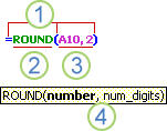
1. Structure. The structure of a function begins with an equal sign (=), followed by the function name, an opening parenthesis, the arguments for the function separated by commas, and a closing parenthesis.
2. Function name. For a list of available functions, click a cell and press SHIFT+F3.
3. Arguments. Arguments can be numbers, text, logical values such as TRUE or FALSE, arrays, error values such as #N/A, or cell references. The argument you designate must produce a valid value for that argument. Arguments can also be constants, formulas, or other functions.
4. Argument tooltip. A tooltip with the syntax and arguments appears as you type the function. For example, type =ROUND( and the tooltip appears. Tooltips appear only for built-in functions.
Entering functions
When you create a formula that contains a function, you can use the Insert Function dialog box to help you enter worksheet functions. As you enter a function into the formula, the Insert Function dialog box displays the name of the function, each of its arguments, a description of the function and each argument, the current result of the function, and the current result of the entire formula.
To make it easier to create and edit formulas and minimize typing and syntax errors, use Formula AutoComplete. After you type an = (equal sign) and beginning letters or a display trigger, Excel for the web displays, below the cell, a dynamic drop-down list of valid functions, arguments, and names that match the letters or trigger. You can then insert an item from the drop-down list into the formula.
Nesting functions
In certain cases, you may need to use a function as one of the arguments of another function. For example, the following formula uses a nested AVERAGE function and compares the result with the value 50.
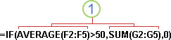
1. The AVERAGE and SUM functions are nested within the IF function.
Valid returns When a nested function is used as an argument, the nested function must return the same type of value that the argument uses. For example, if the argument returns a TRUE or FALSE value, the nested function must return a TRUE or FALSE value. If the function doesn’t, Excel for the web displays a #VALUE! error value.
Nesting level limits A formula can contain up to seven levels of nested functions. When one function (we’ll call this Function B) is used as an argument in another function (we’ll call this Function A), Function B acts as a second-level function. For example, the AVERAGE function and the SUM function are both second-level functions if they are used as arguments of the IF function. A function nested within the nested AVERAGE function is then a third-level function, and so on.
Using references in formulas
A reference identifies a cell or a range of cells on a worksheet, and tells Excel for the web where to look for the values or data you want to use in a formula. You can use references to use data contained in different parts of a worksheet in one formula or use the value from one cell in several formulas. You can also refer to cells on other sheets in the same workbook, and to other workbooks. References to cells in other workbooks are called links or external references.
The A1 reference style
The default reference style By default, Excel for the web uses the A1 reference style, which refers to columns with letters (A through XFD, for a total of 16,384 columns) and refers to rows with numbers (1 through 1,048,576). These letters and numbers are called row and column headings. To refer to a cell, enter the column letter followed by the row number. For example, B2 refers to the cell at the intersection of column B and row 2.
|
To refer to |
Use |
|
The cell in column A and row 10 |
A10 |
|
The range of cells in column A and rows 10 through 20 |
A10:A20 |
|
The range of cells in row 15 and columns B through E |
B15:E15 |
|
All cells in row 5 |
5:5 |
|
All cells in rows 5 through 10 |
5:10 |
|
All cells in column H |
H:H |
|
All cells in columns H through J |
H:J |
|
The range of cells in columns A through E and rows 10 through 20 |
A10:E20 |
Making a reference to another worksheet In the following example, the AVERAGE worksheet function calculates the average value for the range B1:B10 on the worksheet named Marketing in the same workbook.

1. Refers to the worksheet named Marketing
2. Refers to the range of cells between B1 and B10, inclusively
3. Separates the worksheet reference from the cell range reference
The difference between absolute, relative and mixed references
Relative references A relative cell reference in a formula, such as A1, is based on the relative position of the cell that contains the formula and the cell the reference refers to. If the position of the cell that contains the formula changes, the reference is changed. If you copy or fill the formula across rows or down columns, the reference automatically adjusts. By default, new formulas use relative references. For example, if you copy or fill a relative reference in cell B2 to cell B3, it automatically adjusts from =A1 to =A2.

Absolute references An absolute cell reference in a formula, such as $A$1, always refer to a cell in a specific location. If the position of the cell that contains the formula changes, the absolute reference remains the same. If you copy or fill the formula across rows or down columns, the absolute reference does not adjust. By default, new formulas use relative references, so you may need to switch them to absolute references. For example, if you copy or fill an absolute reference in cell B2 to cell B3, it stays the same in both cells: =$A$1.

Mixed references A mixed reference has either an absolute column and relative row, or absolute row and relative column. An absolute column reference takes the form $A1, $B1, and so on. An absolute row reference takes the form A$1, B$1, and so on. If the position of the cell that contains the formula changes, the relative reference is changed, and the absolute reference does not change. If you copy or fill the formula across rows or down columns, the relative reference automatically adjusts, and the absolute reference does not adjust. For example, if you copy or fill a mixed reference from cell A2 to B3, it adjusts from =A$1 to =B$1.

The 3-D reference style
Conveniently referencing multiple worksheets If you want to analyze data in the same cell or range of cells on multiple worksheets within a workbook, use a 3-D reference. A 3-D reference includes the cell or range reference, preceded by a range of worksheet names. Excel for the web uses any worksheets stored between the starting and ending names of the reference. For example, =SUM(Sheet2:Sheet13!B5) adds all the values contained in cell B5 on all the worksheets between and including Sheet 2 and Sheet 13.
-
You can use 3-D references to refer to cells on other sheets, to define names, and to create formulas by using the following functions: SUM, AVERAGE, AVERAGEA, COUNT, COUNTA, MAX, MAXA, MIN, MINA, PRODUCT, STDEV.P, STDEV.S, STDEVA, STDEVPA, VAR.P, VAR.S, VARA, and VARPA.
-
3-D references cannot be used in array formulas.
-
3-D references cannot be used with the intersection operator (a single space) or in formulas that use implicit intersection.
What occurs when you move, copy, insert, or delete worksheets The following examples explain what happens when you move, copy, insert, or delete worksheets that are included in a 3-D reference. The examples use the formula =SUM(Sheet2:Sheet6!A2:A5) to add cells A2 through A5 on worksheets 2 through 6.
-
Insert or copy If you insert or copy sheets between Sheet2 and Sheet6 (the endpoints in this example), Excel for the web includes all values in cells A2 through A5 from the added sheets in the calculations.
-
Delete If you delete sheets between Sheet2 and Sheet6, Excel for the web removes their values from the calculation.
-
Move If you move sheets from between Sheet2 and Sheet6 to a location outside the referenced sheet range, Excel for the web removes their values from the calculation.
-
Move an endpoint If you move Sheet2 or Sheet6 to another location in the same workbook, Excel for the web adjusts the calculation to accommodate the new range of sheets between them.
-
Delete an endpoint If you delete Sheet2 or Sheet6, Excel for the web adjusts the calculation to accommodate the range of sheets between them.
The R1C1 reference style
You can also use a reference style where both the rows and the columns on the worksheet are numbered. The R1C1 reference style is useful for computing row and column positions in macros. In the R1C1 style, Excel for the web indicates the location of a cell with an «R» followed by a row number and a «C» followed by a column number.
|
Reference |
Meaning |
|
R[-2]C |
A relative reference to the cell two rows up and in the same column |
|
R[2]C[2] |
A relative reference to the cell two rows down and two columns to the right |
|
R2C2 |
An absolute reference to the cell in the second row and in the second column |
|
R[-1] |
A relative reference to the entire row above the active cell |
|
R |
An absolute reference to the current row |
When you record a macro, Excel for the web records some commands by using the R1C1 reference style. For example, if you record a command, such as clicking the AutoSum button to insert a formula that adds a range of cells, Excel for the web records the formula by using R1C1 style, not A1 style, references.
Using names in formulas
You can create defined names to represent cells, ranges of cells, formulas, constants, or Excel for the web tables. A name is a meaningful shorthand that makes it easier to understand the purpose of a cell reference, constant, formula, or table, each of which may be difficult to comprehend at first glance. The following information shows common examples of names and how using them in formulas can improve clarity and make formulas easier to understand.
|
Example Type |
Example, using ranges instead of names |
Example, using names |
|
Reference |
=SUM(A16:A20) |
=SUM(Sales) |
|
Constant |
=PRODUCT(A12,9.5%) |
=PRODUCT(Price,KCTaxRate) |
|
Formula |
=TEXT(VLOOKUP(MAX(A16,A20),A16:B20,2,FALSE),»m/dd/yyyy») |
=TEXT(VLOOKUP(MAX(Sales),SalesInfo,2,FALSE),»m/dd/yyyy») |
|
Table |
A22:B25 |
=PRODUCT(Price,Table1[@Tax Rate]) |
Types of names
There are several types of names that you can create and use.
Defined name A name that represents a cell, range of cells, formula, or constant value. You can create your own defined name. Also, Excel for the web sometimes creates a defined name for you, such as when you set a print area.
Table name A name for an Excel for the web table, which is a collection of data about a particular subject that is stored in records (rows) and fields (columns). Excel for the web creates a default Excel for the web table name of «Table1», «Table2», and so on, each time you insert an Excel for the web table, but you can change these names to make them more meaningful.
Creating and entering names
You create a name by using Create a name from selection. You can conveniently create names from existing row and column labels by using a selection of cells in the worksheet.
Note: By default, names use absolute cell references.
You can enter a name by:
-
Typing Typing the name, for example, as an argument to a formula.
-
Using Formula AutoComplete Use the Formula AutoComplete drop-down list, where valid names are automatically listed for you.
Using array formulas and array constants
Excel for the web doesn’t support creating array formulas. You can view the results of array formulas created in Excel desktop application, but you can’t edit or recalculate them. If you have the Excel desktop application, click Open in Excel to work with arrays.
The following array example calculates the total value of an array of stock prices and shares, without using a row of cells to calculate and display the individual values for each stock.
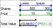
When you enter the formula ={SUM(B2:D2*B3:D3)} as an array formula, it multiples the Shares and Price for each stock, and then adds the results of those calculations together.
To calculate multiple results Some worksheet functions return arrays of values, or require an array of values as an argument. To calculate multiple results with an array formula, you must enter the array into a range of cells that has the same number of rows and columns as the array arguments.
For example, given a series of three sales figures (in column B) for a series of three months (in column A), the TREND function determines the straight-line values for the sales figures. To display all the results of the formula, it is entered into three cells in column C (C1:C3).
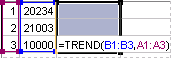
When you enter the formula =TREND(B1:B3,A1:A3) as an array formula, it produces three separate results (22196, 17079, and 11962), based on the three sales figures and the three months.
Using array constants
In an ordinary formula, you can enter a reference to a cell containing a value, or the value itself, also called a constant. Similarly, in an array formula you can enter a reference to an array, or enter the array of values contained within the cells, also called an array constant. Array formulas accept constants in the same way that non-array formulas do, but you must enter the array constants in a certain format.
Array constants can contain numbers, text, logical values such as TRUE or FALSE, or error values such as #N/A. Different types of values can be in the same array constant — for example, {1,3,4;TRUE,FALSE,TRUE}. Numbers in array constants can be in integer, decimal, or scientific format. Text must be enclosed in double quotation marks — for example, «Tuesday».
Array constants cannot contain cell references, columns or rows of unequal length, formulas, or the special characters $ (dollar sign), parentheses, or % (percent sign).
When you format array constants, make sure you:
-
Enclose them in braces ( { } ).
-
Separate values in different columns by using commas (,). For example, to represent the values 10, 20, 30, and 40, you enter {10,20,30,40}. This array constant is known as a 1-by-4 array and is equivalent to a 1-row-by-4-column reference.
-
Separate values in different rows by using semicolons (;). For example, to represent the values 10, 20, 30, and 40 in one row and 50, 60, 70, and 80 in the row immediately below, you enter a 2-by-4 array constant: {10,20,30,40;50,60,70,80}.
Excel Calculations (Table of Contents)
- Introduction to Excel Calculations
- How to Calculate Basic Functions in Excel?
Introduction to Excel Calculations
Excel is used for a variety of functions, but the basic area why excel was introduced was for handling calculations of day to day work. Like adding, subtracting, multiplication, etc., numbers are used for different purposes for a different domains. Though there are other tools for basic calculations but standoff of using excel is its flexibility and the perception for the viewer it gives; for instance, we can add two numbers in the calculator as well, but the numbers mentioned in the excel sheet can be entered in two cells and used for other functions as well subtraction, division, etc.
Let’s have a quick look at some of the calculations to get a better understanding.
How to Calculate Basic Functions in Excel?
Let us start with the basic calculations and gradually will move further.
You can download this Excel Calculations Template here – Excel Calculations Template
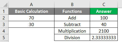
List of calculations that one already knows.
After using the above formula output shown below.
Similarly, a formula is used in Cell C3, C4, C5.
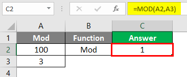
#1 – MOD
Use to get the remainder of two numbers when divided.
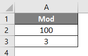
Apply the MOD formula in cell C2.
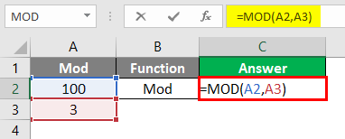
After using the MOD, the Formula output is shown below.
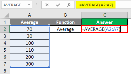
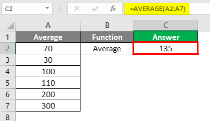
#2 – Average
Use to take the median or average between the range of numbers.
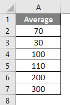
Apply the Average formula in cell C2.
After using the AVERAGE Formula output shown below.
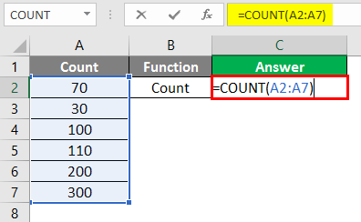
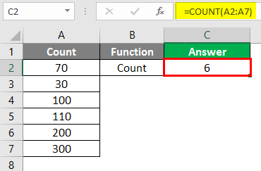
#3 – Count
Use to count a number of cells in data.
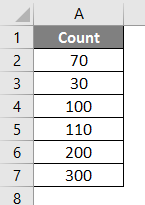
Apply the COUNT formula in Cell C2.
After using the COUNT Formula output shown below.
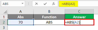
#4 – Abs
Use for removing the sign from the number
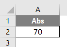
Apply the ABS formula in Cell C2.
After using the ABS Formula output shown below.
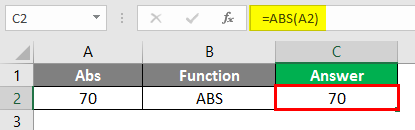
Note: Abs function can only be used for one cell at a time.
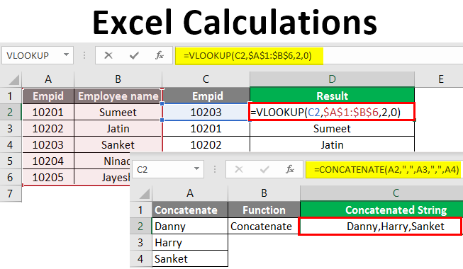
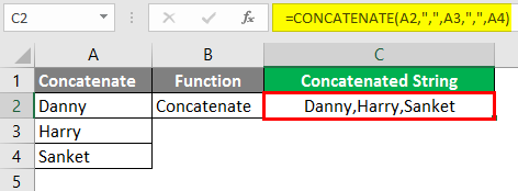
#5 – Concatenate
Use for merging text from two or more cells.
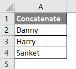
Apply the Concatenate formula in Cell C2.
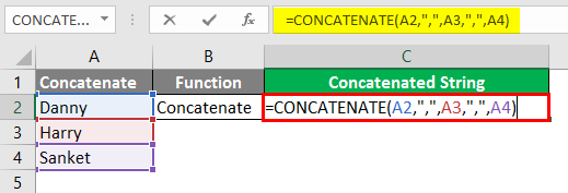
After using the CONCATENATE Formula output as shown below.
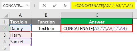
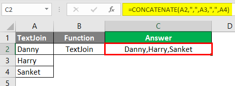
#6 – Text Join
Use for merging text from two or more cells if one has a range; this formula is recommended, though this is a new formula and may not be available in previous versions.
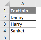
Apply the Concatenate formula in Cell C2.
After using the CONCATENATE Formula, the output is shown below.
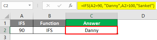
#7 – IFS
Use instead of IF condition when there are too many conditions to be given, i.e. nested if-else.
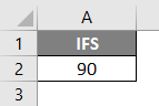
Apply the IFS formula in Cell C2.
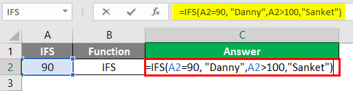
After using the IFS, the Formula output is shown below.
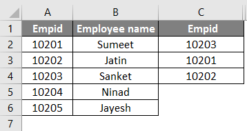
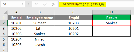
#8 – VLOOKUP
VLOOKUP function is used in various situations, such as comparing data with one column and validating whether the data is present in the current column. Retrieving the data of the dependent column by comparing the data of the current column with the column on which the dependent column depends on; for this, below is the example for one’s preference.
Explanation: The “Third column Empid” data is first compared with Empid, and with respect to the “Empid”, the name is retrieved in the “Result” column. For Example, 10203 from the “Third column Empid” is compared with the “Empid” column i.e.with 10203 and the corresponding name Sanket is retrieved in the “Result” column.
Apply the VLOOKUP formula in cell C2.
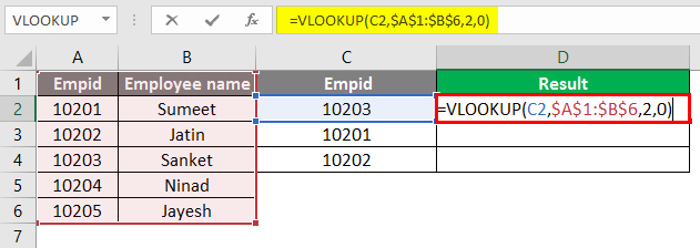
After using the VLOOKUP Formula, the output is shown below.
After using the VLOOKUP Formula, the output is shown below.
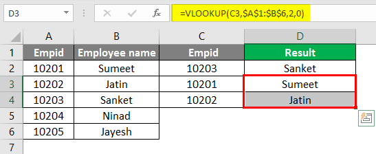
Note: Lookup can be used for different applications, like checking whether the third column is present in the Empid column.
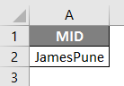
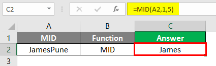
#9 – MID
Use for splitting the text or, in easy terms, can be used as a substring.
Apply the MID formula in Cell C2.
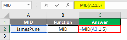
After using the MID Formula output shown below.
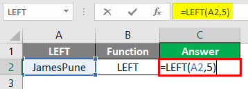
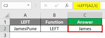
#10 – LEFT
Use the LEFT function when you want to extract characters starting at the left side of the text.
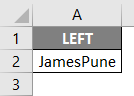
Apply the LEFT formula in cell C2.
After using the LEFT, the Formula output is shown below.
#11 – RIGHT
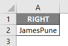
Use the RIGHT function when you want to extract characters starting at the right side of the text.
Apply the RIGHT formula in Cell C2.
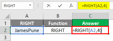
After using the RIGHT Formula, the output is shown below.
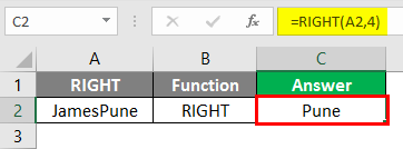
Explanation: In the above example, from the text value JamesPune, we only need James, so we use the MID function to split the JamesPune to James as shown in the formulae column. The same goes with a LEFT function where one can use it to split the string from the left side and the RIGHT function to split the string from the right side, as shown in the formulae.
Note: MID, LEFT, and RIGHT functions can also be used with a combination such as with the Find function, etc.
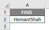
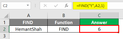
#12 – FIND
Use for searching the character’s position in the string.
Apply the FIND formula in cell C2.
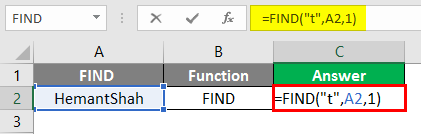
After using the FIND, the Formula output is shown below.
#13 – LEN
Use for checking the length of the string.
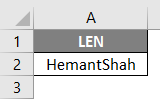
Apply the LEN formula in cell C2.
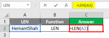
After using the LEN, the Formula output is shown below.
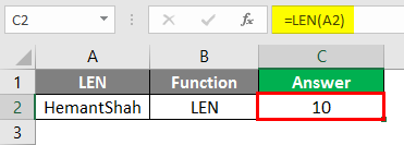
Explanation: The FIND function is used for searching the character’s position in the string, like the letter “t” position in the above text is at 6 positions. LEN in the above example gives the length of the string
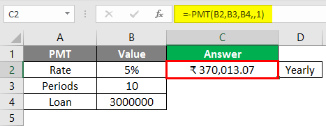
#14 – PMT
It is used for the calculation of monthly installments one has to pay.
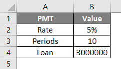
Apply the PMT formula in cell C2.
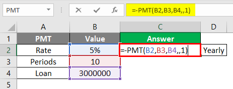
After using the PMT, the Formula output is shown below.
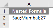
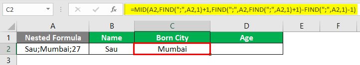
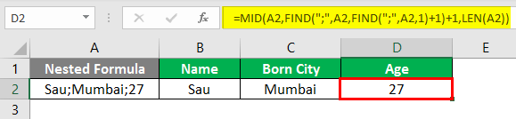
#15 – Nested Formula
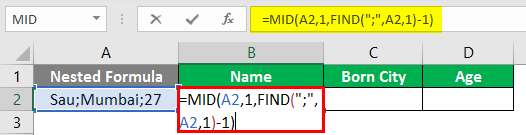
Used when our conditions have two to three functions to be used. Suppose we have a text Sau; Mumbai;27 and we want to separate as the Name then we would go following formula as =MID(A2,1, FIND(“;”, A2,1)-1).
Apply the MID formula in cell C2.
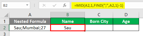
After using the above Formula output shown below.
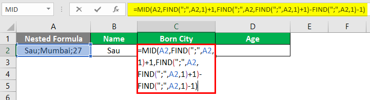
After using the above Formula, the output is shown below.
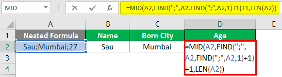
After using the above Formula, the output is shown below.
Explanation:
So here for Name, we only want “Sau”, so here we use the combination of MID function, which will help us to split the string, and the FIND function helps to locate the position of; in the string, i.e.as per MID function it needs:
MID(Text_value,start_position, end_position)
Text_value: Sau;Mumbai;27
Start_position: 1
End_position: Position of the first semicolon by FIND function
FIND (find_text, within_text, [start_num])
Find_text = ;
Within_text= Sau;Mumbai;27
Start_num=1
So here, the FIND function gives the position as 4; hence, the MID function looks like this MID(A98,1,4-1). MID(A98,1,3), which would result in “Sau” as shown in below fig:
Pros
- The excel calculations provide a robust function.
- Calculations can be dynamic.
- Nested Functions are possible.
- More functions are getting added up, helping users ease and avoid more Nested Formulae Example: PMT formula.
Cons
- Nested Formulae becomes complex to apply.
- Sometimes maintenance and usage of the formulae become difficult if the user is not prone to excel.
Things to Remember About Excel Calculations
- Save your worksheet after every application of excel calculations
- Functions of excel are getting added up day by day, so it’s good to stay updated and to avoid usage of Nested Formulae
- Whenever one applies the function in excel, one can click on the Tab button to autocomplete the function name, i.e. if one wants to enter Sum function in a cell, then choose the cell and write “ = S” and press Tab, the function would get autocompleted and, one can also see the value which the function ask for
Recommended Articles
This is a guide to Excel Calculations. Here we discuss How to Calculate Basic Functions in Excel along with practical examples and a downloadable excel template. You can also go through our other suggested articles –
- Count Names in Excel
- NPV Formula in Excel
- Mixed Reference in Excel
- VBA Right | Excel Template
Contents
- Tools, Calculators and Simulations
- Dashboards and Reports with Charts
- Automate Jobs with VBA macros
- Solver Add-in & Statistical Analysis
- Data Entry and Lists
- Games in Excel!
- Educational use with Interactive features
- Create Cheatsheets with Excel
- Diagrams, Mockups, Gantt Charts
- Fetch live data from web
- Excel as a Database
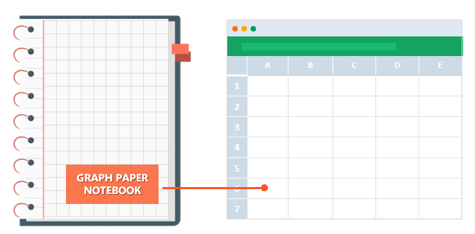
Excel is one of the most used software in today’s digital world. Most people quickly open up an Excel file when they need to write or calculate anything. It is like “paper”. (remember those graph notebooks from school times..)
Actually, this is not only specific to Microsoft’s Excel but most of the spreadsheet software like open office or google sheets. However, we will focus on Excel and what can you do with it today, as it offers huge flexibility you will discover below.
Let’s start with the main usage areas of Excel. As we all know, spreadsheets are designed to make calculations easier. So they contain “formulas”. They allow us to make basic math like summing, multiplying, finding average as well as advanced calculations like regression analysis, conversions, and so on.
When we combine these powerful math features with some tables, lists, or other UI elements, we can come up with a calculator. And most of the time they will be dynamic (meaning that when you change a parameter all the rest of the calculations will adapt accordingly)
Below see an example from our past studies as Someka:
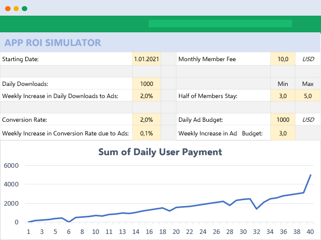
We have built this calculator for an app development company executive. He was changing the parameters he wants and sees the outcomes immediately.
This is great especially when you try to make big “models” in excel. Financial Modeling is one of the most used application areas of these big models. If we tried to do this with pen-paper (which used to be the way once upon a time) it would be horrible I guess:

Financial modeling is also being used to test the excel skills of experts. They even make a competition for it: ModelOff
We also have a tool for startups to make a feasibility study playing with their own variables:
This is a comprehensive Feasibility Study Excel Template for app startups with download projections, costs, financial calculations, charts, dashboard, and more.
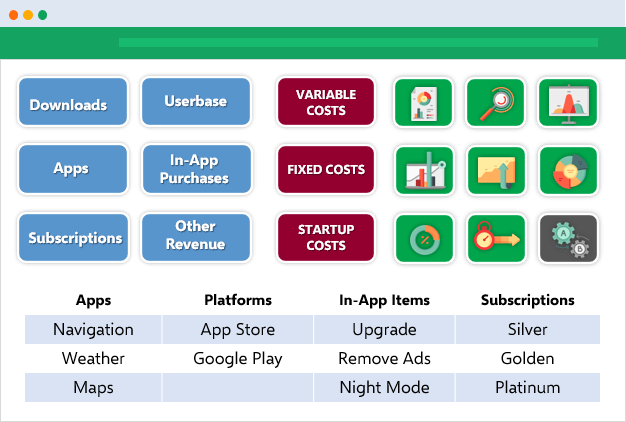
The business world is demanding. It is not enough just to make the calculations, set up your tables, and write the text. You have to create pie charts, trends, line graphs, and many more. Whether you are getting prepared for your pitch or make a presentation in your company, you can use Excel’s chart features.
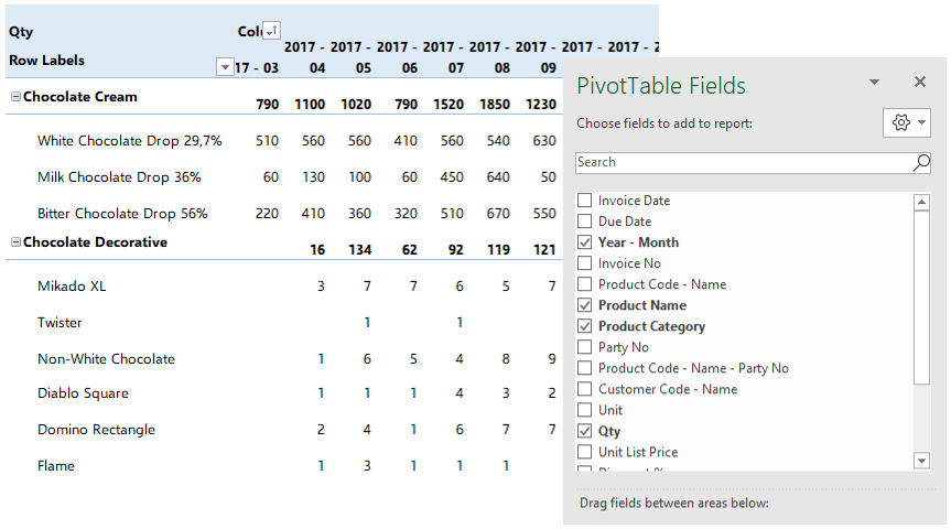
Pivot Tables
One of the greatest features which Excel offers is Pivot tables. This is an advanced Excel tool that helps you create dynamic summary reports from raw data very easily. After you create your table you can play with parameters easily with a drag and drop interface.
It looks like this:
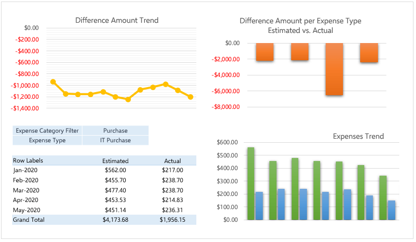
Dashboards
Complex excel models do have lots of variables, calculations, and settings. And instead of managing all variables one by one on different sheets, different places it is a very good idea to put them together like a “control panel”.
You can think dashboards as cockpits of planes.
Recently dashboards became very popular. There are lots of training videos about how to build and design control panels for our excel models. Actually, they are not so different from the rest of the calculations.
But the main idea is: if there is something you may want to change, later on, don’t write it directly in the formula but bind it to a variable.
Let’s say you are building a sales report for your manager. He asks you to make the file changeable so that he can see the results in US dollars or Euros according to the situation. Instead of writing an Fx rate into the calculations, you should bind this to a cell that you can play with later on.
Like this:
This may seem so obvious to some of you. But this is the basic approach of all dashboards in excel files. Of course, you can improve it with more complex formulas, buttons, cool charts, and even VBA but the main idea stands still.
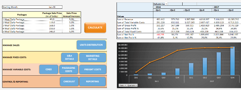
Here is an example of a complete set of the dashboard:
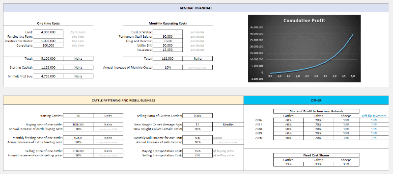
Or a dashboard for a livestock feasibility study:
If you are interested in Sales Dashboards, you may want to check out our Excel template:
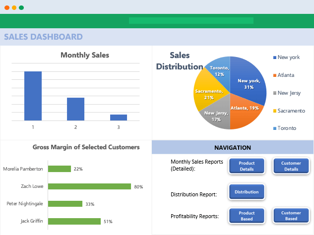
This is an interactive Sales Report Template in Excel. Features a dashboard with profitability, sales analysis and charts.
Other than that, Marketing ROI Calculator would be very helpful to prioritize your marketing campaigns in Excel:
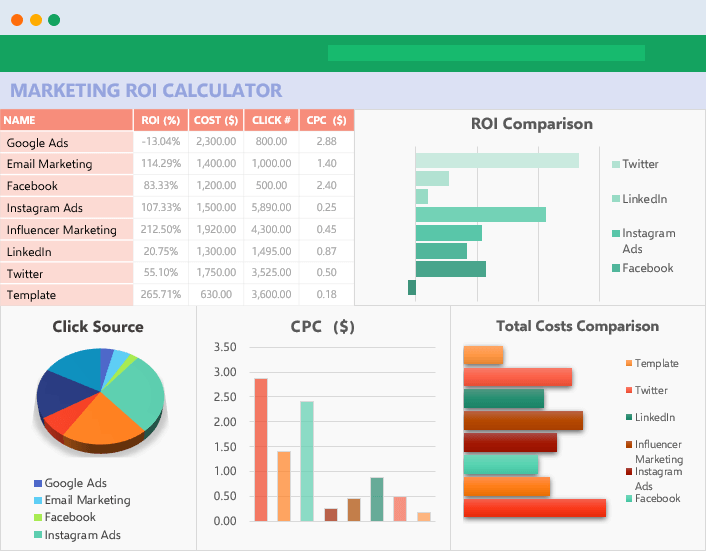
It will provide essential metrics and help you to manage all your marketing campaign channels in one place.
Most of the users who use Excel extensively are already coding. But if you ask them whether they know how to code most probably they will say no. Of course, writing formulas is a very small part of the things you can do with VBA. It is a strong programming language that lets you create small scripts (macros), user forms, user-defined functions, add-ins, and even games! (which we will touch below separately)
I will not dive into VBA here since it is a detailed area. But there are some basic things that will be beneficial to know for those who use Excel often:
- You can record macros for repeating jobs: You don’t need to code from scratch. Just click on the record macro button and it will write the code for you in the background. (If you want, you can modify later on)
- It extends the borders of Excel world. If you feel like you are limited somehow in Excel, you are more like an advanced user. It is time to get a little bit into VBA.
- You can create user forms with VBA only. If you see something like this, know that it is using VBA:
VBA is quite powerful and if you work with Excel extensively you won’t regret learning a bit. For example wouldn’t it be nice if you could send bulk emails from an Excel spreadsheat with a button click?
It is not surprising for spreadsheet software like Excel to offer advanced math techniques to make more complicated studies. (To be honest, I am not a statistics expert but with an engineering background, I will try to do my best to explain the basics. Feel free to correct me if I’m wrong)
Data analysis is a trending concept for recent years with the development of powerful computers and improved software. We are collecting and recording much much more data compared to the past. Take a look at this chart to understand what I mean:

Especially this part:
“more data has been created in the past two years than in the entire previous history of the human race”
It is a bit frightening, isn’t it? Ok, we are not going to dive into the “Big Data” world. Let’s get back to our humble excel world.
As we collect this much data, some people will want to analyze it. Otherwise, it makes no sense to spend billions of dollars on those data centers. Excel has built-in functions for basic descriptive statistics methods like Mean, Median, Mode, Standard Deviation, Variance etc.
But if we want to go a bit further I will mention two Excel features (actually add-ins) at this step: Solver and Regression Analysis
Solver
Have you ever heard of “optimization”? When we have more than one parameters that affect the outcome, we can only have a most optimized solution rather than a maximum solution. This may sound weird but it is very valid in our daily lives.
One of the simplest and popular examples is: Farmer Fence Optimization Problem
“A farmer owns 500 meters of the fence and wants to enclose the largest possible rectangular area. How should he use his fence?”
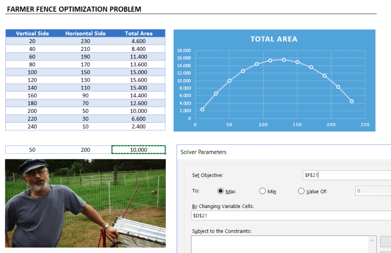
This is a very simple example to explain what a solver does. But actually, you can run much more complicated data sets with Solver.
Regression Analysis
Since this is a bit advanced topic for this blog post, I will only touch the surface.
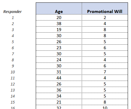
In most simple terms, regression analysis helps you find the correlation between the variables. For example, you may want to know what is the relation between the number of birds flown over your head and the money you earned today. (sorry for the silly example. No, I am not curious about it  You will need to gather sample data and put in an analysis to see if there is any correlation.
It seems something like this:
You put your data:
Run the regression from Analysis Toolpak:
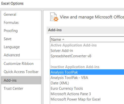
And get results something like this:
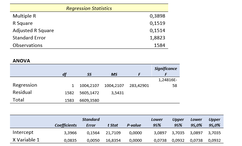
Of course, there is much more sophisticated software to run data analysis. However, there is a joke in business intelligence communities:
- What is the most used feature of any business intelligence solution?
- It is “Export to Excel”
Looks like we won’t stop using Excel anytime soon.
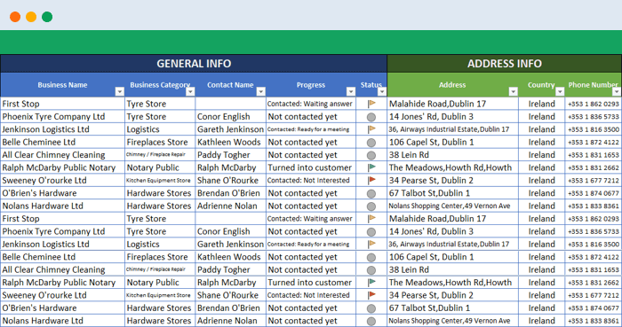
Coming back from boring data analysis world, let’s mention the simplest and most handy usage area of excel: Make Lists!
It is already self-explaining so I won’t bother with the details. When you want to list down some simple data, take notes, create to-do lists, or anything. Just open the excel and write it down. Did we mention that “paper alternative” thing? Oh yes, we did.
A lead list example:
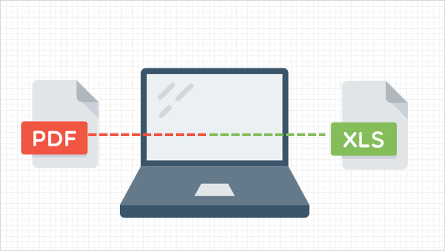
You can also convert PDF files into Excel files in order to make it easier to work on. This can be done automatically with some software. But some pdf files cannot be processed automatically (like handwritten documents, scanned invoices, etc). You will need to do it manually.
When you want to play with the data on a web page, you can easily copy-paste it into an excel file and then you can sort, filter or do anything you want:
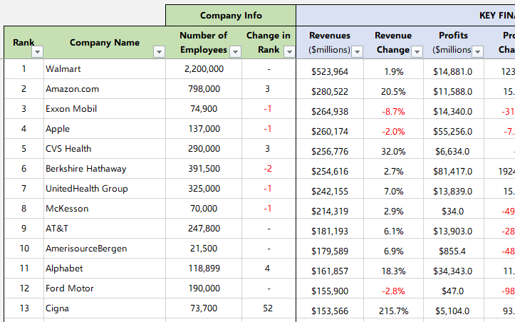
For example, Fortune 500 US List:
Everybody loves to-do lists. And we have created useful to-do list in Excel for business or personal uses. Check it out, it is free:
To-Do List Excel Template
We already mentioned this in the VBA section above. But it is worth to talk a bit more.
Visual Basic allows you to code complex things like games as well. But of course, don’t expect a GTA or FIFA. Things like chess, sudoku, or Monopoly is OK. But, a few people have gone far and created more complicated things, like an RPG game. Take a look at this:
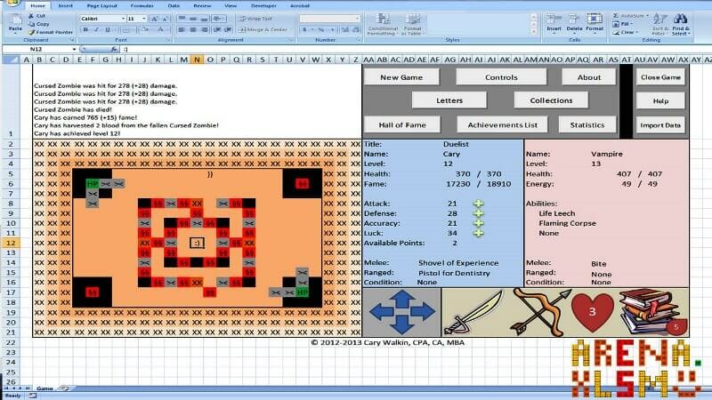
This game has been created by an accountant, Cary Walkin. I know it doesn’t look great but it is in Excel! (you can play it at the office  )
)
Another example:

A flight simulator in Excel?? Is it the same thing we use to sum up the sales figures? Lol yeah.
You can also embed flash games into Excel (like Super Mario, Angry Birds or whatever) But I count them off as they are not built with VBA.
As we mentioned in the Financial Modeling section, Excel is quite good for creating dynamic results according to the inputs. We get the benefit of this to create interactive tools.
One example that comes to my mind is this spreadsheet, guys from San Francisco have prepared:

I haven’t tried it myself but an Excel tutorial in Excel. Liked the idea!
Another similar interactive Excel learning tool is from Keyskillset:
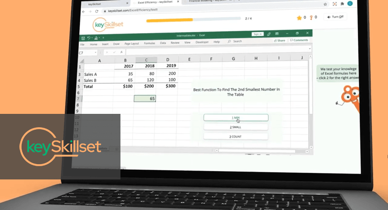
Actually, this is not completely in Excel and works as separate software but I liked how they combine the Excel training with gamification features.
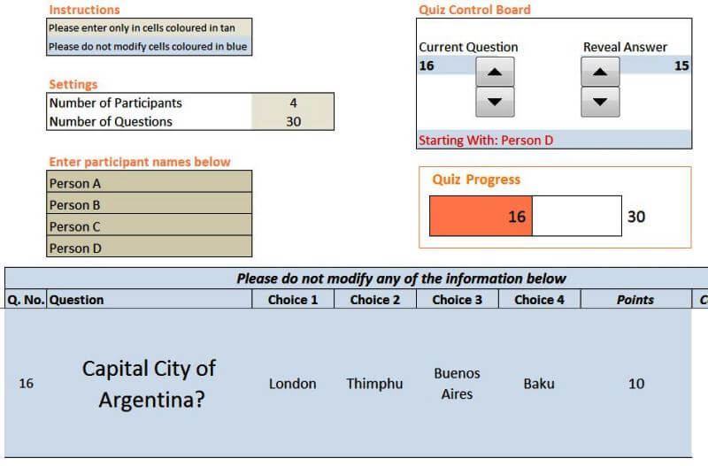
Quizzes are good tools for interactive learning and you can prepare in Excel as well. A quizmaster template from indzara.com:
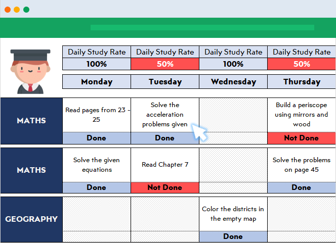
A student lesson plan template in excel which we have prepared recently:
You can learn Excel in Excel!
As said: Practice Makes Perfect!
You can test your Excel skills in Excel with Excel Formulas Trainer:
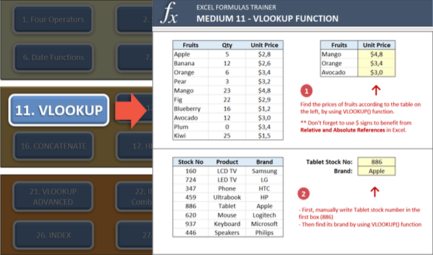
This is actually an Excel template prepared with VBA macros and basically works as a practice worksheet. It has 30 sections and around 100 questions. You can learn VLOOKUP, IF and much more excel formulas by doing. If you like the idea of “learning by doing”, then it is worth to check.
Also, this online course from GoSkills is for everyone as well, covering beginner, intermediate and advanced lessons.
By cheat sheets, we don’t refer to the piece of paper with information written down on it that an unethical person might create if they weren’t prepared for a test. What we mean is a reference tool that provides simple, brief instructions for accomplishing a specific task. We use this term because it is highly popular recently.
For example, this is a cheat sheet:
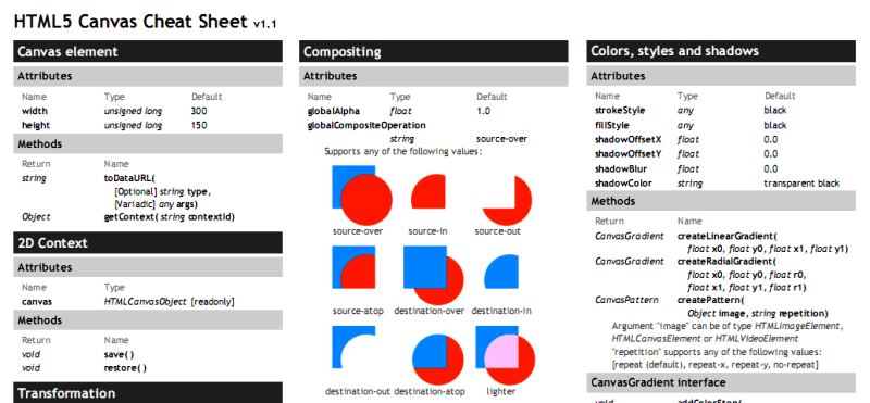
This compacted and summarized info is very useful in many aspects. When you try to memorize things, lookup, reference, etc. And can be easily created with Excel. Let’s make a Google search for a cheat sheet made in Excel.
This one is from Dave Child (cheatography.com) and I was also using this one I first learned HTML:
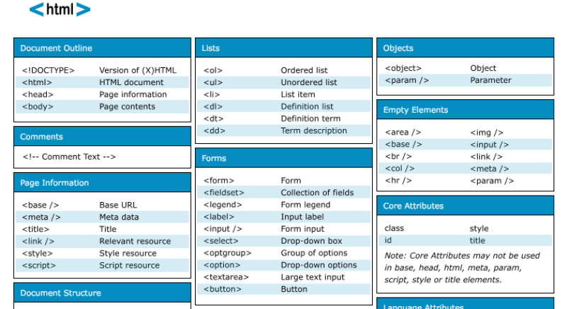
The last example is an Excel Cheatsheet made for Excel shortcuts:
Of course, if you are looking for stylish infographics and cheat sheets, you should check out design software.
I know Excel is maybe not the best tool to do these. There are great programs or websites to make mockups, diagrams, brainstorming, mind-mapping, or project scheduling. But there are habits as well. Even though I am very open to try and use these kinds of brand-new tools, I find myself using excel for a mockup or a mind map. (select shapes, put notes, put arrows, change colors etc. Omg it is tedious)
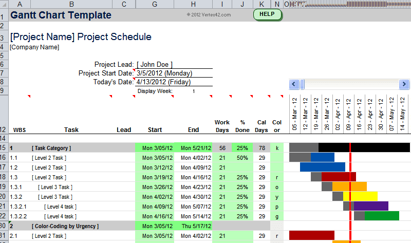
Gantt charts can be a bit old-school as agile project management methods are increasing in popularity, they are still being used widely. There are several Gantt chart excel templates on the web.
A Gantt chart example from vertex42.com:
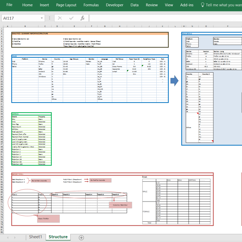
I just found out a reporting structure mockup I have prepared in Excel once upon a time:
By the way, did you see our Automatic Organization Chart Generator?
This is an Excel template that lets you create organization charts from Excel lists with a click of a button. It can be useful for small business owners and Human Resources departments.
These type of charts are directly related to Excel as most of the companies already keep their data in spreadsheets. But I also know people who even build their website mockups in Excel (with links to other sections, placement of buttons, sliders etc.).
Sometimes you may need your excel files to be updated automatically from a live data source. For example, if you are making a stock market analysis and want the latest data of some stock prices at NYSE, you can connect your Excel file to a data feed and let it take the latest info automatically (unless you want to input them one by one!)
As this is a comprehensive topic I will leave it for another post. But here is a few things you can fetch into excel:
- Stock prices
- Match results of soccer, NBA, NFL or any sports games (from live score sites)
- Fx rates
- Real-time flight data of airports
- Any info in a shared database (whether it is your company intranet or public)
This topic is getting more and more important as most data is kept on cloud systems. We don’t download info bits to our computers as we used to do in the past. So, Microsoft is working hard to improve the web integration of Excel.
Recommended Reading: Can Excel Extract Data From Website?
Yes, it is not the best idea to use Excel as a database. Because it is not designed for this purpose. Queries will take a long time especially when data gets bigger. It can be unreliable sometimes and not very secure. It is all accepted. However, we are not always after a complete set of the database systems and it can serve us as a mini-warehouse for our little data.

For example, if you keep records of your invoice data and want to make some sales analysis, it can be a good starting point. If later, you want to see more details, want to record more breakdowns you will need to move to a “real database”. It can be Access, SQL or anything. Just keep an eye on your Excel file because it has a maximum of 1 million rows.
Some of you may say “hey, it is more than enough, isn’t it?”
Generally yes. But you cannot believe how data increase in size when you want to see details. I remember when I was working as an analyst in a game development company, we were holding records of 1+ billion rows of data.
Precisely because of that, we have built some of our Excel templates (which is the favorite feature of all the users) with a database section. You may check our Invoice Generators and see how invoice recording would be super easy in Excel!
Conclusion
As the internet gets more available for everybody people started to use collaboration platforms more than before. In this aspect, online spreadsheet applications, like Google Sheets, increase in popularity and stands as a competitor to Microsoft’s Excel. Other free alternatives like open office or libre office are also popular. But if you need the advanced functionalities of Excel there is still no substitute.

Microsoft is improving the software actively. PowerPivot, Power BI, and Excel Online are all brand new features they developed recently. We will wait and see how things evolve in the following years. (investintech.com has made interviews with Excel experts about the future of Excel)
I tried to cover most of the things that can be done with Excel. If I have missed anything or if you find any errors, let me know by commenting down or sending an email.
Also, don’t forget to check our Excel Templates Collection. You may find something useful for yourself:
Excel Templates and Spreadsheets – Someka
Ready solutions for Excel with the help of formulas working with data spans in the process of complex computations and calculations.
Computing operations with the help of formulas
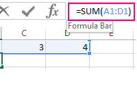 The Formula Bar in Excel, its settings and the purpose.
How to use the formula string and what advantages does it provide for entering and editing data in cells? How to enable or disable the formula bar in the program settings.
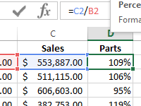 Percentage of the plan implementation by formula in Excel.
The examples of two formulas for calculating of percentages from numbers when analyzing the implementation of sales plans. The example, when and how to use the percentage format of cells.
Time-saving ways to insert formulas into Excel
Basic Excel Formulas Guide
Mastering the basic Excel formulas is critical for beginners to become highly proficient in financial analysis. Microsoft Excel is considered the industry standard piece of software in data analysis. Microsoft’s spreadsheet program also happens to be one of the most preferred software by investment bankers and financial analysts in data processing, financial modeling, and presentation.
This guide will provide an overview and list of some basic Excel functions.
Once you’ve mastered this list, move on to CFI’s advanced Excel formulas guide!
Basic Terms in Excel
There are two basic ways to perform calculations in Excel: Formulas and Functions.
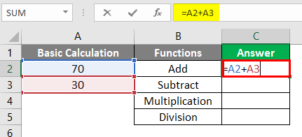
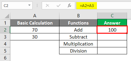
1. Formulas
In Excel, a formula is an expression that operates on values in a range of cells or a cell. For example, =A1+A2+A3, which finds the sum of the range of values from cell A1 to cell A3.
2. Functions
Functions are predefined formulas in Excel. They eliminate laborious manual entry of formulas while giving them human-friendly names. For example: =SUM(A1:A3). The function sums all the values from A1 to A3.
Key Highlights
- Excel is still the industry benchmark for financial analysis and modeling across almost all corporate finance functions. This course is designed to highlight some of the most important basic Excel formulas.
- Mastering these will help a learner build confidence in Excel and move on to more difficult functions and formulas.
- There are also several different ways to enter a function in Excel, as shown below.
Five Time-saving Ways to Insert Data into Excel
When analyzing data, there are five common ways of inserting basic Excel formulas. Each strategy comes with its own advantages. Therefore, before diving further into the main formulas, we’ll clarify those methods, so you can create your preferred workflow earlier on.
1. Simple insertion: Typing a formula inside the cell
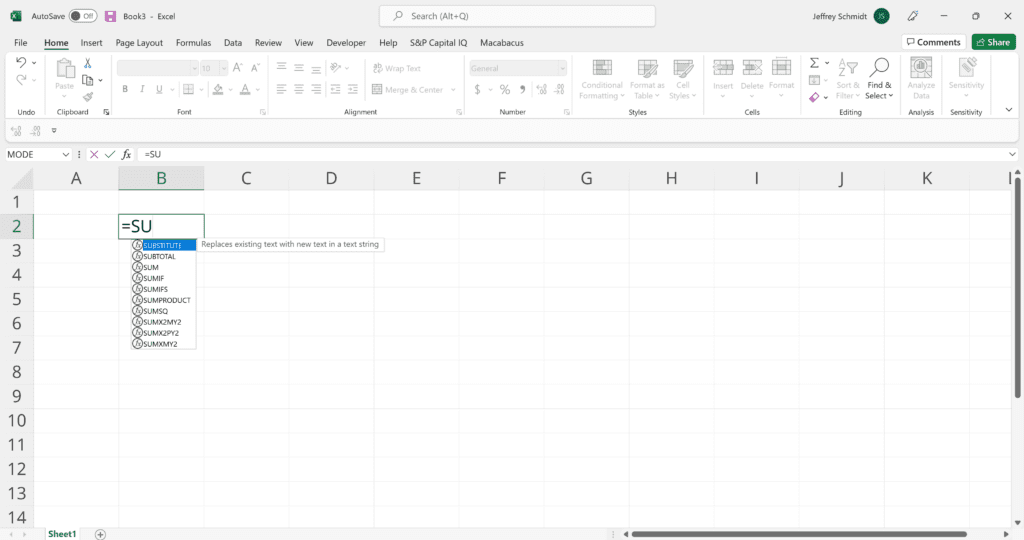
Typing a formula in a cell or the formula bar is the most straightforward method of inserting basic Excel formulas. The process usually starts by typing an equal sign, followed by the name of an Excel function.
Excel is quite intelligent in that when you start typing the name of the function, a pop-up function hint will show (see below). It’s from this list you’ll select your preference. However, don’t press the Enter key after making your selection. Instead, press the Tab key and Excel will automatically fill in the function name.
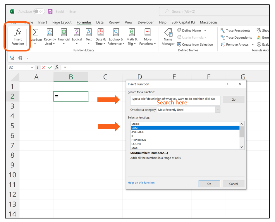
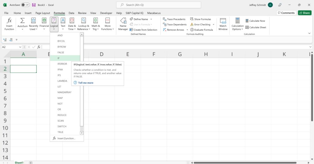
2. Using Insert Function Option from Formulas Tab
If you want full control of your function’s insertion, using the Excel Insert Function dialogue box is all you ever need. To achieve this, go to the Formulas tab and select the first menu labeled Insert Function. The dialogue box will contain all the functions you need to complete your financial analysis.
3. Selecting a Formula from One of the Groups in Formula Tab
This option is for those who want to delve into their favorite functions quickly. To find this menu, navigate to the Formulas tab and select your preferred group. Click to show a sub-menu filled with a list of functions.
From there, you can select your preference. However, if you find your preferred group is not on the tab, click on the More Functions option – it’s probably just hidden there.
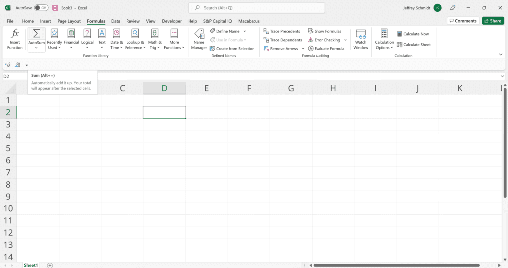
4. Using AutoSum Option
For quick and everyday tasks, the AutoSum function is your go-to option. Navigate to the Formulas tab and click the AutoSum option. Then click the caret to show other hidden formulas. This option is also available in the Home tab.
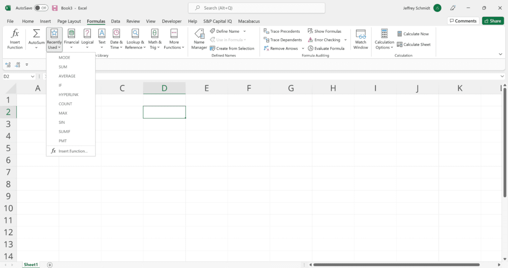
5. Quick Insert: Use Recently Used Tabs
If you find re-typing your most recent formula a monotonous task, then use the Recently Used selection. It’s on the Formulas tab, a third menu option just next to AutoSum.
Free Excel Formulas YouTube Tutorial
Watch CFI’s FREE video tutorial to quickly learn the most important Excel formulas. By watching the video demonstration you’ll quickly learn the most important formulas and functions.
Seven Basic Excel Formulas For Your Workflow
Since you’re now able to insert your preferred formulas and function correctly, let’s check some fundamental Excel functions to get you started.
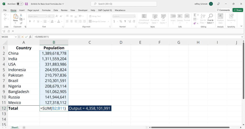
1. SUM
The SUM function is the first must-know formula in Excel. It usually aggregates values from a selection of columns or rows from your selected range.
=SUM(number1, [number2], …)
Example:
=SUM(B2:G2) – A simple selection that sums the values of a row.
=SUM(A2:A8) – A simple selection that sums the values of a column.
=SUM(A2:A7, A9, A12:A15) – A sophisticated collection that sums values from range A2 to A7, skips A8, adds A9, jumps A10 and A11, then finally adds from A12 to A15.
=SUM(A2:A8)/20 – Shows you can also turn your function into a formula.
2. AVERAGE
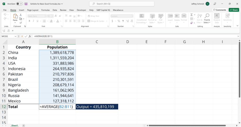
The AVERAGE function should remind you of simple averages of data, such as the average number of shareholders in a given shareholding pool.
=AVERAGE(number1, [number2], …)
Example:
=AVERAGE(B2:B11) – Shows a simple average, also similar to (SUM(B2:B11)/10)
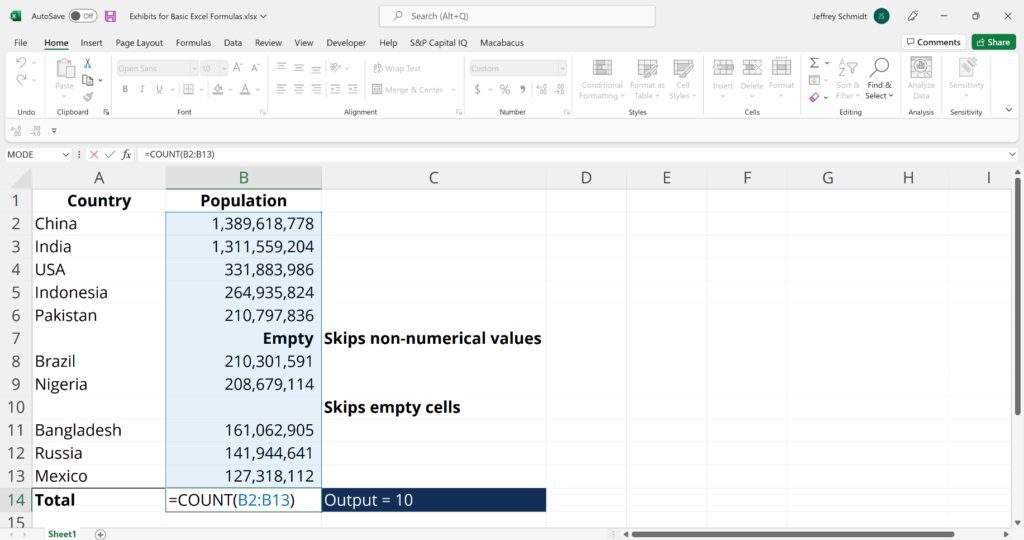
3. COUNT
The COUNT function counts all cells in a given range that contain only numeric values.
=COUNT(value1, [value2], …)
Example:
COUNT(A:A) – Counts all values that are numerical in A column. However, you must adjust the range inside the formula to count rows.
COUNT(A1:C1) – Now it can count rows.
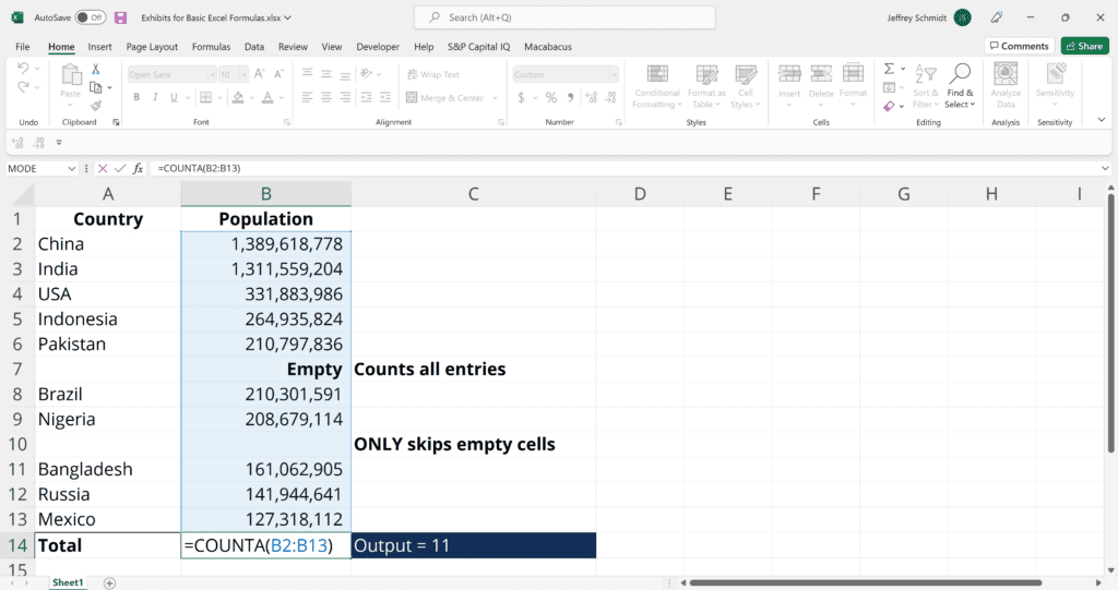
4. COUNTA
Like the COUNT function, COUNTA counts all cells in a given rage. However, it counts all cells regardless of type. That is, unlike COUNT that only counts numerics, it also counts dates, times, strings, logical values, errors, empty string, or text.
=COUNTA(value1, [value2], …)
Example:
COUNTA(C2:C13) – Counts rows 2 to 13 in column C regardless of type. However, like COUNT, you can’t use the same formula to count rows. You must make an adjustment to the selection inside the brackets – for example, COUNTA(C2:H2) will count columns C to H
5. IF
The IF function is often used when you want to sort your data according to a given logic. The best part of the IF formula is that you can embed formulas and functions in it.
=IF(logical_test, [value_if_true], [value_if_false])
Example:
=IF(C2<D3,“TRUE”,”FALSE”) – Checks if the value at C3 is less than the value at D3. If the logic is true, let the cell value be TRUE, otherwise, FALSE
=IF(SUM(C1:C10) > SUM(D1:D10), SUM(C1:C10), SUM(D1:D10)) – An example of a complex IF statement. First, it sums C1 to C10 and D1 to D10, then it compares the sum. If the sum of C1 to C10 is greater than the sum of D1 to D10, then it makes the value of a cell equal to the sum of C1 to C10.

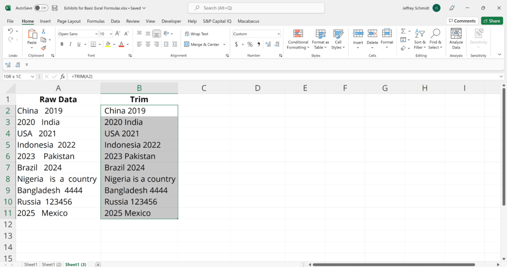
6. TRIM
The TRIM function makes sure your functions do not return errors due to extra spaces in your data. It ensures that all empty spaces are eliminated. Unlike other functions that can operate on a range of cells, TRIM only operates on a single cell. Therefore, it comes with the downside of adding duplicated data to your spreadsheet.
=TRIM(text)
Example:
TRIM(A2) – Removes empty spaces in the value in cell A2.
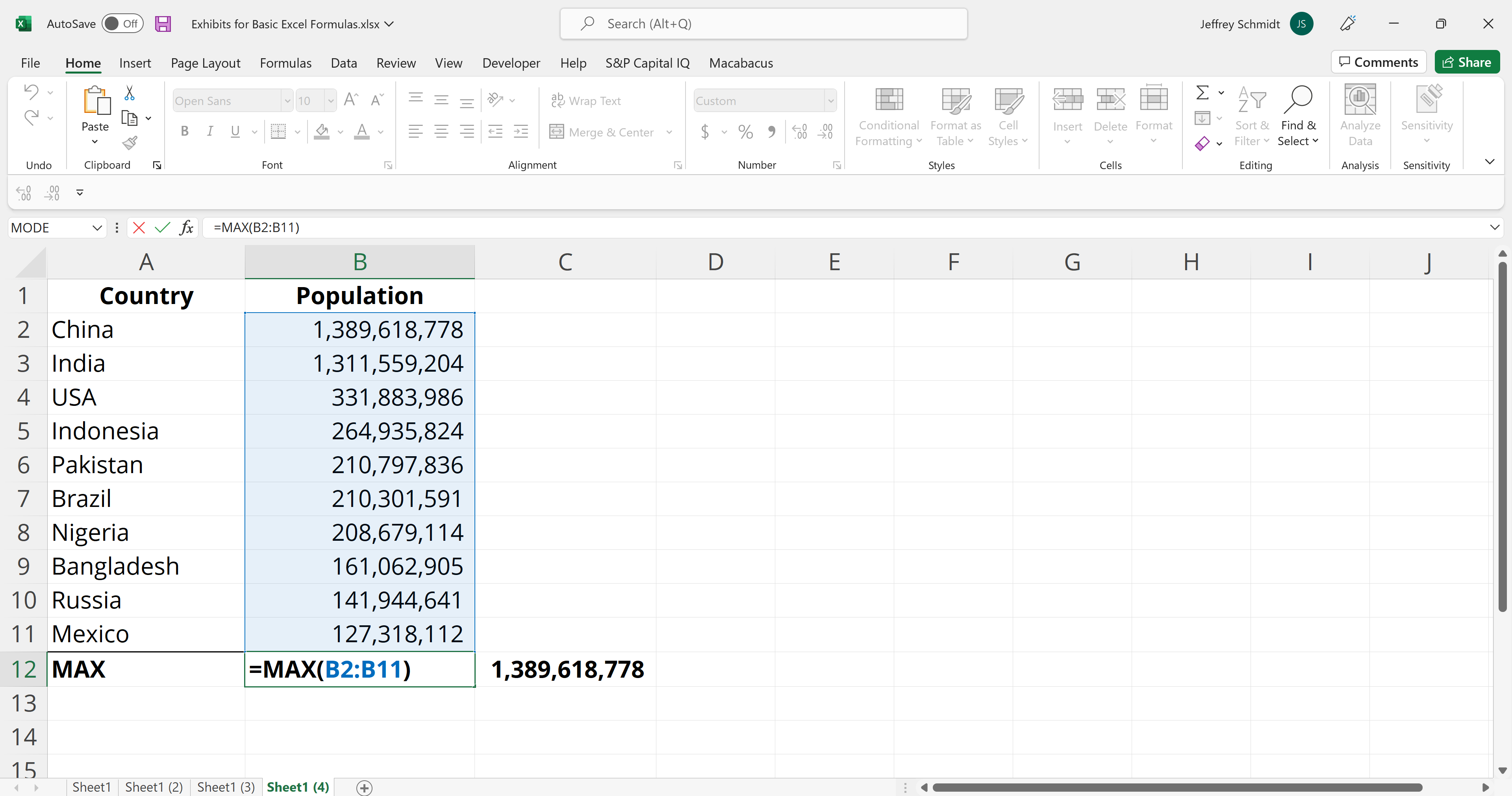
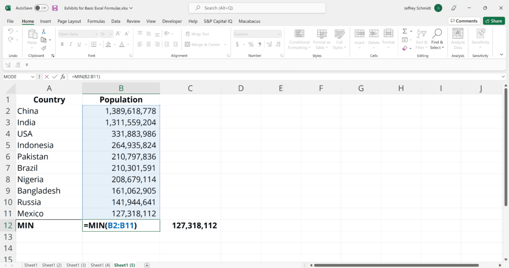
7. MAX & MIN
The MAX and MIN functions help in finding the maximum number and the minimum number in a range of values.
=MIN(number1, [number2], …)
Example:
=MIN(B2:C11) – Finds the minimum number between column B from B2 and column C from C2 to row 11 in both columns B and C.
=MAX(number1, [number2], …)
Example:
=MAX(B2:C11) – Similarly, it finds the maximum number between column B from B2 and column C from C2 to row 11 in both columns B and C.
More Resources
Thank you for reading CFI’s guide to basic Excel formulas. To continue your development as a world-class financial analyst, these additional CFI resources will be helpful:
- Advanced Excel Formulas
- Benefits of Excel Shortcuts
- Valuation Modeling in Excel
- See all Excel resources