
In a Microsoft Excel spreadsheet, values can refer to text, dates, numbers, or Boolean data. The type of value depends on the data to which it’s referring.In the case of digital spreadsheets, like Microsoft Excel, the term “number data” is used to describe numeric data instead.
Contents
- 1 What does value mean in Excel?
- 2 What is the value in a spreadsheet?
- 3 How do you use values in Excel?
- 4 Why is Excel #value?
- 5 How do you find the value in Excel?
- 6 How do u find the value?
- 7 What is label and value in Excel?
- 8 How do you use values?
- 9 How do I give text a value in Excel?
- 10 How do I make excel not show #value?
- 11 How do I fix ## in Excel?
- 12 How do you handle #value in Excel?
- 13 What is a value example?
- 14 What is the value of 3?
- 15 What is the value of 6?
- 16 What are the 3 types of data in Excel?
- 17 What are labels used for?
- 18 What are spreadsheets used for?
- 19 Does value mean worth?
- 20 Why do we need values?
What does value mean in Excel?
#VALUE is Excel’s way of saying, “There’s something wrong with the way your formula is typed. Or, there’s something wrong with the cells you are referencing.” The error is very general, and it can be hard to find the exact cause of it.
What is the value in a spreadsheet?
Values are numbers entered into spreadsheet cells. If a formula or function returns a number into a cell, this data is also a value.
How do you use values in Excel?
One quick and easy way to add values in Excel is to use AutoSum. Just select an empty cell directly below a column of data. Then on the Formula tab, click AutoSum > Sum. Excel will automatically sense the range to be summed.
The #VALUE! error appears when a value is not the expected type. This can occur when cells are left blank, when a function that is expecting a number is given a text value, and when dates are treated as text by Excel.
How do you find the value in Excel?
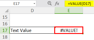
Use the VALUE function to convert text input to a numeric value. The VALUE function converts text that appears in a recognized format (i.e. a number, date, or time format) into a numeric value. Normally, Excel automatically converts text to numeric values as needed, so the VALUE function is not needed.
How do u find the value?
You can find this by adding the numbers in a set and dividing it by the number of numbers in that set. The value of a function at a certain point refers to the value of a function if you plug in the values given for the variables in the function. Value can also refer to worth of an object in math.
What is label and value in Excel?
Entering data into a spreadsheet is just like typing in a word processing program, but you have to first click the cell in which you want the data to be placed before typing the data. All words describing the values (numbers) are called labels. The numbers, which can later be used in formulas, are called values.
How do you use values?
7 Ways to Apply Your Personal Core Values in Daily Life
- Put them where you can see them.
- Discuss them with close family and friends.
- Put the right people in your life (and eliminate the wrong ones).
- Assess your daily tasks each morning.
- Integrate them into your regular conversations.
- Apply them as key motivators.
How do I give text a value in Excel?
Select the column, or range where you’ll be putting the values, then use CTRL+1 to bring up the Format > Cells dialog and on the Number tab select Text. Now Excel will keep your leading 0’s.
How do I make excel not show #value?
Hide error indicators in cells
You can prevent these indicators from being displayed by using the following procedure. In Excel 2016, Excel 2013, and Excel 2010: Click File > Options >Formulas. > Excel Options > Formulas. Under Error Checking, clear the Enable background error checking check box.
How do I fix ## in Excel?
To fix, try increasing the column width first. Drag the column marker to the right until you have doubled or even tripled the width. If the cell displays properly, adjust the width back down as needed, or apply a shorter number format.
How do you handle #value in Excel?
When there is a cell reference to an error value, IF displays the #VALUE! error. Solution: You can use any of the error-handling formulas such as ISERROR, ISERR, or IFERROR along with IF. The following topics explain how to use IF, ISERROR and ISERR, or IFERROR in a formula when your argument refers to error values.
What is a value example?
Values are standards or ideals with which we evaluate actions, people, things, or situations. Beauty, honesty, justice, peace, generosity are all examples of values that many people endorse.
What is the value of 3?
3 is in thousands place and its place value is 3,000, 5 is in hundreds place and its place value is 500, 4 is in tens place and its place value is 40, 8 is in ones place and its place value is 8.
What is the value of 6?
Since 6 is six units away towards right from 0, the absolute value of 6 is just 6. The absolute value of 6 is written as |6| and is equal to 6.
What are the 3 types of data in Excel?
You enter three types of data in cells: labels, values, and formulas. Labels (text) are descriptive pieces of information, such as names, months, or other identifying statistics, and they usually include alphabetic characters.
What are labels used for?
Labels may be used for any combination of identification, information, warning, instructions for use, environmental advice or advertising. They may be stickers, permanent or temporary labels or printed packaging.
What are spreadsheets used for?
A spreadsheet is a tool that is used to store, manipulate and analyze data. Data in a spreadsheet is organized in a series of rows and columns and can be searched, sorted, calculated and used in a variety of charts and graphs.
Does value mean worth?
1. Value, worth imply intrinsic excellence or desirability. Value is that quality of anything which renders it desirable or useful: the value of sunlight or good books. Worth implies especially spiritual qualities of mind and character, or moral excellence: Few knew her true worth.
Why do we need values?
Our values inform our thoughts, words, and actions.
Our values are important because they help us to grow and develop. They help us to create the future we want to experience.The decisions we make are a reflection of our values and beliefs, and they are always directed towards a specific purpose.
In a Microsoft Excel spreadsheet, values can refer to text, dates, numbers, or Boolean data. The type of value depends on the data to which it’s referring.
Before spreadsheet software was invented, the term «value» in relation to a spreadsheet meant only numeric data. In the case of digital spreadsheets, like Microsoft Excel, the term «number data» is used to describe numeric data instead.
Definitions in this article apply to Excel 2019, Excel 2016, 2013, and 2010, as well as Excel for Mac, Excel for Microsoft 365, and Excel Online.
Types of Values in Excel
If someone refers to a value in Excel, they may be referring to any of the following types of data:
- Text: String data, such as «High» or «Low.»
- Dates: A calendar date, such as «20-Nov-2018.»
- Numbers: Numeric data, such as 10 or 20.
- Boolean: A result of a logical comparison, such as TRUE or FALSE.
A «value» might also refer to a condition you define in a spreadsheet filter to view only data that you care about. For example, you may set a filter to see only rows where the value in column A is the name of an employee, like «Bob.»
Displayed Value vs. Actual Value
There are three things that define the value that gets displayed in a cell: the formula for that cell, cell formatting, and the result
When you view an Excel spreadsheet, you’ll see only the result in each cell. However, if you click on the cell, you’ll see the formula for that cell in the formula field at the top of the spreadsheet.
Formulas and formatting determine what results get displayed in each cell in different ways. A formula uses various Excel functions to perform a calculation. The result of that calculation is displayed in the cell. You can format cells in Excel to display values in financial, decimal, percentage, scientific, and many other formats. You can also set how many decimal points get displayed.
For example, the formula for cell A2 that divides number values in A1 and B1 would be =A1/B1 with a result of 20.154. However, you may set the formatting for cell A2 to display only two decimal points. In this case, the value in A2 would be 20.15.
Error Values
The term «value» is also associated with error values, such as #NULL!, #REF!, and #DIV/0!, which are displayed when Excel detects problems with formulas or the data in the cells they reference.
These are considered values because you can include them as arguments for some Excel functions.
For example, if you create a formula in cell B3 that divides the number in A2 by the blank cell A3, this results in the value #DIV/0!.
This is because the blank cell is treated as zero, which results in an error value #DIV/0!. This error value means «divide by zero error.»
#VALUE! Errors
Another error value is #VALUE!
This error occurs when a formula includes references to cells containing data types that are incorrect for the formula you’re using.
If you use formulas that perform an arithmetic operation such as addition, subtraction, multiplication, or division, but you reference a cell with text instead of a number, the result will be the #VALUE! error value.
For example, if you type the formula =A3/A4 where A3 contains the number 10 and A4 contains the word «Test,» the result will be #VALUE!. This is because Excel can’t divide a number by a text value.
Constant Values
Excel also has a set of special functions that return fixed values. These formulas don’t require you to reference any other cells as arguments.
Some examples include:
- PI: Returns the constant value of Pi (3.14).
- TODAY: Returns today’s date.
- RAND: Returns a random number.
The value data type returned by these functions depends on the function. For example, the TODAY() function returns a date value. The PI() function returns a decimal value.
The VALUE Function
One more definition of the term «value» in Excel is in reference to the VALUE function.
The VALUE function converts text into a number, as long as the text represents a number in some form. The input argument for the VALUE function can be text inserted directly into the function, or you can reference a cell in the spreadsheet that contains the text you want to convert.
Thanks for letting us know!
Get the Latest Tech News Delivered Every Day
Subscribe
Содержание
- Overview of formulas in Excel
- Create a formula that refers to values in other cells
- See a formula
- Enter a formula that contains a built-in function
- Download our Formulas tutorial workbook
- Formulas in-depth
- Need more help?
- How to correct a #VALUE! error
- Fix the error for a specific function
- Problems with subtraction
- Subtract a cell reference from another
- Or, use SUM with positive and negative numbers
- Subtract a cell reference from another
- Or, use the DATEDIF function
- Problems with spaces and text
- 1. Select referenced cells
- 2. Find and replace
- 3. Replace spaces with nothing
- 4. Replace or Replace all
- 5. Turn on the filter
- 6. Set the filter
- 7. Select any unnamed checkboxes
- 8. Select blank cells, and delete
- 9. Clear the filter
- 10. Result
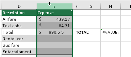
- Example with #VALUE!
- Same example, with ISTEXT
- Other solutions to try
- Select the error
- Click Formulas > Evaluate Formula
- Cell with #VALUE!
- Error hidden by IFERROR
Overview of formulas in Excel
Get started on how to create formulas and use built-in functions to perform calculations and solve problems.

Important: The calculated results of formulas and some Excel worksheet functions may differ slightly between a Windows PC using x86 or x86-64 architecture and a Windows RT PC using ARM architecture. Learn more about the differences.
Important: In this article we discuss XLOOKUP and VLOOKUP, which are similar. Try using the new XLOOKUP function, an improved version of VLOOKUP that works in any direction and returns exact matches by default, making it easier and more convenient to use than its predecessor.
Create a formula that refers to values in other cells
Type the equal sign =.
Note: Formulas in Excel always begin with the equal sign.
Select a cell or type its address in the selected cell.

Enter an operator. For example, – for subtraction.
Select the next cell, or type its address in the selected cell.

Press Enter. The result of the calculation appears in the cell with the formula.
See a formula
When a formula is entered into a cell, it also appears in the Formula bar.

To see a formula, select a cell, and it will appear in the formula bar.

Enter a formula that contains a built-in function
Select an empty cell.
Type an equal sign = and then type a function. For example, =SUM for getting the total sales.
Type an opening parenthesis (.
Select the range of cells, and then type a closing parenthesis).

Press Enter to get the result.
Download our Formulas tutorial workbook
We’ve put together a Get started with Formulas workbook that you can download. If you’re new to Excel, or even if you have some experience with it, you can walk through Excel’s most common formulas in this tour. With real-world examples and helpful visuals, you’ll be able to Sum, Count, Average, and Vlookup like a pro.
Formulas in-depth
You can browse through the individual sections below to learn more about specific formula elements.
A formula can also contain any or all of the following: functions, references, operators, and constants.
Parts of a formula

1. Functions: The PI() function returns the value of pi: 3.142.
2. References: A2 returns the value in cell A2.
3. Constants: Numbers or text values entered directly into a formula, such as 2.
4. Operators: The ^ (caret) operator raises a number to a power, and the * (asterisk) operator multiplies numbers.
A constant is a value that is not calculated; it always stays the same. For example, the date 10/9/2008, the number 210, and the text «Quarterly Earnings» are all constants. An expression or a value resulting from an expression is not a constant. If you use constants in a formula instead of references to cells (for example, =30+70+110), the result changes only if you modify the formula. In general, it’s best to place constants in individual cells where they can be easily changed if needed, then reference those cells in formulas.
A reference identifies a cell or a range of cells on a worksheet, and tells Excel where to look for the values or data you want to use in a formula. You can use references to use data contained in different parts of a worksheet in one formula or use the value from one cell in several formulas. You can also refer to cells on other sheets in the same workbook, and to other workbooks. References to cells in other workbooks are called links or external references.
The A1 reference style
By default, Excel uses the A1 reference style, which refers to columns with letters (A through XFD, for a total of 16,384 columns) and refers to rows with numbers (1 through 1,048,576). These letters and numbers are called row and column headings. To refer to a cell, enter the column letter followed by the row number. For example, B2 refers to the cell at the intersection of column B and row 2.
The cell in column A and row 10
The range of cells in column A and rows 10 through 20
The range of cells in row 15 and columns B through E
All cells in row 5
All cells in rows 5 through 10
All cells in column H
All cells in columns H through J
The range of cells in columns A through E and rows 10 through 20
Making a reference to a cell or a range of cells on another worksheet in the same workbook
In the following example, the AVERAGE function calculates the average value for the range B1:B10 on the worksheet named Marketing in the same workbook.

1. Refers to the worksheet named Marketing
2. Refers to the range of cells from B1 to B10
3. The exclamation point (!) Separates the worksheet reference from the cell range reference
Note: If the referenced worksheet has spaces or numbers in it, then you need to add apostrophes (‘) before and after the worksheet name, like =’123′!A1 or =’January Revenue’!A1.
The difference between absolute, relative and mixed references
Relative references A relative cell reference in a formula, such as A1, is based on the relative position of the cell that contains the formula and the cell the reference refers to. If the position of the cell that contains the formula changes, the reference is changed. If you copy or fill the formula across rows or down columns, the reference automatically adjusts. By default, new formulas use relative references. For example, if you copy or fill a relative reference in cell B2 to cell B3, it automatically adjusts from =A1 to =A2.
Copied formula with relative reference

Absolute references An absolute cell reference in a formula, such as $A$1, always refer to a cell in a specific location. If the position of the cell that contains the formula changes, the absolute reference remains the same. If you copy or fill the formula across rows or down columns, the absolute reference does not adjust. By default, new formulas use relative references, so you may need to switch them to absolute references. For example, if you copy or fill an absolute reference in cell B2 to cell B3, it stays the same in both cells: =$A$1.
Copied formula with absolute reference

Mixed references A mixed reference has either an absolute column and relative row, or absolute row and relative column. An absolute column reference takes the form $A1, $B1, and so on. An absolute row reference takes the form A$1, B$1, and so on. If the position of the cell that contains the formula changes, the relative reference is changed, and the absolute reference does not change. If you copy or fill the formula across rows or down columns, the relative reference automatically adjusts, and the absolute reference does not adjust. For example, if you copy or fill a mixed reference from cell A2 to B3, it adjusts from =A$1 to =B$1.
Copied formula with mixed reference

The 3-D reference style
Conveniently referencing multiple worksheets If you want to analyze data in the same cell or range of cells on multiple worksheets within a workbook, use a 3-D reference. A 3-D reference includes the cell or range reference, preceded by a range of worksheet names. Excel uses any worksheets stored between the starting and ending names of the reference. For example, =SUM(Sheet2:Sheet13!B5) adds all the values contained in cell B5 on all the worksheets between and including Sheet 2 and Sheet 13.
You can use 3-D references to refer to cells on other sheets, to define names, and to create formulas by using the following functions: SUM, AVERAGE, AVERAGEA, COUNT, COUNTA, MAX, MAXA, MIN, MINA, PRODUCT, STDEV.P, STDEV.S, STDEVA, STDEVPA, VAR.P, VAR.S, VARA, and VARPA.
3-D references cannot be used in array formulas.
3-D references cannot be used with the intersection operator (a single space) or in formulas that use implicit intersection.
What occurs when you move, copy, insert, or delete worksheets The following examples explain what happens when you move, copy, insert, or delete worksheets that are included in a 3-D reference. The examples use the formula =SUM(Sheet2:Sheet6!A2:A5) to add cells A2 through A5 on worksheets 2 through 6.
Insert or copy If you insert or copy sheets between Sheet2 and Sheet6 (the endpoints in this example), Excel includes all values in cells A2 through A5 from the added sheets in the calculations.
Delete If you delete sheets between Sheet2 and Sheet6, Excel removes their values from the calculation.
Move If you move sheets from between Sheet2 and Sheet6 to a location outside the referenced sheet range, Excel removes their values from the calculation.
Move an endpoint If you move Sheet2 or Sheet6 to another location in the same workbook, Excel adjusts the calculation to accommodate the new range of sheets between them.
Delete an endpoint If you delete Sheet2 or Sheet6, Excel adjusts the calculation to accommodate the range of sheets between them.
The R1C1 reference style
You can also use a reference style where both the rows and the columns on the worksheet are numbered. The R1C1 reference style is useful for computing row and column positions in macros. In the R1C1 style, Excel indicates the location of a cell with an «R» followed by a row number and a «C» followed by a column number.
A relative reference to the cell two rows up and in the same column
A relative reference to the cell two rows down and two columns to the right
An absolute reference to the cell in the second row and in the second column
A relative reference to the entire row above the active cell
An absolute reference to the current row
When you record a macro, Excel records some commands by using the R1C1 reference style. For example, if you record a command, such as clicking the AutoSum button to insert a formula that adds a range of cells, Excel records the formula by using R1C1 style, not A1 style, references.
You can turn the R1C1 reference style on or off by setting or clearing the R1C1 reference style check box under the Working with formulas section in the Formulas category of the Options dialog box. To display this dialog box, click the File tab.
Need more help?
You can always ask an expert in the Excel Tech Community or get support in the Answers community.
Источник
How to correct a #VALUE! error
#VALUE is Excel’s way of saying, «There’s something wrong with the way your formula is typed. Or, there’s something wrong with the cells you are referencing.» The error is very general, and it can be hard to find the exact cause of it. The information on this page shows common problems and solutions for the error. You may need to try one or more of the solutions to fix your particular error.

Fix the error for a specific function
Don’t see your function in this list? Try the other solutions listed below.
Problems with subtraction
If you’re new to Excel, you might be typing a formula for subtraction incorrectly. Here are two ways to do it:
Subtract a cell reference from another
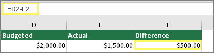
Type two values in two separate cells. In a third cell, subtract one cell reference from the other. In this example, cell D2 has the budgeted amount, and cell E2 has the actual amount. F2 has the formula =D2-E2.
Or, use SUM with positive and negative numbers
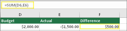
Type a positive value in one cell, and a negative value in another. In a third cell, use the SUM function to add the two cells together. In this example, cell D6 has the budgeted amount, and cell E6 has the actual amount as a negative number. F6 has the formula =SUM(D6,E6).
If you’re using Windows, you might get the #VALUE! error when doing even the most basic subtraction formula. The following might solve your problem:
First do a quick test. In a new workbook, type a 2 in cell A1. Type a 4 in cell B1. Then in C1 type this formula =B1-A1. If you get the #VALUE! error, go to the next step. If you don’t get the error, try other solutions on this page.
In Windows, open your Region control panel.
Windows 10: Click Start, type Region, and then click the Region control panel.
Windows 8: At the Start screen, type Region, click Settings, and then click Region.
Windows 7: Click Start and then type Region, and then click Region and language.
On the Formats tab, click Additional settings.
Look for the List separator. If the List separator is set to the minus sign, change it to something else. For example, a comma is a common list separator. The semicolon is also common. However, another list separator might be more appropriate for your particular region.
Open your workbook. If a cell contains a #VALUE! error, double-click to edit it.
If there are commas where there should be minus signs for subtraction, change them to minus signs.
Repeat this process for other cells that have the error.
Subtract a cell reference from another
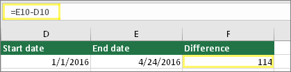
Type two dates in two separate cells. In a third cell, subtract one cell reference from the other. In this example, cell D10 has the start date, and cell E10 has the End date. F10 has the formula =E10-D10.
Or, use the DATEDIF function
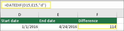
Type two dates in two separate cells. In a third cell, use the DATEDIF function to find the difference in dates. For more information on the DATEDIF function, see Calculate the difference between two dates.
Make your date column wider. If your date is aligned to the right, then it’s a date. But if it’s aligned to the left, this means the date isn’t really a date. It’s text. And Excel won’t recognize text as a date. Here are some solutions that can help this problem.
Check for leading spaces
Double-click a date that is being used in a subtraction formula.
Put your cursor at the beginning and see if you can select one or more spaces. Here’s what a selected space looks like at the beginning of a cell: 
If your cell has this problem, proceed to the next step. If you don’t see one or more spaces, go to the next section on checking your computer’s date settings.
Select the column that contains the date by clicking its column header.
Click Data > Text to Columns.
Click Next twice.
On Step 3 of 3 of the wizard, under Column data format, click Date.
Choose a date format, and then click Finish.
Repeat this process for other columns to ensure they don’t contain leading spaces before dates.
Check your computer’s date settings
Excel uses your computer’s date system. If a cell’s date isn’t entered using the same date system, then Excel won’t recognize it as a true date.
For example, let’s say that your computer displays dates as mm/dd/yyyy. If you typed a date like that in a cell, Excel would recognize it as a date and you’d be able to use it in a subtraction formula. However, if you typed a date like dd/mm/yy, then Excel wouldn’t recognize that as a date. Instead, it would treat it as text.
There are two solutions to this problem: You could change the date system that your computer uses to match the date system you want to type in Excel. Or, in Excel you could create a new column and use the DATE function to create a true date based on the date stored as text. Here’s how to do that assuming your computers date system is mm/dd/yyy and your text date is 31/12/2017 in cell A1:
Create a formula like this: =DATE(RIGHT(A1,4),MID(A1,4,2),LEFT(A1,2))
The result would be 12/31/2017.
If you want the format to appear like dd/mm/yy, press CTRL+1 (or  + 1 on the Mac).
Choose a different locale that uses the dd/mm/yy format, for example, English (United Kingdom). When you’re done applying the format, the result would be 31/12/2017 and it would be a true date, not a text date.
Note: The formula above is written with the DATE, RIGHT, MID, and LEFT functions. Please notice that it is written with an assumption that the text date has two characters for days, two characters for months, and four characters for year. You may need to customize the formula to suit your date.
Problems with spaces and text
Often #VALUE! occurs because your formula refers to other cells that contain spaces, or even trickier: hidden spaces. These spaces can make a cell look blank, when in fact they are not blank.
1. Select referenced cells
Find cells that your formula is referencing and select them. In many cases removing spaces for an entire column is a good practice because you can replace more than one space at a time. In this example, clicking the E selects the entire column.
2. Find and replace
On the Home tab, click Find & Select > Replace.
3. Replace spaces with nothing
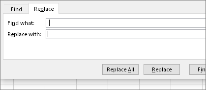
In the Find what box, type a single space. Then, in the Replace with box, delete anything that might be there.
4. Replace or Replace all
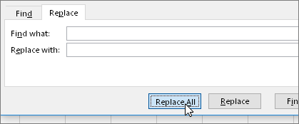
If you are confident that all spaces in the column should be removed, click Replace All. If you’d like to step through and replace spaces with nothing on an individual basis, you can click Find next first, and then click Replace when you are confident the space isn’t needed. When you’re done, the #VALUE! error may be resolved. If not, go to the next step.
5. Turn on the filter
Sometimes there are hidden characters other than spaces that can make a cell appear blank, when it’s not really blank. Single apostrophes within a cell can do this. To get rid of these characters in a column, turn on the filter by going to Home > Sort & Filter > Filter.
6. Set the filter

Click the filter arrow  , and then deselect Select all. Then, select the Blanks checkbox.
7. Select any unnamed checkboxes
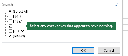
Select any check boxes that don’t have anything next to them, like this one.
8. Select blank cells, and delete

When Excel brings back the blank cells, select them. Then press the Delete key. This will clear any hidden characters in the cells.
9. Clear the filter
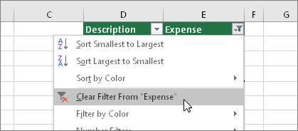
Click the filter arrow , and then click Clear filter from. so that all cells are visible.
10. Result
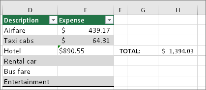
If spaces were the culprit of your #VALUE! error then hopefully your error has been replaced by the formula result, as shown here in our example. If not, repeat this process for other cells that your formula refers to. Or, try other solutions on this page.
Note: In this example, notice that cell E4 has a green triangle and the number is aligned to the left. This means the number is stored as text. This may cause more problems later. If you see this problem, we recommend converting numbers stored as text to numbers.
Text or special characters within a cell can cause the #VALUE! error. But sometimes it’s hard to see which cells have these problems. Solution: Use the ISTEXT function to inspect cells. Please note that ISTEXT doesn’t resolve the error, it simply finds cells that might be causing the error.
Example with #VALUE!
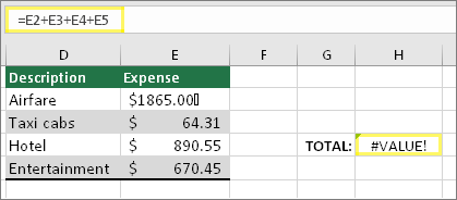
Here’s an example of a formula that has a #VALUE! error. This is likely due to cell E2. There is a special character that appears as a small box after «00.» Or as the next picture shows, you could use the ISTEXT function in a separate column to check for text.
Same example, with ISTEXT
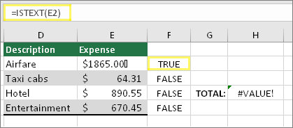
Here the ISTEXT function was added in column F. All cells are fine except the one with the value of TRUE. This means cell E2 has text. To resolve this, you could delete the cell’s contents and retype the value of 1865.00. Or you could also use the CLEAN function to clean out characters, or use the REPLACE function to replace special characters with other values.
After using CLEAN or REPLACE, you’ll want to copy the result, and use Home > Paste > Paste Special > Values. You might also have to convert numbers stored as text to numbers.
Formulas with math operations like + and * may not be able to calculate cells that contain text or spaces. In this case, try using a function instead. Functions will often ignore text values and calculate everything as numbers, eliminating the #VALUE! error. For example, instead of =A2+B2+C2, type =SUM(A2:C2). Or, instead of =A2*B2, type =PRODUCT(A2,B2).
Other solutions to try
Select the error

First select the cell with the #VALUE! error.
Click Formulas > Evaluate Formula
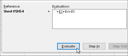
Click Formulas > Evaluate Formula > Evaluate. Excel will step through the parts of the formula individually. In this case the formula =E2+E3+E4+E5 breaks because of a hidden space in cell E2. You can’t see the space by looking at cell E2. However, you can see it here. It shows as » «.
Sometimes you just want to replace the #VALUE! error with something else like your own text, a zero or a blank cell. In this case you can add the IFERROR function to your formula. IFERROR will check to see if there’s an error, and if so, replace it with another value of your choice. If there isn’t an error, your original formula will be calculated. IFERROR will only work in Excel 2007 and later. For earlier versions you can use IF(ISERROR()).
Warning: IFERROR will hide all errors, not just the #VALUE! error. Hiding errors isn’t recommended because an error is often a sign that something needs to be fixed, not hidden. We don’t recommend using this function unless you are absolutely certain your formula works the way that you want.
Cell with #VALUE!
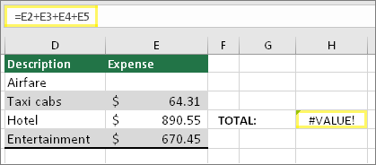
Here’s an example of a formula that has a #VALUE! error due to a hidden space in cell E2.
Error hidden by IFERROR
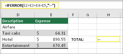
And here’s the same formula with IFERROR added to the formula. You can read the formula as: «Calculate the formula, but if there’s any kind of error, replace it with two dashes.» Note that you could also use «» to display nothing instead of two dashes. Or you could substitute your own text, such as: «Total Error».
Unfortunately, you can see that IFERROR doesn’t actually resolve the error, it simply hides it. So be certain that hiding the error is better than fixing it.
Your data connection may have become unavailable at some point. To fix this, restore the data connection, or consider importing the data if possible. If you don’t have access to the connection, ask the creator of the workbook to make a new file for you. The new file ideally would only have values, and no connections. They can do this by copying all the cells, and pasting only as values. To paste as only values, they can click Home > Paste > Paste Special > Values. This eliminates all formulas and connections, and therefore would also remove any #VALUE! errors.
If you’re not sure what to do at this point, you can search for similar questions in the Excel Community Forum, or post one of your own.
Источник
VALUE Function in Excel (Table of Contents)
- VALUE in Excel
- Step for using the VALUE Function
- How to Use VALUE Function in Excel?
Introduction to VALUE Function
The value function is one kind of text function in excel which is used for converting a text string or array, which also represents a number into a number thing. This is not actually a complete text. To understand this better, suppose we have a data set wherein a column which has currencies amount is mentioned. With the help of the Value function, we can convert that currency figure with a currency signature into a pure value by which we can conclude or use that value anywhere.
VALUE Formula in Excel:
The Formula for the VALUE Function in Excel is as follows.
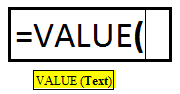
The VALUE function uses the arguments:-
There is only one argument in the VALUE Function which is mentioned below. Value (Required Argument / Text Value) – It is the text enclosed in quotation marks or a reference to a cell containing the text you want to convert.
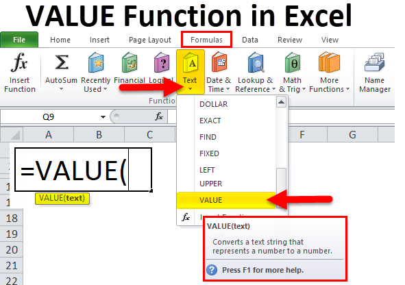
Step for using the VALUE Function
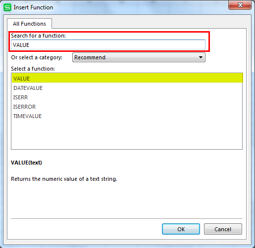
- Select the Formulas tab.
- Choose Text to open the Function drop-down list.
- Select VALUE in the list to bring up the function’s dialog box
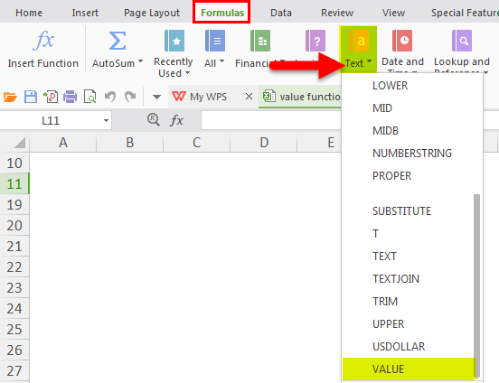
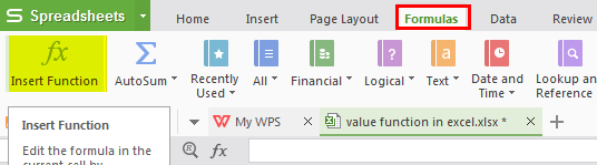
- Also, click on the Insert function icon, then manually write and search the formula
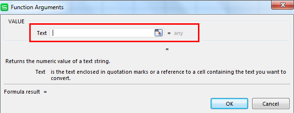
- We get a new function window showing in the below mention pictures.
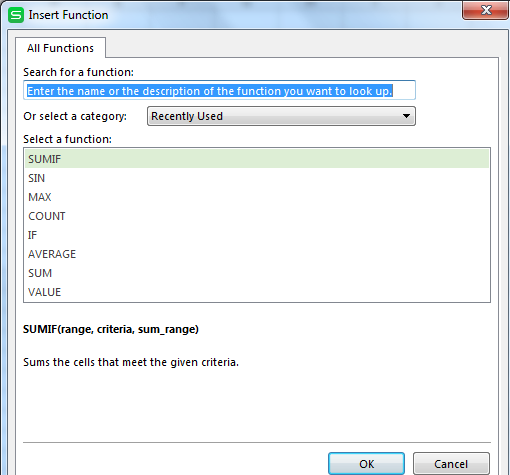
- Write the value in the open dialog box.
- Then we have to enter the details as shown in the picture.
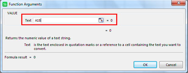
- Put the Cell value or text value where you want to convert the data type.
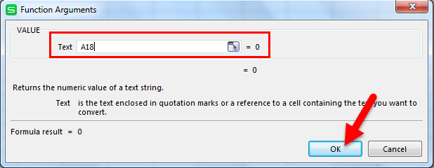
- Then Click On OK.
Shortcut for using the Formula:
Click on the cell where you want the result from value, then put the formula as mentioned below.
= Value (Cell Value / Text Value)
How to Use Value Function in Excel?
Value Function in Excel is very simple and easy to use. Let’s understand the working of Value Function in Excel by few Examples.
You can download this VALUE Function Excel Template here – VALUE Function Excel Template
Example #1
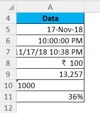
Like the above image, we have few data which is different like date, time, currency, numbers, numeric in-text value, and discount percentage; we can see below in the value function how to convert all the data as a numeric value, then you can easily make any calculations on the result value, now we are using value function formula below.
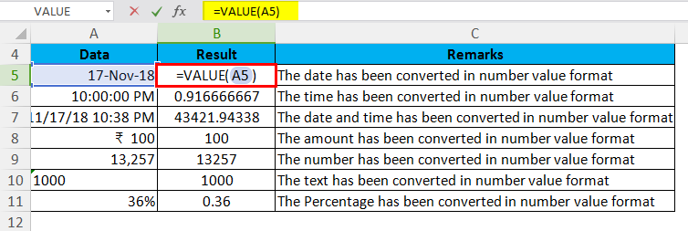
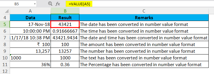
It returns the result as shown below:
Example #2
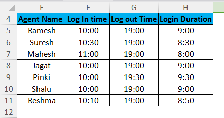
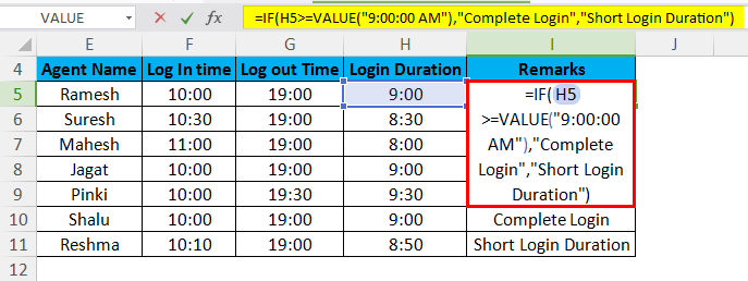
There are some details of calling agents in a call center as shown in the above table. Agent Name, Agent first log in time, Log out time. Total login duration on the system then we check with a formula which agent has not completed the login duration, so we can use the IF Function to check the same; in this formula, we take the help of value function, because we are giving the timing criteria in text format. We are using the IF Function with value function; value function converted in time format, which is given in the criteria in text format.
=IF (H5 >= VALUE ( ” 9:00:00 AM ” ), ” Complete Login ” , ” Short Login Duration ” )
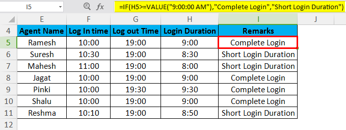
Now we can get the result as below mentioned with the help of the value function with the IF Function.
Example #3
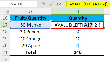
As shown in the below picture, there are names of some fruits, quantity and we want to know about the total numbers of fruits so we can get this using of value function with the left function.
=VALUE (LEFT (A17, 2))
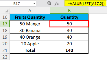
Now we can get the result like this.
Things to Remember about VALUE in Excel
- If the data is not in a format that Excel recognizes, the data can be left as text. When this situation occurs, certain functions, such as SUM or AVERAGE, ignore the data in these cells and calculation errors occur. A VALUE formula returns the #VALUE error.
- You can also track the data type by alignment; Text data aligns on the left in a cell. Numbers and dates align on the right cell.
- The function converts text that appears in a recognized format (a number in the text, date, or time format, currency, percentage ) into a numeric value.
- Normally, Excel automatically converts text to numeric values as needed, so the VALUE function is not needed regularly.
Recommended Articles
This has been a guide to VALUE in Excel. Here we discuss the VALUE Formula in Excel and how to use VALUE Function in Excel along with practical examples and downloadable excel templates. You may also look at these useful functions in excel –
- Excel DATEVALUE Function
- Excel Absolute Value
- Count Unique Values in Excel
- Excel P-Value
The VALUE function is a text function that converts a number from text format to numerical format where data is in an Excel-recognized format such as date, currency, time, etc. Mostly, if Excel recognizes a number, it automatically converts the data into numerical format. However, in other cases, we can do so using the VALUE function.
The VALUE function is most helpful when we seek compatibility with other spreadsheet programs and for using the numerical text resulting from text functions in calculations.

Syntax
The syntax of the VALUE function is quite straightforward and is given below.
=VALUE(text)
Arguments:
The VALUE function accepts only one argument, and it is mandatory.
‘text‘– This mandatory argument contains the value in text format that needs to be converted. The value of the text argument can be passed as a direct value in double quotes or as a cell reference.
Important Characteristics of the VALUE Function
Some noteworthy features of the VALUE function are as follows.
- The VALUE function only accepts the value that is recognized by Microsoft Excel such as constant number, locale formatted number, date, or time. If the value of the text argument is any value that is not recognized by Excel, the function results in a #VALUE! error.
- If the value of the text argument is empty, the VALUE function returns zero.
When using the VALUE function, it is important to note the alignment of the data as left-aligned data indicates text format whereas right-aligned data is number format.
Examples of VALUE Function
There are instances when the given data which looks like a number cannot be used further for calculations and analysis. In such scenarios, the VALUE function comes in very handy. Below are some examples to provide a better understanding of the function.
Example 1 – Simple Use of VALUE Function
In this example, we will use different types of input values for the text argument to better understand the functionality of the VALUE function.
We have taken time, date, date and time together, number in text format, and percentage as the input values. The function used is as follows.
=VALUE(B3)

In the first example, the value of the text argument is a time value which upon conversion to numerical format is transformed into the serial number. Excel stores time as fractions of a day. The VALUE function simply converted the time format to an actual serial number which can further be used in formulas.
The next example is in date format and like the time data, the VALUE function converts the date value to a sequential number as stored in Excel. The third example is a combination of date and time, and the VALUE function returns the expected result of the corresponding serial number and fraction of both date and time in cell C5.
The fourth example is a text which looks like a number. If we wish to use the data in cell B6 for any calculations, the result will also take on the text format. With the help of the VALUE function, the number is transformed from text format to numerical format.
The last example is a percentage value. The VALUE function returns the calculated numerical value of the percentage which is 0.25 in this case.
Now that the basic functionality of the VALUE function is clear, check some useful applications of the same in the examples below.
Example 2 – Converting String to Number using VALUE Function
In this scenario, we collected small donations from our neighbors to get essentials for the homeless shelter. The data collected was user-generated hence it is in text format.

To calculate the total donations received, we can extract the dollar amount and then sum it up. To segregate the donation amount from the given text, we will use the TEXTBEFORE function. It will extract the characters that occur before the dollar sign ($), which is the amount in this case. The formula used is as follows.
=TEXTBEFORE(B3,"$")
Now that the donation amount is segregated in column C, the total donation can be calculated.

Unfortunately, all the extracted data in column C is text, which is clear due to its left alignment, since the TEXTBEFORE function is a text function. Therefore, the total sum couldn’t be downloaded as seen in cell C10. To rectify this, we will use the VALUE function to convert all the data in column C into the numeric format and then calculate the total donation received. The updated formula to be used is as follows.
=VALUE(TEXTBEFORE(B3,"$"))

We can combine everything in one formula as follows.
=SUM(VALUE(TEXTBEFORE(B3:B8,"$")))

Note: One can also use the LEFT function in place of the TEXTBEFORE function to achieve the same result.
Example 3 – Converting Currency to Numerical Format
Here, in this case, we have received the monthly sales for the last year. As the sales report is from the India office, the currency formatting is different where a comma is used as a group separator in hundreds, thousands, and so on. Excel does not recognize the formatting, so it treats the sales numbers as text.

To be able to use the data for further calculations, we wish to convert them from text format to number format. As it is not an Excel-recognized format, the VALUE function will return a #VALUE! error.

To overcome this, we can first use the SUBSTITUTE function to replace all the commas with an empty string and then use the VALUE function. The formula used will be as follows.
=SUBSTITUTE(C3,",","")

Now the sales values in column D are in a recognizable format i.e. text, with the help of the VALUE function, we can convert the same in number format. Combining both steps, the final formula used will be as follows.
=VALUE(SUBSTITUTE(C3,",",""))

As evident by the right alignment of the data in column D, all the sales values are now in a number format and therefore can be further used for calculations.
Example 4 – Converting Time using the VALUE Function
In this example, we are conducting an online test where the completion time is set to 10:00 AM. However, every applicant can take extra time up to 20 minutes, but points will be assigned depending on the extra time taken which will eventually be deducted from the actual score. Here are the points to be deducted as per the completion time.

As the first step, we will calculate the extra time taken in each case. The formula used will be as follows.
=B4-$C$2

Now that we have all the values in column C, we can use the nested IF function to compare the time as per the point system and then assign the corresponding points. However, while using the delayed time data from C4:C7, we will wrap it in the VALUE function to ensure that Excel treats the time value as a number and not text.
The logic used will be as follows.
If the delayed time (C4) is less than 5 minutes, then assign 1 point, else if the delayed time is less than 10 minutes, assign 2 points….) and so on till 20 minutes. If no condition is met, the formula returns FALSE.
The formula used will be as follows.
=IF(C4<VALUE("0:05"),1,IF(C4<VALUE("0:10"),2,IF(C4<VALUE("0:15"),3,IF(C4<VALUE("0:20"),4))))

Now we have the final points that will be deducted from the final score in each case. With the help of the VALUE function, we were able to convert the time value from minutes to numerical format and execute the nested IF function.
VALUE Function vs NUMBERVALUE Function
Both the VALUE and NUMBERVALUE functions convert text that looks like a number from text format to numerical format but the NUMBERVALUE function transforms the data using the given group and decimal separators which help the function understand the format.
If the data is not in an Excel-recognized format, the VALUE function returns a #VALUE! error whereas with the NUMBERVALUE function, we can mention the group and decimal separator used in the data to convert it. Let’s understand it better using an example.

The data in cell B4 is a currency value in euros and is in a text format. The VALUE function does not recognize the data and hence throws a #VALUE! error whereas the NUMBERVALUE function converts the data from text to number format due to the mentioned decimal and group separator.
VALUE Function vs VALUETOTEXT Function
Now we know that the VALUE function converts text that looks like a number from the text format to numerical format. The VALUETOTEXT function performs the opposite conversion. The VALUETOTEXT function converts a value to text format depending on the concise or strict format.
Hopefully, now you have a clear idea about how to use the VALUE function to your advantage. Practice and discover new applications of the said function.