What are the wildcards in excel - Word и Excel - помощь в работе с программами

Excel for Microsoft 365 Excel 2021 Excel 2019 Excel 2016 Excel 2013 Excel 2010 Excel 2007 More…Less

Use wildcard characters as comparison criteria for text filters, and when you’re searching and replacing content. These can also be used in Conditional Formatting rules that use the «Format cells that contain specific text» criteria.

For more about using wildcard characters with the Find and Replace features in Excel, see Find or replace text and numbers on a worksheet.

Use	To find
? (question mark)	Any single character For example, sm?th finds «smith» and «smyth»
* (asterisk)	Any number of characters For example, *east finds «Northeast» and «Southeast»
~ (tilde) followed by ?, *, or ~	A question mark, asterisk, or tilde For example, fy06~? finds «fy06?»

Need more help?

Источник

Watch Video on Excel Wildcard Characters

There are only 3 Excel wildcard characters (asterisk, question mark, and tilde) and a lot can be done using these.

In this tutorial, I will show you four examples where these Excel wildcard characters are absolute lifesavers.

Excel Wildcard Characters – An Introduction

Wildcards are special characters that can take any place of any character (hence the name – wildcard).

There are three wildcard characters in Excel:

* (asterisk) – It represents any number of characters. For example, Ex* could mean Excel, Excels, Example, Expert, etc.
? (question mark) – It represents one single character. For example, Tr?mp could mean Trump or Tramp.
~ (tilde) – It is used to identify a wildcard character (~, *, ?) in the text. For example, let’s say you want to find the exact phrase Excel* in a list. If you use Excel* as the search string, it would give you any word that has Excel at the beginning followed by any number of characters (such as Excel, Excels, Excellent). To specifically look for excel*, we need to use ~. So our search string would be excel~*. Here, the presence of ~ ensures that excel reads the following character as is, and not as a wildcard.

Note: I have not come across many situations where you need to use ~. Nevertheless, it is a good to know feature.

Now let’s go through four awesome examples where wildcard characters do all the heavy lifting.

Now let’s look at four practical examples where Excel wildcard characters can be mighty useful:

Filtering data using a wildcard character.
Partial Lookup using wildcard character and VLOOKUP.
Find and Replace Partial Matches.
Count Non-blank cells that contain text.

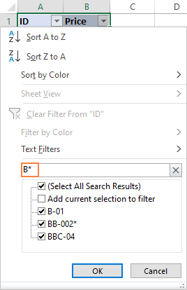
#1 Filter Data using Excel Wildcard Characters

Excel wildcard characters come in handy when you have huge data sets and you want to filter data based on a condition.

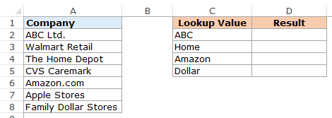
Suppose you have a dataset as shown below:

You can use the asterisk (*) wildcard character in data filter to get a list of companies that start with the alphabet A.

Here is how to do this:

This will instantly filter the results and give you 3 names – ABC Ltd., Amazon.com, and Apple Stores.

How does it work? – When you add an asterisk (*) after A, Excel would filter anything that starts with A. This is because an asterisk (being an Excel wildcard character) can represent any number of characters.

Now with the same methodology, you can use various criteria to filter results.

For example, if you want to filter companies that begin with the alphabet A and contain the alphabet C in it, use the string A*C. This will give you only 2 results – ABC Ltd. and Amazon.com.

If you use A?C instead, you will only get ABC Ltd as the result (as only one character is allowed between ‘a’ and ‘c’)

Note: The same concept can also be applied when using Excel Advanced Filters.

#2 Partial Lookup Using Wildcard Characters & VLOOKUP

Partial look-up is needed when you have to look for a value in a list and there isn’t an exact match.

For example, suppose you have a data set as shown below, and you want to look for the company ABC in a list, but the list has ABC Ltd instead of ABC.

You can not use the regular VLOOKUP function in this case as the lookup value does not have an exact match.

If you use VLOOKUP with an approximate match, it will give you the wrong results.

However, you can use a wildcard character within VLOOKUP function to get the right results:

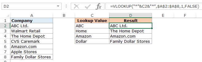
Enter the following formula in cell D2 and drag it for other cells:

=VLOOKUP("*"&C2&"*",$A$2:$A$8,1,FALSE)

How does this formula work?

In the above formula, instead of using the lookup value as is, it is flanked on both sides with the Excel wildcard character asterisk (*) – “*”&C2&”*”

This tells excel that it needs to look for any text that contains the word in C2. It could have any number of characters before or after the text in C2.

Hence, the formula looks for a match, and as soon as it gets a match, it returns that value.

3. Find and Replace Partial Matches

Excel Wildcard characters are quite versatile.

You can use it in a complex formula as well as in basic functionality such as Find and Replace.

Suppose you have the data as shown below:

In the above data, the region has been entered in different ways (such as North-West, North West, NorthWest).

This is often the case with sales data.

To clean this data and make it consistent, we can use Find and Replace with Excel wildcard characters.

Here is how to do this:

Select the data where you want to find and replace text.
Go to Home –> Find & Select –> Go To. This will open the Find and Replace dialogue box. (You can also use the keyboard shortcut – Control + H).
Enter the following text in the find and replace dialogue box:
- Find what: North*W*
- Replace with: North-West
Click on Replace All.

This will instantly change all the different formats and make it consistent to North-West.

How does this Work?

In the Find field, we have used North*W* which will find any text that has the word North and contains the alphabet ‘W’ anywhere after it.

Hence, it covers all the scenarios (NorthWest, North West, and North-West).

Find and Replace finds all these instances and changes it to North-West and makes it consistent.

4. Count Non-blank Cells that Contain Text

I know you are smart and you thinking that Excel already has an inbuilt function to do this.

You’re absolutely right!!

This can be done using the COUNTA function.

BUT… There is one small problem with it.

A lot of times when you import data or use other people’s worksheet, you will notice that there are empty cells while that might not be the case.

These cells look blank but have =”” in it. The trouble is that the

The trouble is that the COUNTA function does not consider this as an empty cell (it counts it as text).

See the example below:

In the above example, I use the COUNTA function to find cells that are not empty and it returns 11 and not 10 (but you can clearly see only 10 cells have text).

The reason, as I mentioned, is that it doesn’t consider A11 as empty (while it should).

But that is how Excel works.

The fix is to use the Excel wildcard character within the formula.

Below is a formula using the COUNTIF function that only counts cells that have text in it:

=COUNTIF(A1:A11,"?*")

This formula tells excel to count only if the cell has at least one character.

In the ?* combo:

? (question mark) ensures that at least one character is present.
* (asterisk) makes room for any number of additional characters.

Note: The above formula works when only have text values in the cells. If you have a list that has both text as well as numbers, use the following formula:

=COUNTA(A1:A11)-COUNTBLANK(A1:A11)

Similarly, you can use wildcards in a lot of other Excel functions, such as IF(), SUMIF(), AVERAGEIF(), and MATCH().

It’s also interesting to note that while you can use the wildcard characters in the SEARCH function, you can’t use it in FIND function.

Hope these examples give you a flair of the versatility and power of Excel wildcard characters.

If you have any other innovative way to use it, do share it with me in the comments section.

You May Find the Following Excel Tutorials Useful:

Using COUNTIF and COUNTIFS with Multiple Criteria.
Creating a Drop Down List in Excel.
Intersect Operator in Excel

Источник

Excel Wildcard Characters

Wildcards in Excel are the special Excel characters that take the place of the characters in it. Excel has three wildcards: an asterisk, question mark, and tilde. Asterisk is used for multiple numbers of characters in Excel, while a question mark represents only a single character. In contrast, the tilde is the identification of the wild card character.

Wildcard characters are special characters used to find the result, which is less than exact or accurate.

For example, if you have the word “Simple Chat.” In the database, you have “Simply Chat,” then the common letter in these two words is “Chat,” so we can match these with Excel wildcard characters.

Excel Wildcard Characters
- Types
  - Type #1 – Asterisk (*)
  - Type #2 – Question Mark (?)
  - Type #3 – Tilde (~)
- Examples
  - Example #1 – Usage of Excel Wildcard Character Asterisk (*)
  - Example #2 – Partial Lookup Value in VLOOKUP
  - Example #3 – Usage of Excel Wildcard Character Question Mark (?)
- Recommended Articles

You are free to use this image on your website, templates, etc, Please provide us with an attribution linkArticle Link to be Hyperlinked
For eg:
Source: Wildcard in Excel (wallstreetmojo.com)

Types

There are three types of wildcard characters in Excel.

Type #1 – Asterisk (*)

It is to match zero or the number of characters. So, for example, “Fi*” could match “Final, Fitting, Fill, Finch, and Fiasco,” etc.

Type #2 – Question Mark (?)

It is used to match any single character. For example, “Fa? e” could match “Face” & “Fade,” “?ore” could match “Bore” & “Core,” “a? ide,” which could match “Abide” and “Aside.”

Type #3 – Tilde (~)

It is used to match wildcard characters in the word. So, for example, if you have the word “Hello*” to find this word, we need to frame the sentence as “Hello~*.” So here, the character tilde (~) specifies the word “Hello” as the wildcard character does not follow it.

Examples

Example #1 – Usage of Excel Wildcard Character Asterisk (*)

You can download this Wildcard Character Excel Template here – Wildcard Character Excel Template

As we discussed, an asterisk is used to match any number of characters in the sentence.

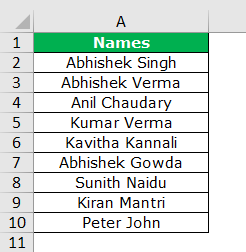
Look at the below data.
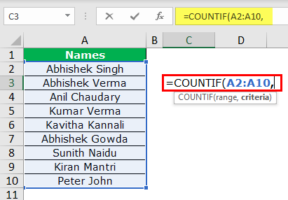
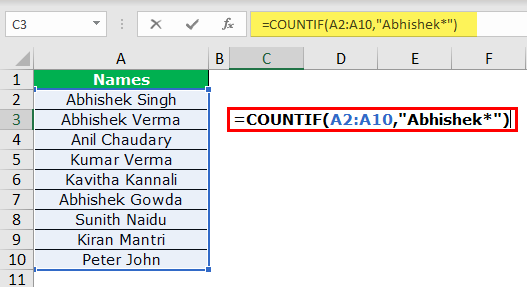
In the above data, we have names. With these names, we have many names with the common word “Abhishek.” So, using a wildcard asterisk, we can count all the “Abhishek” here. Open the COUNTIF function and select the range.
In the criteria argument, mention the criteria as “Abhishek*.”
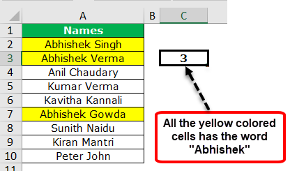
That is all. It will count all the words “Abhishek” in them.

Example #2 – Partial Lookup Value in VLOOKUP

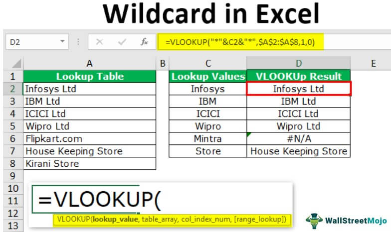
VLOOKUP requires an exact lookup_value to be matched to fetch the data. It is the traditional slogan, but we can still fetch the data using particle lookup_value. So, for example, if the lookup value is “VIVO” and in the main table, if it is “VIVO Mobile,” we can still match using wildcard characters. We will see one of the examples now. Below is the example data.

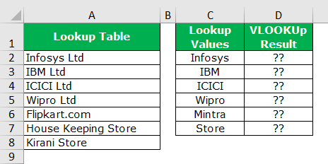
We have a lookup table in column A. In column C, we have lookup values. These lookup values are not the same as the lookup table values. So, we will see how to apply VLOOKUP using wildcards.

First, open the VLOOKUP functionThe VLOOKUP excel function searches for a particular value and returns a corresponding match based on a unique identifier. A unique identifier is uniquely associated with all the records of the database. For instance, employee ID, student roll number, customer contact number, seller email address, etc., are unique identifiers.
read more in the D1 cell.

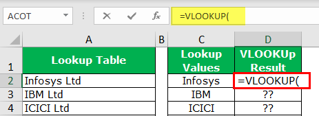
The first argument is the lookup value. One of the problems with the lookup value here is we do not have an exact match, so we need to enclose this lookup value with an asterisk before and after the lookup value.

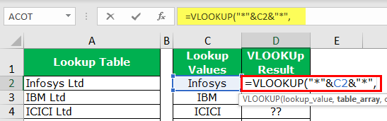
We have applied two asterisk characters, “*” &C2&”*.” Here, an asterisk indicates that we should match anything between the wildcard, and it should return the related result.

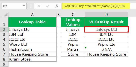
Even though we had just “Infosys,” the asterisk character matched the value in the lookup table and returned the exact result as “Infosys Ltd.”

Similarly, in cell D6, we got the error value as #VALUE#VALUE! Error in Excel represents that the reference cell the user has either entered an incorrect formula or used a wrong data type (mostly numerical data). Sometimes, it is difficult to identify the kind of mistake behind this error.read more! Because there is no word “Mintra” in the lookup tableLookup tables are simply named tables that are used in combination with the VLOOKUP function to find any data in a large data set. We can select the table and name it, and then type the table’s name instead of the reference to look up the value.read more.

Example #3 – Usage of Excel Wildcard Character Question Mark (?)

As we discussed, the question mark can match a single character in the specified slot. For example, look at the below data.

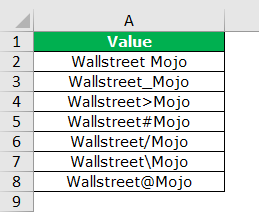
In the above data, our ideal value should be “Wallstreet Mojo,” but we have several special characters in between. So, we will use the question mark to replace all of those.

Select the data and press “Ctrl + H.”

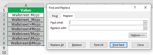
In the “Find what” box, type “Wallstreet?Mojo.” In the “Replace with” box, type “Wallstreet Mojo.”

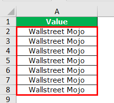
Click on Replace All. We will get the below result.

Nice, isn’t it??

The trick is done here by Excel wildcard character question mark (?). First, let us take a look at what we have mentioned.

Find What: “Wallstreet?Mojo”

Replace With: “Wallstreet Mojo”

So, after the word Wallstreet any character that the space character should replace. So, all the special characters are replaced by a space character, and we will have a proper value of “Wallstreet Mojo.”

Like this, by using wildcard characters, we can match partial data and get the job done.

Excel wildcards

What are the wildcards in Excel?
How do you use wildcards in Excel?
Can I use wildcards in IF statements in Excel?
How do you use wildcards?
What are the 5 functions in Excel?
What is * in Excel formula?
Can you use wildcards in Vlookup?
How do I use a wildcard in VBA?
How do I use Countifs with wildcard characters?
How do you use wildcards in if function?
How if function works in Excel?
How do you do an if contains in Excel?

What are the wildcards in Excel?

There are three wildcard characters in Excel:

* (asterisk) – It represents any number of characters. For example, Ex* could mean Excel, Excels, Example, Expert, etc.
? (question mark) – It represents one single character. .

(tilde) – It is used to identify a wildcard character (

How do you use wildcards in Excel?

Excel has 3 wildcards you can use in your formulas:

Asterisk (*) — zero or more characters.
Question mark (?) — any one character.
Tilde (

) — escape for literal character (

*) a literal question mark (

?), or a literal tilde (

Can I use wildcards in IF statements in Excel?

Unlike several other frequently used functions, the IF function does not support wildcards. However, you can use the COUNTIF or COUNTIFS functions inside the logical test of IF for basic wildcard functionality.

How do you use wildcards?

To use a wildcard character within a pattern: Open your query in Design view. In the Criteria row of the field that you want to use, type the operator Like in front of your criteria. Replace one or more characters in the criteria with a wildcard character.

What are the 5 functions in Excel?

To help you get started, here are 5 important Excel functions you should learn today.

The SUM Function. The sum function is the most used function when it comes to computing data on Excel. .
The TEXT Function. .
The VLOOKUP Function. .
The AVERAGE Function. .
The CONCATENATE Function.

What is * in Excel formula?

This formula sums the amounts in column D when a value in column C contains «*». The SUMIF function supports wildcards. An asterisk (*) means «one or more characters», while a question mark (?)

Can you use wildcards in Vlookup?

The VLOOKUP function supports wildcards, which makes it possible to perform a partial match on a lookup value. . To use wildcards with VLOOKUP, you must specify exact match mode by providing FALSE or 0 for the last argument, which is called range_lookup.

How do I use a wildcard in VBA?

Below are the wildcards we use in VBA LIKE operator.

Question Mark (?): This is used to match any one character from the string. .
Asterisk (*): This matches zero or more characters. .
Brackets ([]): This matches any one single character specified in the brackets.

How do I use Countifs with wildcard characters?

How to use COUNTIFS with wildcard characters

Question mark (?) — matches any single character, use it to count cells starting and/or ending with certain characters.
Asterisk (*) — matches any sequence of characters, you use it to count cells containing a specified word or a character(s) as part of the cell’s contents.

How do you use wildcards in if function?

IF function is logic test excel function. IF function tests a statement and returns values based on the result. Question mark (?) : This wildcard is used to search for any single character. Asterisk (*): This wildcard is used to find any number of characters preceding or following any character.

How if function works in Excel?

Use the IF function, one of the logical functions, to return one value if a condition is true and another value if it’s false. For example: =IF(A2>B2,»Over Budget»,»OK») =IF(A2=B2,B4-A4,»»)

How do you do an if contains in Excel?

There’s no CONTAINS function in Excel.

To find the position of a substring in a text string, use the SEARCH function. .
Add the ISNUMBER function. .
You can also check if a cell contains specific text, without displaying the substring. .
To perform a case-sensitive search, replace the SEARCH function with the FIND function.

Источник

Wildcard

A wildcard is a special character that lets you perform «fuzzy» matching on text in your Excel formulas. For example, this formula:

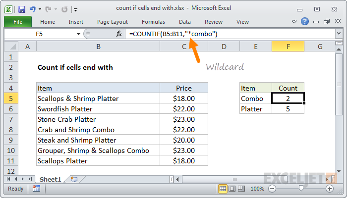
counts all cells in the range B5:B11 that end with the text «combo». And this formula:

Counts all cells in A1:A100 that contain exactly 3 characters.

Available wildcards

Excel has 3 wildcards you can use in your formulas:

Asterisk (*) — zero or more characters
Question mark (?) — any one character
Tilde (

) — escape for literal character (

*) a literal question mark (

?), or a literal tilde (

Example wildcard usage

Usage	Behavior	Will match
?	Any one character	«A», «B», «c», «z», etc.
??	Any two characters	«AA», «AZ», «zz», etc.
.	Any three characters	«Jet», «AAA», «ccc», etc.
*	Any characters	«apple», «APPLE», «A100», etc.
*th	Ends in «th»	«bath», «fourth», etc.
c*	Starts with «c»	«Cat», «CAB», «cindy», «candy», etc.
?*	At least one character	«a», «b», «ab», «ABCD», etc.
. -??	5 characters with hypen	«ABC-99″,»100-ZT», etc.
*

? Ends in question mark «Hello?», «Anybody home?», etc. *xyz* Contains «xyz» «code is XYZ», «100-XYZ», «XyZ90», etc.

Wildcards only work with text. For numeric data, you can use logical operators.

Functions that support wildcards

Not all functions allow wildcards. Here is a list of the most common functions that do:

Источник

How To Use Wildcard In Excel?

Excel has 3 wildcards you can use in your formulas:

Asterisk (*) – zero or more characters.
Question mark (?) – any one character.
Tilde (

) – escape for literal character (

*) a literal question mark (

?), or a literal tilde (

What is wildcard in Excel?

Wildcard characters in Excel are special characters that can be used to take the place of characters in a formula. They are employed in Excel formulas for incomplete matches. Excel supports wildcard characters in formulas to return values that share the same pattern.

How do you use wildcard characters?

The CHARLIST is enclosed in brackets ([ ]) and can be used with wildcard characters for more specific matches.
Examples of wildcard character pattern matching in expressions.

C haracter(s)	Use to match
? or _ (underscore)	Any single character
* or %	Zero or more characters

How do I use Asterisk in Excel?

The tilde causes Excel to handle the next character literally. In this case we are using “

*” to match a literal asterisk, but this is surrounded by asterisks on either side, in order to match an asterisk anywhere in the cell. If you just want to match an asterisk at the end of a cell, use: “*

*” for the criteria.

How do I filter wildcards in Excel?

#1 Filter Data using Excel Wildcard Characters

Select the cells that you want to filter.
Go to Data –> Sort and Filter –> Filter (Keyboard Shortcut – Control + Shift + L).
Click on the filter icon in the header cell.
In the field (below the Text Filter option), type A*
Click OK.

Why is my wildcard not working Excel?

Make sure your data doesn’t contain erroneous characters. When counting text values, make sure the data doesn’t contain leading spaces, trailing spaces, inconsistent use of straight and curly quotation marks, or nonprinting characters. In these cases, COUNTIF might return an unexpected value.

How do I find and replace wildcard characters in Excel?

Replacing a wildcard character

Press Ctrl + H to open the Find and Replace window.
Press Replace.
If we didn’t use tilde and asterisk (

*), just asterisk (*) the result would be like this.

Excel would treat asterisk as any number of characters (all the text in a cell) and convert it to a word in replace with.

How do you use wildcards to search files and folders?

You can use your own wildcards to limit search results. You can use a question mark (?) as a wildcard for a single character and an asterisk (*) as a wildcard for any number of characters. For example, *. pdf would return only files with the PDF extension.

Can you use a wildcard in an Excel IF statement?

Unlike several other frequently used functions, the IF function does not support wildcards. However, you can use the COUNTIF or COUNTIFS functions inside the logical test of IF for basic wildcard functionality.

How do I filter special characters in Excel?

Re: how to filter special characters in Excel
You can use ‘custom filter’ option available in filter option to find text with special characters. You just need to place

before the special character you want to filter.

What does * mean in Excel formula?

In Excel formula, the symbol “*” means multiplication. Say cell A1 contains 5 and cell A2 contains 8.

How do you do a Vlookup with wildcards in Excel?

To use wildcards with VLOOKUP, you must specify exact match mode by providing FALSE or 0 (zero) for the last argument called range_lookup. This expression joins the text in the named range value with a wildcard using the ampersand (&) to concatenate.

How do you use if and?

When you combine each one of them with an IF statement, they read like this:

AND – =IF(AND(Something is True, Something else is True), Value if True, Value if False)
OR – =IF(OR(Something is True, Something else is True), Value if True, Value if False)
NOT – =IF(NOT(Something is True), Value if True, Value if False)

What are wildcards in Windows 10?

The asterisk (*) and question mark (?) are used as wildcard characters, as they are in MS-DOS and Windows. The asterisk matches any sequence of characters, whereas the question mark matches any single character.

How many wild characters are present for searching files folder?

There are two wildcard characters: asterisk (*) and question mark (?). Asterisk (*) – Use the asterisk as a substitute for zero or more characters. e.g., friend* will locate all files and folders that begin with friend. Question mark (?)- Use the question mark as a substitute for a single character in a file name.

How do I search for an exact phrase in Windows 10?

To be able to locate exact phrases, you can try entering the phrase twice in quotes. For example, type “search windows” “search windows” to get all the files containing the phrase search windows. Typing “search windows” will only give you all the files containing search or windows.

How do I match a string in Excel?

Compare two strings

=A1=A2 // returns TRUE.
=EXACT(A1,A2) // returns FALSE.
=IF(EXACT(A2,A2),”Yes”,”No”)

How do you match a name in Excel where it is spelling different?

To match spelling different names, you can use the basic not equal sign ‘<>‘.

First, select the cell where you want to show the spelling differs names.
Here, I selected the H5 cell to place the result.
Now, you can write the formula in the formula bar or into your selected cell.
Type the formula. =B5<>E5.

How do I write regex in Excel?

The methods we can use are:

Test – check if the pattern can be found in the string. Returns True if it is found, False if it isn’t.
Execute – returns occurrences of the pattern matched against the string.
Replace – replaces occurrences of the pattern in the string.

How do I get UTF 8 characters in Excel?

View Unicode characters in Excel:

Open Excel from your menu or Desktop.
Navigate to Data → Get External Data → From Text.
Navigate to the location of the CSV file you want to import.
Choose the Delimited option.
Set the character encoding File Origin to 65001: Unicode (UTF-8) from the drop-down list.

Источник

Excel wildcard: find and replace, filter, use in formulas

by Svetlana Cheusheva, updated on March 14, 2023

Everything you need to know about wildcards on one page: what they are, how to best use them in Excel, and why wildcards are not working with numbers.

When you are looking for something but not exactly sure exactly what, wildcards are a perfect solution. You can think of a wildcard as a joker that can take on any value. There are only 3 wildcard characters in Excel (asterisk, question mark, and tilde), but they can do so many useful things!

Excel wildcard characters

In Microsoft Excel, a wildcard is a special kind of character that can substitute any other character. In other words, when you do not know an exact character, you can use a wildcard in that place.

The two common wildcard characters that Excel recognizes are an asterisk (*) and a question mark (?). A tilde (

) forces Excel to treat theses as regular characters, not wildcards.

Wildcards come handy in any situation when you need a partial match. You can use them as comparison criteria for filtering data, to find entries that have some common part, or to perform fuzzy matching in formulas.

Asterisk as a wildcard

The asterisk (*) is the most general wildcard character that can represent any number of characters. For example:

ch* — matches any word that begins with «ch» such as Charles, check, chess, etc.
*ch — substitutes any text string that ends with «ch» such as March, inch, fetch, etc.
*ch* — represents any word that contains «ch» in any position such as Chad, headache, arch, etc.

Question mark as a wildcard

The question mark (?) represents any single character. It can help you get more specific when searching for a partial match. For example:

? — matches any entry containing one character, e.g. «a», «1», «-«, etc.
?? — substitutes any two characters, e.g. «ab», «11», «a*», etc.
. -. — represents any string containing 2 groups of 3 characters separated with a hyphen such as ABC-DEF, ABC-123, 111-222, etc.
pri?e — matches price, pride, prize, and the like.

Tilde as a wildcard nullifier

) placed before a wildcard character cancels the effect of a wildcard and turns it into a literal asterisk (

*), a literal question mark (

?), or a literal tilde (

? — finds any entry ending with question mark, e.g. What?, Anybody there?, etc.
*

** — finds any data containing an asterisk, e.g. *1, *11*, 1-Mar-2020*, etc. In this case, the 1 st and 3 rd asterisks are wildcards, while the second one denotes a literal asterisk character.

Find and replace wildcards in Excel

The uses of wildcard characters with Excel’s Find and Replace feature are quite versatile. The following examples will discuss a few common scenarios and warn you about a couple of caveats.

How to search with wildcard

By default, the Find and Replace dialog is configured to look for the specified criteria anywhere in a cell, not to match the entire cell contents. For example, if you use «AA» as your search criteria, Excel will return all the entries containing it such as AA-01, 01-AA, 01-AA-02, and so on. That works great in most situations, but under certain circumstances can be a complication.

In the below dataset, supposing you want to find the IDs that consist of 4 characters separated with a hyphen. So, you open the Find and Replace dialog (Ctrl + F) , type ??-?? in the Find what box, and press Find All. The result looks a bit perplexing, isn’t it?

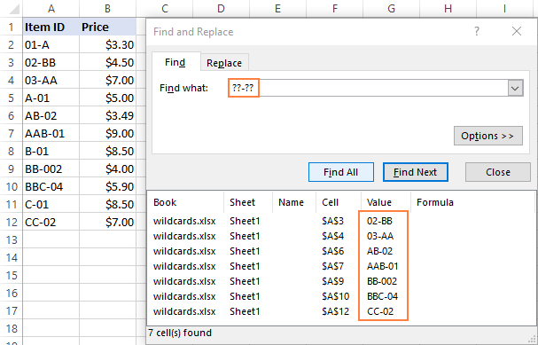
Technically, strings like AAB-01 or BB-002 also match the criteria because they do contain a ??-?? substring. To exclude these from the results, click the Options button, and check the Match entire cell contents box. Now, Excel will limit the results to only the ??-?? strings: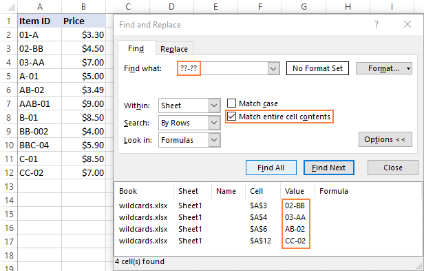

How to replace with wildcard

In case your data contains some fuzzy matches, wildcards can help you quickly locate and unify them.

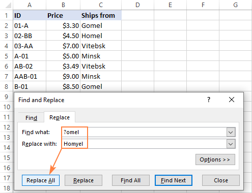
In the screenshot below, you can see two spelling variations of the same city Homel and Gomel. We’d like to replace both with another version — Homyel. (And yes, all three spellings of my native city are correct and generally accepted 🙂

To replace partial matches, this is what you need to do:

Press Ctrl + H to open the Replace tab of the Find and Replace dialog.
In the Find what box, type the wildcard expression: ?omel
In the Replace with box, type the replacement text: Homyel
Click the Replace All button.

And observe the results: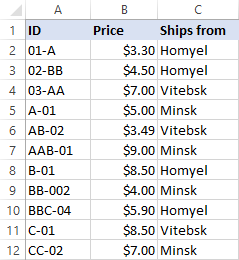

How to find and replace wildcard characters

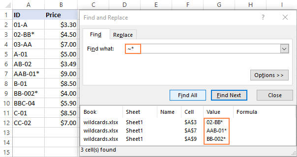
To find a character that Excel recognizes as a wildcard, i.e. a literal asterisk or question mark, include a tilde (

) in your search criteria. For example, to find all the entries containing asterisks, type

* in the Find what box:

If you’d like to replace the asterisks with something else, switch to the Replace tab and type the character of interest in the Replace with box. To remove all the found asterisk characters, leave the Replace with box empty, and click Replace all.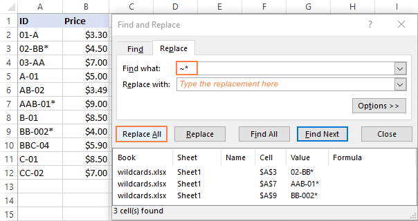

Filter data with wildcards in Excel

Excel wildcards also come very useful when you have a huge column of data and wish to filter that data based on condition.

In our sample data set, supposing you want to filter the IDs beginning with «B». For this, do the following:

Add filter to the header cells. The fastest way is to press the Ctrl + Shift + L shortcut.
In the target column, click the filter drop-down arrow.
In the Search box, type your criteria, B* in our case.
Click OK.

This will instantly filter the data based on your wildcard criteria like show below:

Wildcards can also be used with Advanced Filter, which could make it a nice alternative to regular expressions (also called regexes by tech gurus) that Excel does not support. For more information, please see Excel Advanced Filter with wildcards.

Excel formulas with wildcard

First off, it should be noted that quite a limited number of Excel functions support wildcards. Here is a list of the most popular functions that do with formula examples:

AVERAGEIF with wildcards — finds the average (arithmetic mean) of the cells that meet the specified condition.

AVERAGEIFS — returns the average of the cells that meet multiple criteria. Like AVERAGEIF in the above example allows wildcards.

COUNTIF with wildcard characters — counts the number of cells based on one criterion.

COUNTIFS with wildcards — counts the number of cells based on multiple criteria.

SUMIF with wildcard- sums cells with condition.

SUMIFS — adds cells with multiple criteria. Like SUMIF in the above example accepts wildcard characters.

VLOOKUP with wildcards — performs a vertical lookup with partial match.

HLOOKUP with wildcard — does a horizontal lookup with partial match.

XLOOKUP with wildcard characters — performs a partial match lookup both in a column and a row.

MATCH formula with wildcards — finds a partial match and returns its relative position.

XMATCH with wildcards — a modern successor of the MATCH function that also supports wildcard matching.

SEARCH with wildcards — unlike the case-sensitive FIND function, case-insensitive SEARCH understands wildcard characters.

If you need to do partial matching with other functions that do not support wildcards, you will have to figure out a workaround like Excel IF wildcard formula.

The following examples demonstrate some general approaches to using wildcards in Excel formulas.

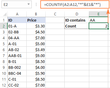
Excel COUNTIF wildcard formula

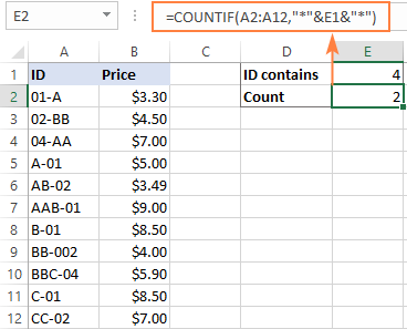
Let’s say you wish to count the number of cells containing the text «AA» in the range A2:A12. There are three ways to accomplish this.

The easiest one is to include wildcard characters directly in the criteria argument:

In practice, such «hardcoding» is not the best solution. If the criteria changes at a later point, you’ll have to edit your formula every time.

Instead of typing the criteria in the formula, you can input it in some cell, say E1, and concatenate the cell reference with the wildcard characters. Your complete formula would be:

=COUNTIF(A2:A12,»*»&E1&»*»)

Alternatively, you can input a wildcard string (*AA* in our example) in the criteria cell (E1) and include only the cell reference in the formula:

=COUNTIF(A2:A12, E1)

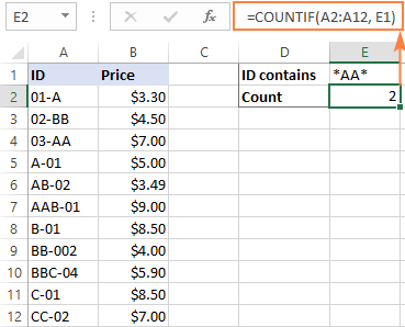
All three formulas will produce the same result, so which one to use is a matter of your personal preference.

Note. The wildcard search is not case sensitive, so the formula counts both upper case and lowercase characters like AA-01 and aa-01.

Excel wildcard VLOOKUP formula

When you need to look for a value that does not have an exact match in the source data, you can use wildcard characters to find a partial match.

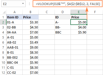
In this example, we are going to look up the IDs that start with specific characters, and return their prices from column B. To have it done, enter the unique parts of the targets IDs in cells D2, D3 and D4 and use this formula to get the results:

=VLOOKUP(D2&»*», $A$2:$B$12, 2, FALSE)

The above formula goes to E1, and due to the clever use of relative and absolute cells references it copies correctly to the below cells.

Note. As the Excel VLOOKUP function returns the first found match, you should be very careful when searching with wildcards. If your lookup value matches more than one value in the lookup range, you may get misleading results.

Excel wildcard for numbers

It is sometimes stated that wildcards in Excel only work for text values, not numbers. However, this is not exactly true. With the Find and Replace feature as well as Filter, wildcards work fine for both text and numbers.

Find and Replace with wildcard number

In the screenshot below, we are using *4* for the search criteria to search for the cells containing the digit 4, and Excel finds both text strings and numbers: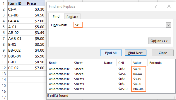

Filter with wildcard number

Likewise, Excel’s auto-filter has no problem with filtering numbers containing «4»: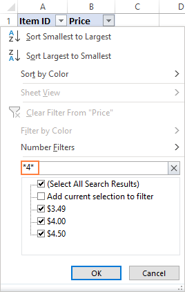

Why Excel wildcard not working with numbers in formulas

Wildcards with numbers in formulas is a different story. Using wildcard characters together with numbers (no matter whether you surround the number with wildcards or concatenate a cell reference) converts a numeric value into a text string. As the result, Excel fails to recognize a string in a range of numbers.

For instance, both of the below formulas count the number of strings containing «4» perfectly well:

=COUNTIF(A2:A12, «*»&E1&»*» )

But neither can identify digit 4 within a number: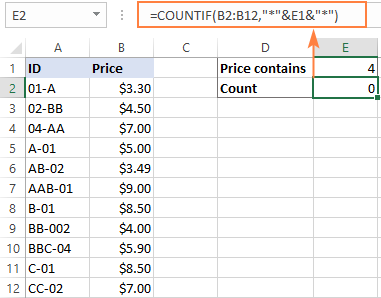

How to make wildcards work for numbers

The easiest solution is to convert numbers to text (for example, by using the Text to Columns feature) and then do a regular VLOOKUP, COUNTIF, MATCH, etc.

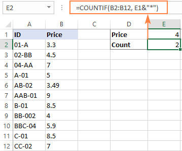
For instance, to get the count of cells that begin with the number in E1, the formula is:

=COUNTIF(B2:B12, E1&»*» )

In situation when this approach is not practically acceptable, you will have to work out your own formula for each specific case. Alas, a generic solution does not exist 🙁 Below, you will find a couple of examples.

Example 1. Excel wildcard formula for numbers

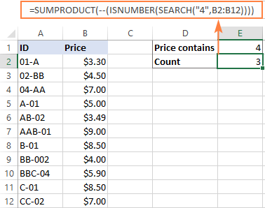
This example shows how to count numbers that contain a specific digit. In the sample table below, suppose you want to calculate how many numbers in the range B2:B12 contain «4». Here’s the formula to use:

=SUMPRODUCT(—(ISNUMBER(SEARCH(«4», B2:B12))))

How this formula works

Working from the inside out, here’s what the formula does:

The SEARCH function looks for the specified digit in every cell of the range and returns its position, a #VALUE error if not found. Its output is the following array:

The ISNUMBER function takes it from there and changes any number to TRUE and error to FALSE:

A double unary operator (—) coerces TRUE and FALSE to 1 and 0, respectively:

Finally, the SUMPRODUCT function adds up the 1’s and returns the count.

Note. When using a similar formula in your worksheets, in no case you should include «$» or any other currency symbol in the SEARCH function. Please remember that this is only a «visual» currency format applied to the cells, the underlying values are mere numbers.

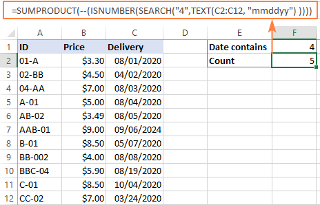
Example 2. Wildcard formula for dates

The SUMPRODUCT formula discussed above works beautifully for numbers but will fail for dates. Why? Because internally Excel stores dates as serial numbers, and the formula would process those numbers, not the dates displayed in cells.

To overcome this obstacle, utilize the TEXT function to convert dates to text strings, and then feed the strings to the SEARCH function.

Depending on exactly what you aim to count, the text formats may vary.

To count all the dates in C2:C12 that have «4» in the day, month or year, use «mmddyyyy»:

=SUMPRODUCT(—(ISNUMBER(SEARCH(«4»,TEXT(C2:C12, «mmddyyyy»)))))

To count only the days that contain «4» ignoring months and years, use the «dd» text format:

=SUMPRODUCT(—(ISNUMBER(SEARCH(«4»,TEXT(C2:C12, «dd»)))))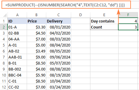

That’s how to use wildcards in Excel. I hope this information will prove useful in your work. Anyway, I thank you for reading and hope to see you on our blog next week!

Источник

Excel has 3 wildcards you can use in your formulas:

Asterisk (*) – zero or more characters.
Question mark (?) – any one character.
Tilde (~) – escape for literal character (~*) a literal question mark (~?), or a literal tilde (~~).

Contents

1 What is wildcard in Excel?
2 How do you use wildcard characters?
3 How do I use Asterisk in Excel?
4 How do I filter wildcards in Excel?
5 Why is my wildcard not working Excel?
6 How do I find and replace wildcard characters in Excel?
7 How do you use wildcards to search files and folders?
8 Can you use a wildcard in an Excel IF statement?
9 How do I filter special characters in Excel?
10 What does * mean in Excel formula?
11 How do you do a Vlookup with wildcards in Excel?
12 How do you use if and?
13 What are wildcards in Windows 10?
14 How many wild characters are present for searching files folder?
15 How do I search for an exact phrase in Windows 10?
16 How do I match a string in Excel?
17 How do you match a name in Excel where it is spelling different?
18 How do I write regex in Excel?
19 How do I get UTF 8 characters in Excel?
20 What is the use of * in Excel?

What is wildcard in Excel?

How do you use wildcard characters?

The CHARLIST is enclosed in brackets ([ ]) and can be used with wildcard characters for more specific matches.
Examples of wildcard character pattern matching in expressions.

C haracter(s)	Use to match
? or _ (underscore)	Any single character
* or %	Zero or more characters

How do I use Asterisk in Excel?

The tilde causes Excel to handle the next character literally. In this case we are using “~*” to match a literal asterisk, but this is surrounded by asterisks on either side, in order to match an asterisk anywhere in the cell. If you just want to match an asterisk at the end of a cell, use: “*~*” for the criteria.

How do I filter wildcards in Excel?

#1 Filter Data using Excel Wildcard Characters

Select the cells that you want to filter.
Go to Data –> Sort and Filter –> Filter (Keyboard Shortcut – Control + Shift + L).
Click on the filter icon in the header cell.
In the field (below the Text Filter option), type A*
Click OK.

Why is my wildcard not working Excel?

How do I find and replace wildcard characters in Excel?

Replacing a wildcard character

Press Ctrl + H to open the Find and Replace window.
Press Replace.
If we didn’t use tilde and asterisk (~*), just asterisk (*) the result would be like this.
Excel would treat asterisk as any number of characters (all the text in a cell) and convert it to a word in replace with.

How do you use wildcards to search files and folders?

Can you use a wildcard in an Excel IF statement?

How do I filter special characters in Excel?

Re: how to filter special characters in Excel
You can use ‘custom filter’ option available in filter option to find text with special characters. You just need to place ~ before the special character you want to filter.

What does * mean in Excel formula?

In Excel formula, the symbol “*” means multiplication. Say cell A1 contains 5 and cell A2 contains 8.

How do you do a Vlookup with wildcards in Excel?

How do you use if and?

When you combine each one of them with an IF statement, they read like this:

AND – =IF(AND(Something is True, Something else is True), Value if True, Value if False)
OR – =IF(OR(Something is True, Something else is True), Value if True, Value if False)
NOT – =IF(NOT(Something is True), Value if True, Value if False)

What are wildcards in Windows 10?

How many wild characters are present for searching files folder?

How do I search for an exact phrase in Windows 10?

How do I match a string in Excel?

Compare two strings

=A1=A2 // returns TRUE.
=EXACT(A1,A2) // returns FALSE.
=IF(EXACT(A2,A2),”Yes”,”No”)

How do you match a name in Excel where it is spelling different?

To match spelling different names, you can use the basic not equal sign ‘<>‘.

First, select the cell where you want to show the spelling differs names.
Here, I selected the H5 cell to place the result.
Now, you can write the formula in the formula bar or into your selected cell.
Type the formula. =B5<>E5.

How do I write regex in Excel?

The methods we can use are:

Test – check if the pattern can be found in the string. Returns True if it is found, False if it isn’t.
Execute – returns occurrences of the pattern matched against the string.
Replace – replaces occurrences of the pattern in the string.

How do I get UTF 8 characters in Excel?

View Unicode characters in Excel:

Open Excel from your menu or Desktop.
Navigate to Data → Get External Data → From Text.
Navigate to the location of the CSV file you want to import.
Choose the Delimited option.
Set the character encoding File Origin to 65001: Unicode (UTF-8) from the drop-down list.

What is the use of * in Excel?

Example

Data
Formula	Description
=PRODUCT(A2:A4)	Multiplies the numbers in cells A2 through A4.
=PRODUCT(A2:A4, 2)	Multiplies the numbers in cells A2 through A4, and then multiplies that result by 2.
=A2A3A4	Multiplies the numbers in cells A2 through A4 by using mathematical operators instead of the PRODUCT function.

Источник

How to Use Wildcards in Excel: Examples with VLOOKUP, COUNTIF, + more

Wildcards are some special characters that play the role of joker cards in Excel🃏

How? You can use them as a substitute for any character you are unsure about. By doing so, you can do so much in Microsoft Excel which would have been impossible (or at least very difficult) otherwise.

To learn all about using wildcard characters in Excel, continue reading the guide below.

And as you move forward, download our free sample Excel workbook here to practice side by side.

How to use wildcards in Excel

There are a total of three wildcard characters in Excel.

asterisk (*)
question mark (?)
tilde (~)

Each of these characters has a different use. You can use them to perform partial matches. Or as a comparison criterion to filter data or to find common values.

Let’s see how you can use each of these wildcard characters through the examples below.

The asterisk wildcard character

The first and the most dynamic of all, an asterisk is used as a substitute for any number of characters.

For example, if we use an asterisk with a word as (Ma*), it will represent all the strings that start with the two alphabets “Ma”. These could be Man, Matter, Match, and any word that starts with the alphabets “Ma”.

Time we see it working in Excel? Check the image below that has a list of fruits.

The data above contains a few fruit names that end with the letter ‘e’. Can we readily filter these out? Here’s how you can do it:

Select the column header of your dataset.
Go to Data > Sort & Filter > Filters.
Once you have the filters applied, click on the drop-down menu icon to launch the filter menu.
In the search bar, write the filter criteria as follows:

An asterisk with an “e” tells the Excel filter to show every value with an “e” at the end. Irrespective of the number of characters that come before “e”.

And here comes the magic of the asterisk. ✨

Excel filters out all the fruits that end in the letter “e”.

Pro Tip!

What you must notice is that each fruit has a different spelling.

The word “Orange” has five letters to its name before the letter “e”.
The word “Pineapple” has eight letters to its name before the letter “e”.
The word “Apple” has four letters to its name before the letter “e”.

But regardless of the number of characters before “e”, Excel filters all the words ending in “e”.

Pretty cool, right? 🤩 This was just one example of its use. An asterisk can be used in place of any character, in any position.

For example, from the same list of fruits, what if you want to filter out fruits beginning with the letter “A”?

To do so:

Launch the Filter Menu.
Define the filter criteria as:

Here, we need to filter out fruits starting with the letter “A”, irrespective of the number of characters in the name of the fruit after A.

So the criteria is an asterisk after A (a*).

Hit Enter and there you go.

All the words starting with the letter “a” are filtered out.

Pro Tip!

Wildcards can be used even when you are unsure about the letter case.

Like in the above example, we defined the criteria as (a*). Whereas, the fruits in the list above start with a capital A. The results, however, remain unchanged.

The question mark wildcard character

A question mark is used to substitute a single unknown character.

For example, here is a list of words (some of which start with the alphabet S and end in N).

From this list, can we filter out all the three-letter words that start with “s” and end with “n”?

To do so, we must replace the middle character of “S” and “N” with a question mark as shown below.

s?n

This tells Excel to filter out all the words that start with “S” and end with an “N” with any single character in between.

And here come the results.

Interesting, isn’t it?

And what if we want to filter out words that have two characters?

Simple – Type “??” in the filter box and Excel will filter out all two-letter words as shown below.

The tilde wildcard character

Until now, we have seen how helpful the above two wildcard characters are. But what if you want to use them as literal characters and not as wildcard characters?

This is where the tilde comes in. It allows us to use the asterisk as a literal asterisk or a question mark as a literal question mark.

See the tilde work in Excel below.

The data in the image above has words with asterisks, question marks, and tildes in them.

Let’s see what happens when we type a question mark in the filter box.

No matches? Huh.

Excel considered the question mark as a wildcard character. Doing so, it only looks for single-character words – and the data has none of them so you pull off nothing.

But what if we want Excel to filter the values ending with a literal question mark?

Let’s try using a tilde ‘~’ before the question mark.

In this search, the filter results contain all the words with a literal question mark.

Brain Teaser! What if you want to search for words that contain a literal tilde? The concept is still the same.

Kasper Langmann, Microsoft Office Specialist

In the filter criteria box, add another tilde to the tilde as shown below.

And you see the results. Excel finds the words containing a tilde.

So technically a tilde nullifies the effect of other wildcard characters. Funny, isn’t it? 😁

Using wildcards with Excel formulas

Till now, we have learned the general use of Excel wildcard characters.

But that’s not it. Wildcard characters are the most useful when used in pair with other functions of Excel.

Most importantly, the VLOOKUP, and COUNTIF functions. Time we see how to do so? Let’s dive into it.

How to use wildcards with VLOOKUP

Using the VLOOKUP function, you can search for a value from any dataset in Excel.

That’s true – but how can you use the VLOOKUP function when you are unsure about the value to be looked up?

Using the wildcard characters 🎯

The data in the image below has a list of locations – and for each of them, we want to find the number of umbrellas sold.

The number of umbrellas sold sits in another dataset (the lookup table) as shown below.

We want to match our entries in the ‘Location’ column with the ‘Location TXT’ column in the lookup table.

But here’s a problem – the lookup table has certain codes at the end of each location’s name.

Applying the VLOOKUP function using the names of locations only won’t yield us a thing. See for yourself.

We have set up the VLOOKUP formula that tells Excel to return the number of umbrellas sold in NewYork City from the lookup table.

= VLOOKUP (A2, A13:B18, 2, 0)

And guess what? Excel only returns the #N/A error. This is because the lookup table doesn’t contain simple locations but locations with codes.

To help this situation out, we need to perform a partial match. So, rewrite the VLOOKUP function as follows.

=VLOOKUP(A2&”*”, A13:B18, 2, 0)

Did you notice something different about the above function? The lookup value.

We added an ampersand (the concatenate function) next to our lookup value, followed by an asterisk.

So technically, we changed the lookup value from simple A2 (location name) to A2&* (location name and any number of characters after it).

Excel now looks for all values that have NewYork City, New York to them. Irrespective of what comes after this text string.

And Ta Da! Excel finds the number of umbrellas sold for NewYork City from the lookup table.

Turn the lookup table reference into an absolute reference. And drag and drop the results to all the locations.

Excel finds and returns the number of umbrellas sold for each location.

Even though we didn’t know the exact codes for each location, the asterisk replaced it and helped us extract the results based on a partial match. ✌

Pro Tip!

Do you know about the XLOOKUP function? It is the advanced version of the Excel VLOOKUP function.

The XLOOKUP function offers an in-built mode for performing wildcard character matches. And so, you don’t have to embed wildcard characters into the search criterion to perform a partial match as above. 💯

How to use wildcards with COUNTIF

Using wildcards with the COUNTIF function brings you a whole new level of ease.

Let’s see how through the example below.

Here comes a list of fruits. And this time, we want to count the fruits with seven characters in their name.

To do so, write the COUNTIF function as follows:

=COUNTIF(A2:A6,”???????”)

The above function tells Excel to find strings with any seven characters from the range A2:A6.

Counting Fruit Names with seven characters

Excel returns the count of 2. The above list has two fruits with seven characters to their name.

Which ones by the way? (Avocado🥑 and Apricot 🍊).

And what if we change the formula to,

=COUNTIF(A2:A7,”?*”)

This tells Excel to count the number of fruits (words) that have:

a single character (at least) and;
any number of characters (at most).

Counting Fruit Names with at least one character

Excel counts all the fruits as they all meet the criteria defined above.

Note that in the range of cells to be counted, we have also included a blank cell (cell A7). However, this cell is not counted by Excel as it doesn’t meet the defined criteria.

That’s it – Now what?

The guide above runs us through the smart use of Excel wildcard characters through practical examples. We also learned to use them together with two important Excel functions.

But that’s not it – there are several more ways how you can use wildcard characters in Excel. For example, with the find and replace feature of Excel. 💪

Some other functions of Excel where wildcard characters can come in handy include the SUMIF, IF, and VLOOKUP functions (advanced uses).

Need help figuring out where to start learning these functions? You’re just one click away from it. Click here to register for my free 30-minute email course to learn these and many more functions of Excel.

Kasper Langmann2023-02-23T15:24:41+00:00

Page load link

Источник

A wildcard is a special character that lets you perform «fuzzy» matching on text in your Excel formulas. For example, this formula:

=COUNTIF(B5:B11,"*combo")

counts all cells in the range B5:B11 that end with the text «combo». And this formula:

=COUNTIF(A1:A100,"???")

Counts all cells in A1:A100 that contain exactly 3 characters.

Available wildcards

Excel has 3 wildcards you can use in your formulas:

Asterisk (*) — zero or more characters
Question mark (?) — any one character
Tilde (~) — escape for literal character (~*) a literal question mark (~?), or a literal tilde (~~).

Note: wildcards only work with text, not numbers.

Example wildcard usage

Usage	Behavior	Will match
?	Any one character	«A», «B», «c», «z», etc.
??	Any two characters	«AA», «AZ», «zz», etc.
???	Any three characters	«Jet», «AAA», «ccc», etc.
*	Any characters	«apple», «APPLE», «A100», etc.
*th	Ends in «th»	«bath», «fourth», etc.
c*	Starts with «c»	«Cat», «CAB», «cindy», «candy», etc.
?*	At least one character	«a», «b», «ab», «ABCD», etc.
???-??	5 characters with hypen	«ABC-99″,»100-ZT», etc.
*~?	Ends in question mark	«Hello?», «Anybody home?», etc.
xyz	Contains «xyz»	«code is XYZ», «100-XYZ», «XyZ90», etc.

Wildcards only work with text. For numeric data, you can use logical operators.

More general information on formula criteria here.

Functions that support wildcards

Not all functions allow wildcards. Here is a list of the most common functions that do:

AVERAGEIF, AVERAGEIFS
COUNTIF, COUNTIFS
MAXIFS, MINIFS
SUMIF, SUMIFS
VLOOKUP, HLOOKUP
MATCH
SEARCH

Источник

Sometimes working with data is not that easy, sometimes we face complex problems.

Let’s say, you want to search for the text “Delhi” from the data. But, in that data, you have the word “New Delhi” not “Delhi”.

Now, in this situation, you can’t match or search. Here, you need a way that allows you to use only available value or partial value (Delhi) to match or search for the actual value (New Delhi). Excel Wildcard Characters are meant for this. These wildcard characters are all about searching/looking up a text with a partial match. In Excel, the biggest benefit of these characters is with lookup and text functions. It gives you more flexibility when the value is unknown or partially available. So today, in this post, I’d like to tell you what wildcard characters are, how to use them, their types, and examples to use them with different functions. So let’s get started.

What is Excel Wildcard Characters

Excel Wildcard Characters are special kinds of characters that represent one or more other characters. It’s used in regular expressions, by replacing them with unknown characters. In simple words, when you are not sure about an exact character to use, you can use a wildcard character in that place.

Types of Excel Wildcard Characters

In Excel, you have 3 different wildcard characters Asterisk, Question Mark, and Tilde. And each of these has its own significance and usage.

Ahead we’ll discuss each of these characters in detail so that you would be able to use them in different situations.

1. Asterisk(*)

An asterisk is one of the most popular wildcard characters.

It can find any number of characters (in sequence) from a text. For example, if you use Pi* it will give you words like Pivot, Picture, Picnic, etc.

If you notice, all these words have Pi in starting and then different characters after that. Let’s understand it’s working with an example.

Below you have data where you have names of cities and their classification in a single cell.

city data to use with asterisk wildcard characters in excel1

Now from here, you need to count the number of cities in each classification. and for this, you can use an asterisk with COUNTIF.

=COUNTIF(City,Classification&”*”)

formula to use with asterisk wildcard characters in excel

In this formula, you have combined classification text from the cell with an asterisk. So, the formula only matches the classification text in the cell and the asterisk works as the rest of the characters.

And in the end, you get the count of cities according to classification.

2. Question Mark

With a question mark, you can replace one single character from a text. In simple words, it helps you get more specific, still using a partial match. For example, if you use c?amps it will return champs and chimps from the data.

3. Tilde (~)

The real use of a tilde is to nullify the effect of a wildcard character. For example, let’s say you want to find the exact phrase pivot*. If you use pivot* as a string, it would give you any word that has champs at the beginning (such as pivot table, or pivot chart). To specifically the string pivot*, you need to use ~. So your string would be pivot~*. Here, ~ ensures that Excel reads the following character as is, and not as a wildcard.

Wildcard Characters with Excel Functions

We can easily use all three wildcard characters with all the top functions.

Functions like VLOOKUP, HLOOKUP, SUMIF, SUMIFS, COUNTIF, COUNTIFS, SEARCH, FIND, and INDEX MATCH.

You can extend this list with all the functions which you use for matching a value, for lookups, or finding a text.

Ahead, I’ll share with you some examples with functions + find and replace options + conditional formatting + with numbers.

1. With SUMIF

Below you have data where you have invoice numbers and their amount. And, we need to sum amounts where invoice numbers have “Product-A” in starting.

data to use wildcard characters with sumif excel

For doing this we can use SUMIF with wildcard characters. And the formula will be:

=SUMIF(F2:F11,”Product-A*”,G2:G11)

formula to use wildcard characters with sumif excel

In the above example, we have used an asterisk with the criteria at the end. As we have learned an asterisk can find a partial text with any number of sequence characters.

And, here we have used it with “Product-A”. So, it will match the values where “Product-A” is at the beginning of the value.

2. With VOOKUP

Let’s say you have a list of students with full name and their marks.

Now, you want to use VLOOKUP to get marks in another list in which you only have their first names.

And for this the formula will be:

=VLOOKUP(first_name&”*”,marks_table,2,0)

In the above example, you have used vlookup with an asterisk to get marks by only using the first name.

3. For Find and Replace

Using wildcard characters with find and replace option can do wonders for your data.

using excel wildcard characters with find replace options

In the above example, you have the word “ExcelChamps” which has different characters between it. And, you want to replace those characters with a simple space.

You can even do this by using replace option but in that case, you have to replace each character one by one.

But, you can use a question mark (?) to replace all the other characters with space. Find “Excel?Champs” & replace it with “Excel Champs” to remove all unwanted characters.

4. In Conditional Formatting

You can also use these wildcard characters with conditional formatting. Let’s say, from a list, you want to highlight the name of the cities which are starting with the letter A.

First of all, select the first entry from the list and then go to Home → Styles → Conditional Formatting.
Now, click on the “New Rule” option, and select use a formula to determine which cells to format”.
In the formula input box, enter =IF(COUNTIF(E2,”A*”),TRUE,FALSE).
Set the desired formatting, you want to use to highlight.

Now, I have used conditional formatting in the first cell of the list & I have to apply it to the entire list.
Select the first cell on which you have applied your formatting rule.
Go to Home → Clipboard → format painter.
Select the entire list and it will highlight all the names starting with the letter A.

5. Filter values

Wildcard characters work like magic in filters. Let’s say you have a list of cities, and you want to filter city names starting from A, B, C, or any other letter. You can use A* or B* or C* for that.

use excel wildcard characters with filters

This will give you the exact name of cities that are starting from that letter. And, if you want to search for any character which is ending with a specific letter you can use it before that letter (*A, *B,*C, etc.).

6. With Numbers

You can use these wildcards with numbers but you have to convert those numbers into text.

use wildcard characters in excel when you have only numbers

In the above example, you have used the match function and text function to perform a partial match. The text function returns an array by converting the entire range into the text and after that match function, lookup for a value which is starting from 98.

Sample File

Download this sample file from here to learn more.

Conclusion

With wildcard characters, you can enhance the power of functions when your data is not in a proper format.

These characters help you search or match a value using a partial match which gives you the power to deal with irregular text values. And the best part is you have three different characters to use.

Have you ever used these wildcard characters before?

Share your views with me in the comment section, I’d love to hear from you. And, don’t forget to share this tip with your friends.

Excel Formulas

More Formula

Excel 3D Reference
Hide Formula in Excel
R1C1 Reference Style in Excel

Источник

With wildcards in Excel, you can narrow down your search in spreadsheets. Here’s how to use these characters in filters, searches, and formulas.

Wildcard characters are special characters in Microsoft Excel that let you extend or narrow down your search query. You can use these wildcards to find or filter data, and you can also use them in formulas.

In Excel, there are three wildcards: Asterisk (*), question mark (?), and tilde (~). Each of these wildcards has a different function, and though only three, there’s a lot you can accomplish with them.

Wildcards in Excel

Asterisk *: Represent any number of characters where the asterisk is placed.
- A query such as *en will include both Women and Men, and anything else that ends in en.
- Ra* will include Raid, Rabbit, Race, and anything else starting with Ra.
- *mi* will include anything that has a mi in it. Such as Family, Minotaur, and Salami.
Question Mark ?: Represents any single character where the question mark is: S?nd. This includes Sand and Send. Moreover, ???? will include any 4 letter text.
Tilde ~: Indicates an upcoming wildcard character as text. For instance, if you want to search for a text that contains a literal asterisk and not a wildcard asterisk, you can use a tilde. Searching for Student~* will bring up only Student*, while searching for Student* will include every cell that starts with Student.

How to Filter Data With Wildcards in Excel

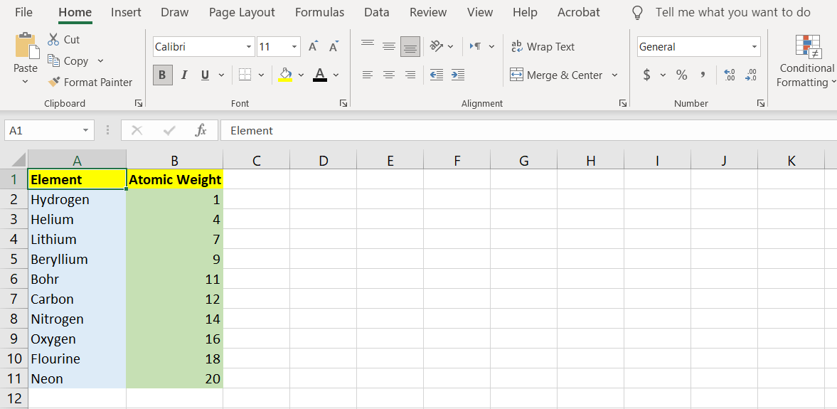
With wildcards, you can make a specific filter for your data in Excel. In this example spreadsheet, we have a list of the first ten elements from the periodic table. We’re going to make two different filters: First to get a list of elements that end with ium, and second to get a list of elements that only have four letters in their names.

Click the header cell (A1) and then drag the selection over to the last element (A11).
On your keyboard, press Ctrl + Shift + L. This will make a filter for that column.
Click the arrow next to the header cell to open the filter menu.
In the search box, enter *ium.
Press Enter.
Excel will now bring up all the elements in the list that end with ium.

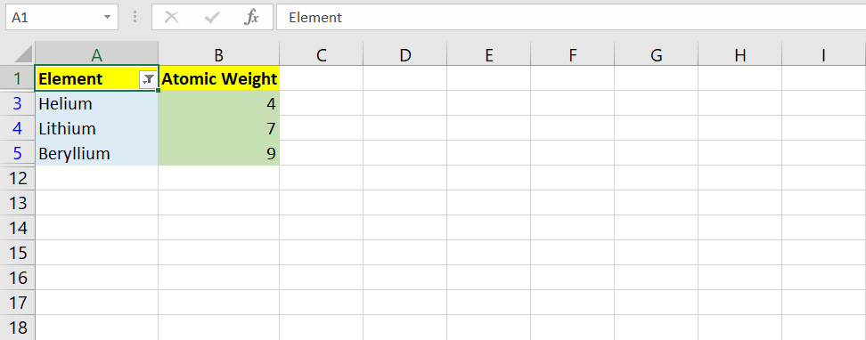
Now let’s run a filter to see which elements in this list have only four letters in their names. Since you’ve already created a filter, you’ll just need to adjust the content of the search box.

Click the arrow next to the header cell. This will open the filter menu.
In the search box, enter ????.
Press Enter.
Excel will now show only the elements that have four letters in their names.

To remove the filter and make all the cells visible:

Click the arrow next to header cell.
In the filter menu, under the search box, mark Select All.
Press Enter.

If you’re curious about the filter tool and want to learn more about it, you should read our article on how to filter in Excel to display the data you want.

How to Search Data With Wildcards in Excel

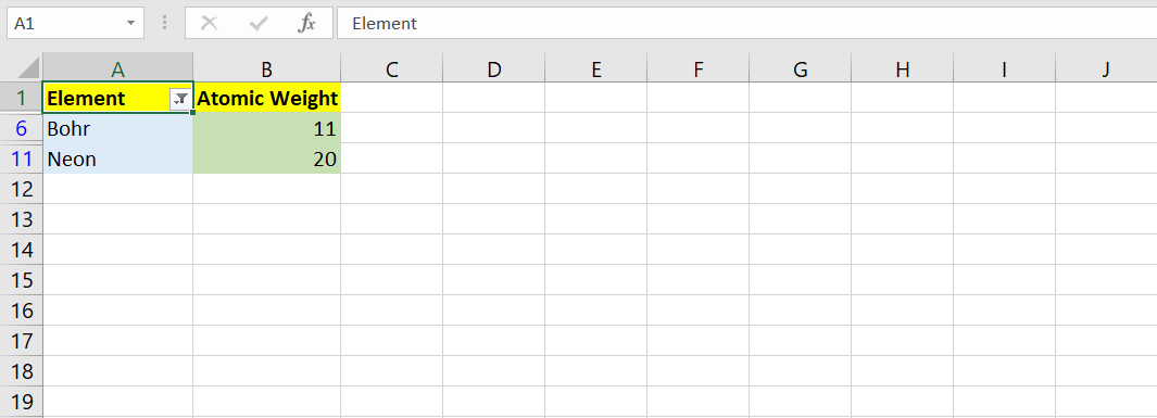
The Find and Replace tool in Excel supports wildcards and lets you use them to narrow down or expand your search. In the same spreadsheet, let’s try to search for elements that begin and end with N.

Press Ctrl + F on your keyboard to bring up the Find and Replace window.
In the text box in front of Find what enter N*N.
Click Find All.
The window will extend to display a list of cells that contain elements beginning and ending with N.

Now let’s run a more specific search. Which element in the list begins and ends with N, but has only four letters?

Press Ctrl + F on your keyboard.
In the text box, type N??N.
Click Find All.
The Find and Replace window will extend to show you the result.

How to Use Wildcards in Excel Formulas

While not all functions in Excel support wildcards, here are the six ones that do:

AVERAGEIF
COUNTIF
SUMIF
VLOOKUP
SEARCH
MATCH

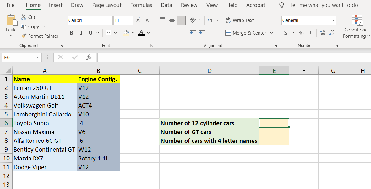
In this example, we have a list of cars and their engine configurations. We’re going to use the COUNTIF function to count three kinds of cars and then display the results in three separate cells. First, we can count how many cars are powered by 12-cylinder engines, then we can count how many cars have four-letter names.

Now that you have a grip on wildcards, it’s easy to guess that the first and second objectives can be accomplished solely with the asterisk.

Select cell E6 (in our example).
In the formula bar, enter the formula below:
```
=COUNTIF(B2:B11, "*12")
```
This formula will take the cells B2 to B11 and test them for the condition that the engine has 12 cylinders or not. Since this is regardless of the engine’s configuration, we need to include all the engines that end with 12, thus the asterisk.
Press Enter.
Excel will return the number of 12-cylinder cars in the list.

Counting the number of GT cars is done similarly. The only difference is an additional asterisk at the end of the name, which alerts us to any cars that do not end with GT but still contain the letter.

Select cell E7.
In the formula bar, enter the formula below:
```
=COUNTIF(A2:A11, "*GT*")
```
The formula will test cells A2 to A11 for the *GT* condition. This condition states that any cell that has the phrase GT in it, will be counted.
Press Enter.
Excel will return the number of GT cars.

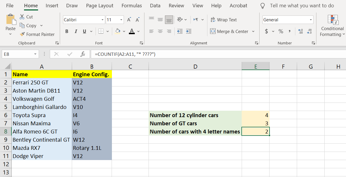
The final objective is slightly different. To count the cars that have four-letter model names, we’re going to need the question mark wildcard.

Select cell E8.
In the formula bar, enter the formula below:
```
=COUNTIF(A2:A11, "* ????")
```
This formula will test the car names, the asterisk states that the car brand can be anything, whereas the four question marks make sure that the car model is in four letters.
Press Enter.
Excel will return the number of cars that have four-letter models. In this case, it’s going to be the Golf and the DB11.

Get the Data You Want With Wildcards

Wildcards are simple in nature, yet they have the potential to help you achieve sophisticated things in Excel. Coupled with formulas, they can make finding and counting cells much easier. If you’re interested in searching your spreadsheet more efficiently, there are a couple of Excel functions that you should start learning and using.

Источник

Need more help?

Excel Wildcard Characters – An Introduction

#1 Filter Data using Excel Wildcard Characters

#2 Partial Lookup Using Wildcard Characters & VLOOKUP

3. Find and Replace Partial Matches

4. Count Non-blank Cells that Contain Text

Excel Wildcard Characters

Table of contents

Types

Type #1 – Asterisk (*)

Type #2 – Question Mark (?)

Type #3 – Tilde (~)

Examples

Example #1 – Usage of Excel Wildcard Character Asterisk (*)

Example #2 – Partial Lookup Value in VLOOKUP

Example #3 – Usage of Excel Wildcard Character Question Mark (?)

Recommended Articles

Excel wildcards

What are the wildcards in Excel?

How do you use wildcards in Excel?

Can I use wildcards in IF statements in Excel?

How do you use wildcards?

What are the 5 functions in Excel?

What is * in Excel formula?

Can you use wildcards in Vlookup?

How do I use a wildcard in VBA?

How do I use Countifs with wildcard characters?

How do you use wildcards in if function?

How if function works in Excel?

How do you do an if contains in Excel?

Wildcard

Available wildcards

Example wildcard usage

Functions that support wildcards

How To Use Wildcard In Excel?

What is wildcard in Excel?

How do you use wildcard characters?

How do I use Asterisk in Excel?

How do I filter wildcards in Excel?

Why is my wildcard not working Excel?

How do I find and replace wildcard characters in Excel?

How do you use wildcards to search files and folders?

Can you use a wildcard in an Excel IF statement?

How do I filter special characters in Excel?

What does * mean in Excel formula?

How do you do a Vlookup with wildcards in Excel?

How do you use if and?

What are wildcards in Windows 10?

How many wild characters are present for searching files folder?

How do I search for an exact phrase in Windows 10?

How do I match a string in Excel?

How do you match a name in Excel where it is spelling different?

How do I write regex in Excel?

How do I get UTF 8 characters in Excel?

Excel wildcard: find and replace, filter, use in formulas

Excel wildcard characters

Asterisk as a wildcard

Question mark as a wildcard

Tilde as a wildcard nullifier

Find and replace wildcards in Excel

How to search with wildcard

How to replace with wildcard

How to find and replace wildcard characters

Filter data with wildcards in Excel

Excel formulas with wildcard

Excel COUNTIF wildcard formula

Excel wildcard VLOOKUP formula

Excel wildcard for numbers

Find and Replace with wildcard number

Filter with wildcard number

Why Excel wildcard not working with numbers in formulas

How to make wildcards work for numbers

Example 1. Excel wildcard formula for numbers

Example 2. Wildcard formula for dates

What is wildcard in Excel?

How do you use wildcard characters?

How do I use Asterisk in Excel?

How do I filter wildcards in Excel?

Why is my wildcard not working Excel?

How do I find and replace wildcard characters in Excel?