
Where are my worksheet tabs?
Excel for Microsoft 365 Excel 2021 Excel 2019 Excel 2016 Excel 2013 Excel 2010 More…Less
If you can’t see the worksheet tabs at the bottom of your Excel workbook, browse the table below to find the potential cause and solution.
Note: The image in this article are from Excel 2016. Your view might be slightly different if you have a different version, but the functionality is the same (unless otherwise noted).
|
Cause |
Solution |
|---|---|
|
The window sizing is keeping the tabs hidden. |
If you still don’t see the tabs, click View > Arrange All > Tiled > OK. |
|
The Show sheet tabs setting is turned off. |
First ensure that the Show sheet tabs is enabled. To do this,
|
|
The horizontal scroll bar obscures the tabs. |
Hover the mouse pointer at the edge of the scrollbar until you see the double-headed arrow (see the figure). Click-and-drag the arrow to the right, until you see the complete tab name and any other tabs. |
|
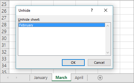
The worksheet itself is hidden. |
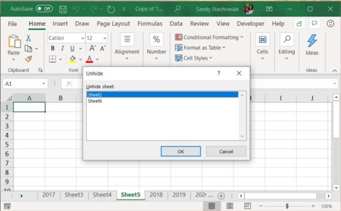
To unhide a worksheet, right-click on any visible tab and then click Unhide. In the Unhide dialog box, click the sheet you want to unhide and then click OK. |
Need more help?
You can always ask an expert in the Excel Tech Community or get support in the Answers community.
Need more help?
In Microsoft Excel, a sheet, sheet tab, or worksheet tab is used to display the worksheet that a user is currently editing. By clicking a worksheet tab (located at the bottom of the window), users may move between the various worksheets. Every Excel file may have multiple worksheets, but the default number is three.
Contents
- 1 Where is the sheet tab in Excel?
- 2 What are sheet tabs class 10th?
- 3 How do you add a sheet tab?
- 4 What is tab used for in Excel?
- 5 How do you tab in an Excel cell?
- 6 How do I view sheet tabs in Excel 2010?
- 7 What is sheet bar?
- 8 How do I create a new sheet in Class 10?
- 9 What do you mean by worksheet?
- 10 Why can’t I add a tab to my Excel spreadsheet?
- 11 How do I sort tabs in Google Sheets?
- 12 What are the 8 tabs in Excel?
- 13 What are the different tabs in Excel called?
- 14 What is the purpose of Tab key?
- 15 How do I get the tab name in Excel?
- 16 How do I activate the Tab key in Excel?
- 17 How do I view sheet tabs in Excel 2007?
- 18 How many sheets are in a workbook?
- 19 What is cell in Excel?
- 20 How do you copy worksheets?
Where is the sheet tab in Excel?
First ensure that the Show sheet tabs is enabled. To do this, For all other Excel versions, click File > Options > Advanced—in under Display options for this workbook—and then ensure that there is a check in the Show sheet tabs box.
What are sheet tabs class 10th?
Sheet tab is a part of Microsoft Excel, and it is the tab that is used for displaying the worksheet that is currently been edited by the user.
How do you add a sheet tab?
On the Home tab, in the Cells group, click Insert, and then click Insert Sheet. Tip: You can also right-click the selected sheet tabs, and then click Insert. On the General tab, click Worksheet, and then click OK.
What is tab used for in Excel?
It replaces the File Menu of earlier versions of Office and Excel. It is used to Open, Save, Print and Close files. The commands are organized by Tab and Group. At the highest level is the Ribbon for each Tab.
How do you tab in an Excel cell?
To tab text inside a table cell. Click or tap in front of the text or numbers you want to indent, and then press CTRL+TAB.
How do I view sheet tabs in Excel 2010?
How to Display Sheet Tabs in Excel 2010
- Open Excel.
- Click File.
- Choose Options.
- Select the Advanced tab.
- Check the box to the left of Show sheet tabs.
- Click OK.
a flat steel billet 4–22 mm thick and approximately 150–730 mm wide, produced by section and billet mills and in tended for hot-rolling into sheets 0.18–3.0 mm thick. It is used in the production of steel plate, dynamo and transformer steel, roofing iron, and steel sheet, as well as skelp for welded pipe.
How do I create a new sheet in Class 10?
Follow the given steps:
- Click on Insert –> Sheet option.
- Select the place where you want to insert the worksheet either before the current sheet or after the current sheet. or Click on empty space available in the sheet tab after last worksheet.
- Select the sheet options like New Sheet, No.
- Click on the OK button.
What do you mean by worksheet?
A Worksheet is a collection of cells organized in rows and columns. It is the working surface you interact with to enter data. Each worksheet contains 1048576 rows and 16384 columns and serves as a giant table that allows you to organize information.
Why can’t I add a tab to my Excel spreadsheet?
Can’t insert a new worksheet or delete an existing sheet? The option to add new sheet is greyed out? If the workbook structure is protected with a password, you’re unable to add, delete, move, copy, rename, hide or unhide any sheets. Here are 2 ways to unprotect workbook structure in Excel 2016 / 2013.
How do I sort tabs in Google Sheets?
To organize / reorder tabs in Google Sheets, simply click and drag the tabs to the location that you want them to be. Click near the name of the tab, hold the click, and then drag the cursor to the right or the left. Release your click when the tab is where you want it to be.
What are the 8 tabs in Excel?
Tabs. The tabs on the ribbon are: File, Home, Insert, Page layout, Formulas, Data, Review, View and Help.
What are the different tabs in Excel called?
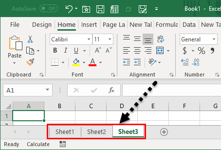
Click each of the three worksheet tabs—Sheet1, Sheet2 and Sheet3—to become familiar moving from sheet to sheet in the workbook.
What is the purpose of Tab key?
The tab key Tab ↹ (abbreviation of tabulator key or tabular key) on a keyboard is used to advance the cursor to the next tab stop.
How do I get the tab name in Excel?
Go to the cell which you want to reference the current sheet tab name, please enter =TabName() and then press the Enter key. Then the current sheet tab name will be display in the cell.
How do I activate the Tab key in Excel?
Tick “Select Locked Cells” in the protect sheet properties dialog. This will allow the tab key to access locked cells as desired. Tick “Select Locked Cells” in the protect sheet properties dialog. This will allow the tab key to access locked cells as desired.
How do I view sheet tabs in Excel 2007?
Excel 2007: Click the Office button, choose Excel Options, and then then enable the Show Sheet Tabs setting in the Display Options section of the Advanced options. Excel 2003 and earlier: Choose Tools, Options, Display, and then Show Sheet Tabs.
How many sheets are in a workbook?
By default, there are three sheets in a new workbook in all versions of Excel, though users can create as many as their computer memory allows. These three worksheets are named Sheet1, Sheet2, and Sheet3.
What is cell in Excel?
Cells are the boxes you see in the grid of an Excel worksheet, like this one. Each cell is identified on a worksheet by its reference, the column letter and row number that intersect at the cell’s location. This cell is in column D and row 5, so it is cell D5. The column always comes first in a cell reference.
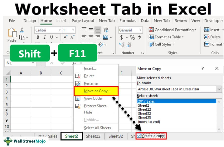
How do you copy worksheets?
Copy a worksheet in the same workbook
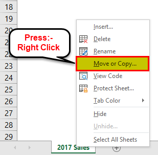
- Right click on the worksheet tab and select Move or Copy.
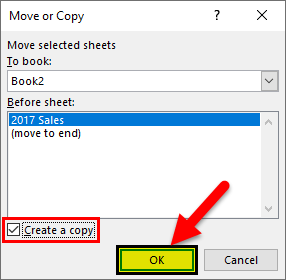
- Select the Create a copy checkbox.
- Under Before sheet, select where you want to place the copy.
- Select OK.
Содержание
- Where are my worksheet tabs?
- Need more help?
- Acquaintance with the Excel window and tabs panel
- The main window of the program
- Managing of the toolbar and bookmarks
- Excel Worksheet Tab
- Worksheet Tab in Excel
- #1 Change No. of Worksheets by Default Excel Creates
- #2 Create Replica of Current Worksheet
- #3 – Create Replica of Current Worksheet by Using Shortcut Key
- #4 – Create New Excel Worksheet
- #5 – Create New Excel Worksheet Tab Using Shortcut Key
- #6 – Go to the First Worksheet & Last Worksheet
- #7 – Move Between Worksheets
- #8 – Delete Worksheets
- #9 – View All the Worksheets
- Things to Remember
- Recommended Articles
Where are my worksheet tabs?
If you can’t see the worksheet tabs at the bottom of your Excel workbook, browse the table below to find the potential cause and solution.
Note: The image in this article are from Excel 2016. Your view might be slightly different if you have a different version, but the functionality is the same (unless otherwise noted).
The window sizing is keeping the tabs hidden.
If you restore multiple windows in Excel, ensure that the windows are not overlapping. Perhaps the top of an Excel window is covering the worksheet tabs of another window.
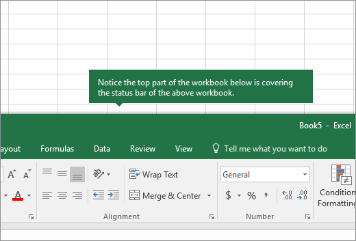
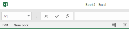
The status bar has been moved all the way up to the Formula Bar.
Tabs can also disappear if your computer screen resolution is higher than that of the person who last saved the workbook.
Try maximizing the window to reveal the tabs. Simply double-click the window title bar.
If you still don’t see the tabs, click View > Arrange All > Tiled > OK.
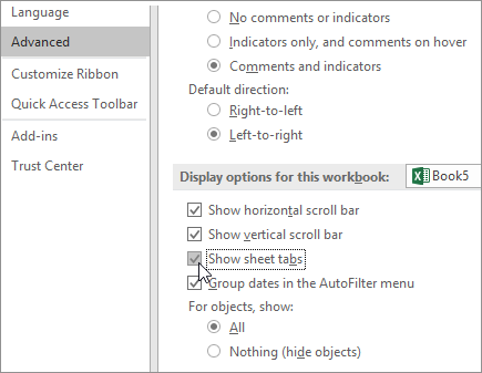
The Show sheet tabs setting is turned off.
First ensure that the Show sheet tabs is enabled. To do this,
For all other Excel versions, click File > Options > Advanced—in under Display options for this workbook—and then ensure that there is a check in the Show sheet tabs box.
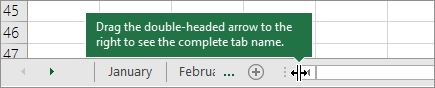
The horizontal scroll bar obscures the tabs.
Hover the mouse pointer at the edge of the scrollbar until you see the double-headed arrow (see the figure). Click-and-drag the arrow to the right, until you see the complete tab name and any other tabs.
The worksheet itself is hidden.
To unhide a worksheet, right-click on any visible tab and then click Unhide. In the Unhide dialog box, click the sheet you want to unhide and then click OK.
Need more help?
You can always ask an expert in the Excel Tech Community or get support in the Answers community.
Источник
Acquaintance with the Excel window and tabs panel
After downloading the Excel 2010 we will see the window (draw 1.1), that similar to the 2007 interface. It differs significantly from the older versions of 2003 and older. From this we can conclude – users of the 2007 version do not have to retrain much and get used to the new interface.
If you are just starting your first acquaintance with the program, you should not worry about what were its old versions: they are much inferior in terms of functionality and speed of the program.
The main window of the program
In the Excel window, a wide band with the tool buttons that are located on each tab is first of all thrown into the eye. In the interface of this version, the panel accounts for a large part of the program window. This often interferes with the viewing of large price lists. But the 2010 version allows by one mouse click to make a drop-down menu in Excel, which is very convenient.
The drawing 1. 1. This is the window after the program is downloaded:
The drawing 1. 2:
The toolbar is minimized.
The practical task 1. 1.
After downloading the program, take a closer look at the elements displayed in drawings 1. 1 and 1. 3. and try to make it so that the toolbar disappears into Excel, and then reappears again.
- Click the button as in the drawing 1. 1 to mineralize the tool bar (or press the keyboard shortcut CTRL + F1). This allows you to collapse the wide panel, as shown in the drawing 1. 2.
- Click on any tab, for example, «Home», as shown in the drawing 1. 2. For a while, all the bookmark tools will be available, covering the top of the page as in the drawing 1. 3.
Drawing 1. 3:
- Click anywhere outside of the panel, for example, on the sheet or the title of the window, to collapse the panel again.
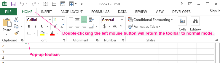
Double-click on any tab to make a pop-up menu in Excel.
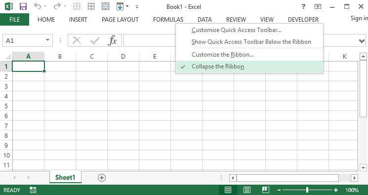
Call the context menu by right-clicking on the bookmark name and selecting the «Collapse ribbon» option. In this way, you fix the main taskbar in Excel and switch between the tool display modes.
As you can see, at first glance the interface version of 2010 is not much different from the 2007 version. But it has its own convenient and at first sight not noticeable advantages. In the process of active work with the program it is worthwhile to use by the various useful features to make the work comfortable.
The purpose of this lesson is to familiarize the user with the appearance of the program window, and also get acquainted with the basic tools and manage ones for comfortable work.
Источник
Excel Worksheet Tab


Worksheet Tab in Excel
The worksheet tabs in Excel are rectangular tabs visible on the bottom left of the Excel workbook. The “Activate” tab shows the active worksheet available to edit. By default, there can be three worksheet tabs opened. We can insert more tabs in the worksheet using the plus button provided at the end of the tabs. We can also rename or delete any of the worksheet tabs.
Worksheets are the platform for Excel software. In addition, these worksheets have separate tabs. Every Excel file must contain at least one worksheet in it. We have many more things with these worksheets tab in Excel.
We can find the worksheet tab at the bottom of every Excel worksheet tab.
In this article, we will take a complete tour of worksheet tabs regarding how to manage worksheets, rename, delete, hide, unhide, move or copy, the replica of the current worksheet, and many other things.
Table of contents
You are free to use this image on your website, templates, etc., Please provide us with an attribution link How to Provide Attribution? Article Link to be Hyperlinked
For eg:
Source: Excel Worksheet Tab (wallstreetmojo.com)
#1 Change No. of Worksheets by Default Excel Creates
You may have observed while opening the Excel file that it gives you three worksheets named “Sheet1,” “Sheet2,” and “Sheet3.”
We can modify this default setting and make our settings. Follow the below steps to change the settings.
- We must first go to the “FILE.”
Then, go to “OPTIONS.”
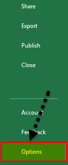
Under “GENERAL,” go-to “When creating new workbooks.”
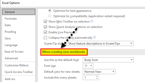
Under this, we must choose “Include this many sheets.”
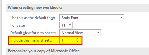
Here, we can modify how many worksheets tab in Excel must be included while creating a new workbook.

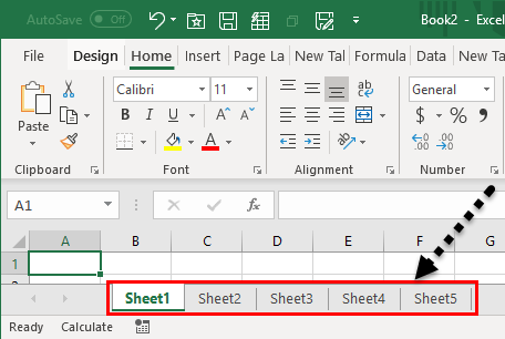
Click on “OK.” We will have a 5 Excel worksheets tab whenever we open a new workbook.
#2 Create Replica of Current Worksheet
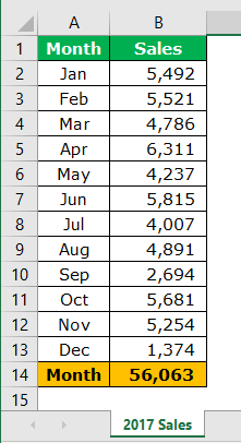
When you are working on an Excel file, you want to have a copy of the current worksheet at a certain point. For example, assume below is the worksheet tab you are working on at the moment.
- Step 1: First, we must right-click on the worksheet and select “Move or Copy.”
- Step 2: In the below window, click the checkbox “Create a copy.”
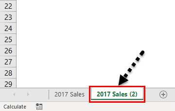
- Step 3: Click on “OK.” We will have a new sheet with the same data. The new worksheet name will be “2017 Sales (2).“
#3 – Create Replica of Current Worksheet by Using Shortcut Key
We can also create a replica of the current sheet by using this shortcut key.
- Step 1: We must select the sheet and hold the “Ctrl” key.
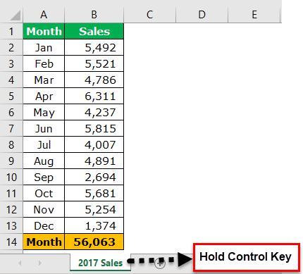
- Step 2: After holding the “Ctrl” key, hold the left button of the mouse key, and drag it to the right side. As a result, we would have a replica sheet now.
#4 – Create New Excel Worksheet
- Step 1: To create a new worksheet, we must click on the “plus” icon after the last worksheet.
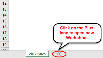
- Step 2: Once we click on the “PLUS” icon, we will have a new worksheet to the right of the current worksheet.

#5 – Create New Excel Worksheet Tab Using Shortcut Key
We can also create a new Excel worksheet tab using the shortcut key. For example, the shortcut key to insert the worksheet is “Shift + F11.”
If we press this key, it will insert the new worksheet tab to the left of the current worksheet.
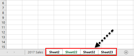
#6 – Go to the First Worksheet & Last Worksheet
Assume we are working with the workbook, which has many worksheets. Furthermore, we are moving between sheets regularly. Therefore, if we want to move to the last and first worksheets, we need to use the below technique.
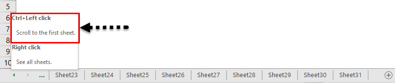
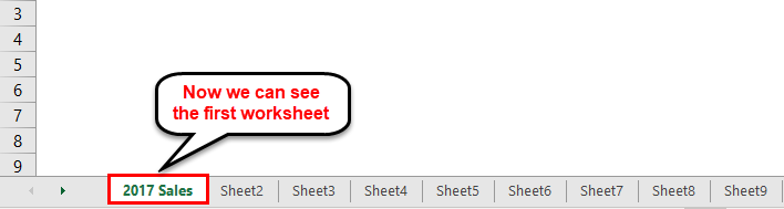
To come to the first worksheet, we must hold the “Ctrl” key and click on the arrow symbol to move to the first sheet.
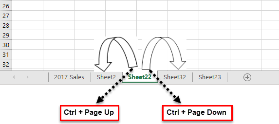
#7 – Move Between Worksheets
Going through all the worksheets in the workbook is a tough task if we move manually. So, we have shortcut keys to move between worksheets.
Ctrl + Page Up: This would go to the previous worksheet.
Ctrl + Page Down: This would go to the next worksheet.
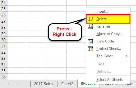
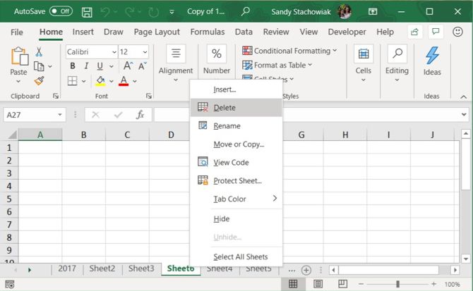
#8 – Delete Worksheets
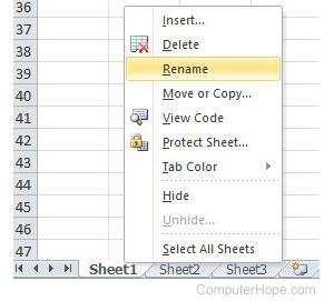
Like how we can insert new worksheets, we can delete the worksheet. To delete the worksheet, we must right-click on the required worksheet and click on “DELETE”.
If you want to delete multiple sheets simultaneously, we must hold the “Ctrl” key and select the sheets we want to delete.
Now, we can delete all the sheets at once.
We can also delete the sheet using the shortcut key, “ALT + E + L.”

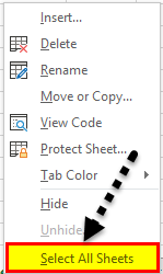
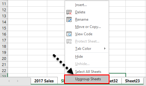
If we want to select all the sheets, we can right-click on any worksheets and choose “Select All Sheets.”
Once all the worksheets are selected, and if we want to unselect again, we must right-click on any worksheets and choose “Ungroup Worksheets.”
#9 – View All the Worksheets
If we have many worksheets and want to select a particular sheet, we do not know where exactly that sheet is.
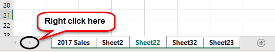
We can use the below technique to see all the worksheets. But, first, we must right-click on the move buttons at the bottom.
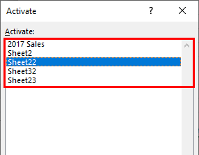
Consequently, we would see below the list of all the worksheets tab in the Excel file.
Things to Remember
- We can also hide and unhide sheets by right click on the sheetsUnhide Sheets By Right Click On The SheetsThere are different methods to Unhide Sheets in Excel as per the need to unhide all, all except one, multiple, or a particular worksheet. You can use Right Click, Excel Shortcut Key, or write a VBA code in Excel.read more .
- The shortcut key is “ALT + E + L.”
- For creating a replica sheet, the shortcut key is “ALT + E + M.”
- The shortcut key to select left side worksheets is “Ctrl + Page Up.”
- The shortcut key to select right side worksheets is “Ctrl + Page Down.”
Recommended Articles
This article has been guided to the Worksheet Tab in Excel. Here, we discuss how to manage worksheets, rename, delete, hide, unhide, move or copy and use shortcut keys with practical examples and a downloadable Excel template. You may learn more about Excel from the following articles: –
Источник
The worksheet tabs in Excel are rectangular tabs visible on the bottom left of the Excel workbook. The “Activate” tab shows the active worksheet available to edit. By default, there can be three worksheet tabs opened. We can insert more tabs in the worksheet using the plus button provided at the end of the tabs. We can also rename or delete any of the worksheet tabs.
Worksheets are the platform for Excel software. In addition, these worksheets have separate tabs. Every Excel file must contain at least one worksheet in it. We have many more things with these worksheets tab in Excel.
We can find the worksheet tab at the bottom of every Excel worksheet tab.
In this article, we will take a complete tour of worksheet tabs regarding how to manage worksheets, rename, delete, hide, unhide, move or copy, the replica of the current worksheet, and many other things.
Table of contents
- Worksheet Tab in Excel
- #1 Change No. of Worksheets by Default Excel Creates
- #2 Create Replica of Current Worksheet
- #3 – Create Replica of Current Worksheet by Using Shortcut Key
- #4 – Create New Excel Worksheet
- #5 – Create New Excel Worksheet Tab Using Shortcut Key
- #6 – Go to the First Worksheet & Last Worksheet
- #7 – Move Between Worksheets
- #8 – Delete Worksheets
- #9 – View All the Worksheets
- Things to Remember
- Recommended Articles
You are free to use this image on your website, templates, etc, Please provide us with an attribution linkArticle Link to be Hyperlinked
For eg:
Source: Excel Worksheet Tab (wallstreetmojo.com)
#1 Change No. of Worksheets by Default Excel Creates
You may have observed while opening the Excel file that it gives you three worksheets named “Sheet1,” “Sheet2,” and “Sheet3.”
We can modify this default setting and make our settings. Follow the below steps to change the settings.
- We must first go to the “FILE.”

- Then, go to “OPTIONS.”

- Under “GENERAL,” go-to “When creating new workbooks.”

- Under this, we must choose “Include this many sheets.”

- Here, we can modify how many worksheets tab in Excel must be included while creating a new workbook.

- Click on “OK.” We will have a 5 Excel worksheets tab whenever we open a new workbook.

#2 Create Replica of Current Worksheet
When you are working on an Excel file, you want to have a copy of the current worksheet at a certain point. For example, assume below is the worksheet tab you are working on at the moment.
- Step 1: First, we must right-click on the worksheet and select “Move or Copy.”
- Step 2: In the below window, click the checkbox “Create a copy.”
- Step 3: Click on “OK.” We will have a new sheet with the same data. The new worksheet name will be “2017 Sales (2).“
#3 – Create Replica of Current Worksheet by Using Shortcut Key
We can also create a replica of the current sheet by using this shortcut key.
- Step 1: We must select the sheet and hold the “Ctrl” key.
- Step 2: After holding the “Ctrl” key, hold the left button of the mouse key, and drag it to the right side. As a result, we would have a replica sheet now.
#4 – Create New Excel Worksheet
- Step 1: To create a new worksheet, we must click on the “plus” icon after the last worksheet.
- Step 2: Once we click on the “PLUS” icon, we will have a new worksheet to the right of the current worksheet.
#5 – Create New Excel Worksheet Tab Using Shortcut Key
We can also create a new Excel worksheet tab using the shortcut key. For example, the shortcut key to insert the worksheet is “Shift + F11.”
If we press this key, it will insert the new worksheet tab to the left of the current worksheet.
#6 – Go to the First Worksheet & Last Worksheet
Assume we are working with the workbook, which has many worksheets. Furthermore, we are moving between sheets regularly. Therefore, if we want to move to the last and first worksheets, we need to use the below technique.
To come to the first worksheet, we must hold the “Ctrl” key and click on the arrow symbol to move to the first sheet.
#7 – Move Between Worksheets
Going through all the worksheets in the workbook is a tough task if we move manually. So, we have shortcut keys to move between worksheets.
Ctrl + Page Up: This would go to the previous worksheet.
Ctrl + Page Down: This would go to the next worksheet.
#8 – Delete Worksheets
Like how we can insert new worksheets, we can delete the worksheet. To delete the worksheet, we must right-click on the required worksheet and click on “DELETE”.
If you want to delete multiple sheets simultaneously, we must hold the “Ctrl” key and select the sheets we want to delete.
Now, we can delete all the sheets at once.
We can also delete the sheet using the shortcut key, “ALT + E + L.”
If we want to select all the sheets, we can right-click on any worksheets and choose “Select All Sheets.”
Once all the worksheets are selected, and if we want to unselect again, we must right-click on any worksheets and choose “Ungroup Worksheets.”
#9 – View All the Worksheets
If we have many worksheets and want to select a particular sheet, we do not know where exactly that sheet is.
We can use the below technique to see all the worksheets. But, first, we must right-click on the move buttons at the bottom.
Consequently, we would see below the list of all the worksheets tab in the Excel file.
Things to Remember
- We can also hide and unhide sheets by right click on the sheetsThere are different methods to Unhide Sheets in Excel as per the need to unhide all, all except one, multiple, or a particular worksheet. You can use Right Click, Excel Shortcut Key, or write a VBA code in Excel. read more.
- The shortcut key is “ALT + E + L.”
- For creating a replica sheet, the shortcut key is “ALT + E + M.”
- The shortcut key to select left side worksheets is “Ctrl + Page Up.”
- The shortcut key to select right side worksheets is “Ctrl + Page Down.”
Recommended Articles
This article has been guided to the Worksheet Tab in Excel. Here, we discuss how to manage worksheets, rename, delete, hide, unhide, move or copy and use shortcut keys with practical examples and a downloadable Excel template. You may learn more about Excel from the following articles: –
- Insert Tab in Excel
- What is Accounting Worksheet?
- Excel VBA Worksheets
- Strikethrough in Excel
Updated: 04/01/2018 by
In Microsoft Excel, a sheet, sheet tab, or worksheet tab is used to display the worksheet that a user is currently editing. By clicking a worksheet tab (located at the bottom of the window), users may move between the various worksheets.
Every Excel file may have multiple worksheets, but the default number is three. These tabs are labeled «Sheet 1,» «Sheet 2,» and «Sheet 3.» Users may add, move, and rename worksheets. Instructions on how to perform these operations are linked in the related pages section below.
Tip
Use the shortcut key Alt+Shift+F1 to insert a new sheet while in Excel.
Sheet, Software terms, Spreadsheet terms, Tab, Worksheet
The ribbon, tabs, commands gridlines, control buttons, etc. that a user can see and interact with on the screen after opening an Excel spreadsheet are called User Interface Environment in MS Excel.
Excel is an electronic spreadsheet program, developed by Microsoft Corporation. An Excel Spreadsheet is used to record, validate and analyze the numeric data for maintaining Payrolls, Selling and purchasing product orders, Progress Reports, family budgets, and more.
These are calculated whether using general, financial, logical, statistical, engineering or other functions and formulas. The features in the excel environment are explained below in the screenshot.

Table of Contents
- User Interface to MS Excel
- Quick Access Toolbar:
- File Menu:
- Tell me:
- Title Bar:
- Sign in:
- Share:
- Control Buttons:
- Ribbon:
- Ribbon Display Options:
- Tabs:
- Groups:
- Commands
- Name Box:
- Insert Functions:
- Formula bar:
- Row and Column Headings:
- Vertical/Horizontal Scrollbar:
- Page View Options:
- Zoom Slider/Toolbar:
- Click to Select All:
- Gridlines:
- Cell in Excel:
- Cell Address:
- Active Cell:
- Active Sheet/sheet tab:
- Range of cells:
- Sheet tabs:
- Insert New Worksheet:
Quick Access Toolbar:
The Quick Access Toolbar appears at the top left corner of the Excel application and other MS Office suites. The default commands of the Quick Access Toolbar are Save, Undo and Redo.
In the graphical user interface environment in MS Excel, the File menu is also known as the File Tab, used to control and access the file functions of the MS Office suite.
Officially, it handles files using the file menu commands such as new, open, save, save, print, share, export, publish, close, account and options. To read the File menu features in an Excel environment click here.
Tell me:
In the user interface of Microsoft Excel, the tell me to search box helps you search the command quickly and easily without going to the ribbon tab or group. Here you can type any command name you want to use or apply to the Sheet/Document.
Title Bar:
You can see the title bar at the top of the excel spreadsheet application (MS Office suites) with the name currently being used. The name of the workbook appears in the middle of the title bar. The name of the workbook here we called is a title.
Sign in:
Microsoft’s free account is used to purchase, activate, and access Microsoft services. You can save and receive your documents from anywhere using the service. You can also use this account to use and access OneDrive, Skype, and Microsoft store.
This option appears at the top right corner, underneath the close button, you can save your work on different platforms by sharing with caring. These Platforms are Google Cloud, One Drive, E-mail, Blogs, people, etc.
Control Buttons:
The Minimize, Restore Down/Maximize and Close buttons are called Control Buttons. These appear at the top right corner of the (MS Office Suite of Applications) Excel Spreadsheet.
Ribbon:

The Ribbon is a collection of groups, commands and functions and locates under each Tab such as Home, Insert, Design, Layout, References, Mailings, Review and View, It is designed to help you quickly and easily find the groups and commands to complete a task you want.
Ribbon Display Options:

The Ribbon Display options are located at the right corner of the title bar and the 4th position on the left of the Control buttons. The Ribbon Display Options include Auto-Hide Ribbon, Show Tabs, Show Tabs and Commands.
Tabs:

Home, Insert, Page Layout, Formulas, Data, Review, and view are called Tabs. Each tab is a form of group. Similarly, each Group is a form of the command.
Groups:

Each tab is a form of group. Similarly, each group is a form of the command. For example, Groups on the Home tab include Clipboard, Font, Alignment, Number, Style, Cells, and Editing.
Commands

A command is part of a group. And access to a specific piece of work. For example, the Font group commands include bold, italic, underline, etc.
Name Box:
It is the reference (address) for a specific cell or range of cells or you can set the name for a particular cell or range of cells in an excel spreadsheet.
Insert Functions:
It helps to get the result by using a particular function based on its arguments. This is one of the features of Excel.
Formula bar:
In the Formula bar, you can view and modify the function or formula that applies to any cell in the sheet for any calculation.
Row and Column Headings:
The column is a collection of Vertical light grey coloured lines containing the letters used to identify each column in a worksheet.
The column heading appears on the top of it (above the first row). The row is a collection of Horizontal light grey coloured lines containing the number used to identify each row in a worksheet. The Row Heading appears at the beginning of it (left of the first column).
Without Row and Column Headings in excel you cannot perform an autofill feature.
Vertical/Horizontal Scrollbar:
The scrollbar is used to view the worksheet in any part by using the Vertical or Horizontal scrollbar whether by moving up, down, left or right.
Page View Options:
Page View Options appear at the right but one on the taskbar. These are
Normal: Normal is a default view and is easier to work in this mode in the worksheet.
Page Layout: In the Page Layout mode, the worksheet is divided into more page sizes for print preview.
Page Break Preview: The Page Break Preview shows the worksheet as separate pages where there are the contents to see how a page look likes.
Zoom Slider/Toolbar:
To zoom in and out excel spreadsheet in the desired size, use the Zoom slider, which appears at the bottom right corner of the workbook.
Click to Select All:
Click on the top left of the common area (Under the Name Box) of the Column and Row Headings to select the entire worksheet. Just like Ctrl + A.
Gridlines:
The Gridlines are the collection of Horizontal and Vertical light grey coloured lines in a worksheet.
Cell in Excel:
In the Microsoft Excel Spreadsheet Environment, A cell is an Intersection of Rows and columns to form like a rectangle in a worksheet.
Cell Address:
The location of a cell is identified by its column letter and the row number is called, cell address or cell reference.
Active Cell:
An Active Cell in the graphical user interface is where it is bold with a dark outline. An Active cell is an identifiable mark that can be accepted to enter and edit the content.
Active Sheet/sheet tab:
For a selected worksheet that is currently being used, the name of the sheet tab is in bold and appears at the bottom left corner of the workbook.
Range of cells:
In the Microsoft Excel Spreadsheet Environment, More than two cells that are selected horizontally or vertically are called a range of cells.
Sheet tabs:
In the user interface environment in MS Excel, The name of the sheets that appears from the bottom left corner of the worksheet are called sheet tabs.
Insert New Worksheet:
To insert more worksheets in a workbook, click the insert sheet tab button, located right to the sheet tabs.
-
What is an Active cell in Excel?
An Active Cell is where it is bold with a dark outline. An Active cell is an identifiable mark that can be accepted to enter and edit the content.
-
What is an active Sheet?
For a selected worksheet that is currently being used, the name of the sheet tab is in bold and appears at the bottom left corner of the workbook.
-
What is the range of cells in excel?
In the Microsoft Excel Spreadsheet Environment, More than two cells that are selected horizontally or vertically are called a range of cells.
-
What is the sheet tab in excel?
In the Microsoft Excel Spreadsheet Environment, The name of the sheets that appears from the bottom left corner of the worksheet is called sheet tabs.
-
What is a cell Address in Excel?
The location of a cell is identified by its column letter and the row number is called, cell address or cell reference.
-
What are Gridlines in Excel?
The Gridlines are the collection of Horizontal and Vertical light grey-coloured lines in a worksheet.
-
What is Formula Bar in Excel?
In the Formula bar, you can view and modify the function or formula that applies to any cell in the sheet for any calculation.
-
What is Insert Function in Excel?
It helps to get the result by using a particular function based on its arguments. This is one of the features in excel.
-
What is Name Box in Microsoft Excel?
If you can see the reference (address) for a specific cell or range of cells or you can set the name for a particular cell or range of cells in an excel spreadsheet.
In this article, we will learn about Excel Ribbons or Excel Tabs?
Scenario:
Once you open the excel software from the program menu, the first thing that you would notice is a large screen displayed. Since this is your first workbook, you will not notice any recently opened workbooks. There are various options that you can choose from; however, this being your first tutorial, I want you to open the Blank Workbook Once you click on the Blank workbook, you will notice the Blank Workbook opens up in the default format.
What are Ribbons in Excel
Ribbons are designed to help you quickly find the command that you want to execute in Excel 2016. Ribbons are divided into logical groups called Tabs, and Each tab has its own set of unique functions to perform. There are various tabs – Home, Insert, Page Layout, Formulas, Date, Review, and View.
How to Collapse (Minimize) Ribbons
If you do not want to see the commands in the Ribbons, you can always Collapse or Minimize Ribbons. For this RIGHT-click on Ribbon Area, and you will see various options available here. Here you need to choose “Collapse the Ribbon.” Once you choose this, the visible groups go away, and they are now hidden under the tab. You can always click on the tab to show the commands.
How to Customize Ribbons
Many times it is handy to customize Ribbons containing the commands that you frequently use. This helps save a lot of time and effort while navigating the excel workbook. In order to customize Excel Ribbons, RIGHT click on the Ribbon area and choose, customize the Ribbon
Once the dialog box opens up, click on the New Tab. Rename the New Tab and the New Group as per your liking. You can select the list of commands that you want to include in this new tab from the left-hand side. Once done, you will notice your customized tab appears in the Ribbon along with the other tabs.
What is Quick Access Toolbar
Quick Access Toolbar is a universal toolbar that is always visible and is not dependent on the tab that you are working with. For example, if you are in the Home Tab, you will see commands not only related to Home Tab but also the Quick Access Toolbar on the top executing these commands easily. Likewise, if you are in any other tab, say “Insert,” then again, you will have the same Quick Access Toolbar.
How to Customize Quick Access Toolbar
In order to customize the Quick Access Toolbar, RIGHT click on any part of the Ribbon and you will see the following. Once you click on Customize Quick Access Toolbar, you get the dialog box from where you can select the set of commands you want to see in the Quick Access Toolbar. The new quick access toolbar now contains the newly added commands. So as you can see, this is pretty simple.
What are the Tabs?
Tabs are nothing but various options available on the Ribbon. These can be used for easy navigation of commands that you desire to use.
Home Tab
Clipboard – This Clipboard Group is primarily used for Cut copy and paste. This means that if you want to transfer data from one place to another, you have two choices, either COPY (preserves the data in the original location) or CUT (deletes the data from the original location). Also, there are options of Paste Special, which implies copy in the desired format. We will discuss the details of these later in the Excel tutorials. There is also Format Painter Excel, which is used to copy the format from the original cell location to the destination cell location.
Fonts – This font group within the Home tab is used for choosing the desired Font and size. There are hundreds of fonts available in the dropdown which we can use for. In addition, you can change the font size from small to large, depending on your requirements. Also helpful is the feature of Bold (B), Italics (I), and Underline (U) of the fonts.
Alignment – As the name suggests, this group is used for alignment of tabs – Top, Middle, or Bottom alignment of text within the cell. Also, there are other standard alignment options like Left, middle, and right alignment. There is also an orientation option that can be used to place the text vertically or diagonally. Merge and Center can be used to combine more than one cell and place its content in the middle. This is a great feature to use for table formatting etc. Wrap text can be used when there is a lot of content in the cell, and we want to make all the text visible.
Number – This group provides options for displaying number format. There are various formats available – General, accounting, percentage, comma style in excel, etc. You can also increase and decrease the decimals using this group.
Styles – This is an interesting addition to Excel. You can have various styles for cells – Good, Bad, and Neutral. There are other sets of styles available for Data and Models like Calculation, Check, Warning, etc. In addition, you can make use of different Titles and Heading options available within Styles. The format Table allows you to quickly convert the mundane data into the aesthetically pleasing data table. Conditional formatting is used to format cells based on certain predefined conditions. These are very helpful in spotting the patterns across an excel sheet.
Cells – This group is used to modify the cell – its height and width etc. Also, you can hide and protect the cell using Format Feature. You can also insert and delete new cells and rows from this group.
Editing – This group within the Home Tab is useful for Editing the data on an excel sheet. The most prominent of the commands here is the Find and Replace in Excel Command. Also, you can use the sort feature to analyze your data – sort from A to Z or Z to A, or you can do a custom sort here.
Insert Tab
Tables – This group provides a superior way to organize the data. You can use Table to sort, filter, and format the data within the sheet. In addition, you can also use Pivot Tables to analyze complex data very easily. We will be using Pivot Tables in our later tutorials.
Illustrations – This group provides a way to insert pictures, shapes, or artwork into excel. You can insert the pictures either directly from the computer, or you can also use Online Picture Option to search for relevant pictures. In addition, shapes provide additional ready-made square, circle, arrow kind of shapes that can be used in excel. SmartArt provides an awesome graphical representation to visually communicate data in the form of List, organizational charts, Venn diagram to process diagrams. Screenshot can be used to quickly insert a screenshot of any program that is open on the computer.
Apps – You can use this group to insert an existing App into excel. You can also purchase an App from the Store section. Bing Maps app allows you to use the location data from a given column and plot it on Bing Maps. Also, there is a new feature called People Data, which allows you to transform boring data into an exciting one.
Charts – This is one of the most useful features in Excel
It helps you visualize the data in a graphical format. Recommended charts allow Excel to come up with the best possible graphical combination. In addition, you can make graphs on your own, and excel provides various options like Pie-chart, Line Chart, Column Chart in Excel, Bubble Chart k in Excel, combo chart in excel, Radar Chart in Excel, and Pivot Charts in Excel.
Sparklines – Sparklines are cute tiny charts that are made on the number of data and can be displayed with these cells. There are different options available for sparklines like Line Sparkline, Column Sparkline, and Win/Loss Sparkline. We will discuss this in detail in later posts.
Filters – There are two types of filters available – Slicer allows you to filter the data visually and can be used to filter tables, pivot tables data, etc. The Timeline filter allows you to filter the dates interactively.
Hyperlink – This is a great tool to provide hyperlinks from the excel sheet to an external URL or files. Hyperlinks can also be used to create a navigation structure with the excel sheet that is easy to use.
Text – This group is used to text in the desired format. For example, if you want to have the header and footer, you can use this group. In addition, WordArt allows you to use different styling for text. You can also create your signature using the Signature line feature.
Symbols – This primarily consists of two parts. First is Equation – this allows you to write mathematical equations that we cannot ordinarily write in an Excel sheet. Second is Symbols are special character or symbols that we may want to insert in the excel sheet for better representation
Page Layout Tab
Themes – Themes allow you to change the style and visual look of excel. You can choose various styles available from the menu. You can also customize the colors, fonts, and effects in the excel workbook.
Page Setup – This is an important group primarily used along with printing an excel sheet. You can choose margins for the print. In addition, you can choose your printing orientation from Portrait to Landscape. Also, you can choose the size of paper like A3, A4, Letterhead, etc. The print area allows you to see the print area within the excel sheet and is helpful in making the necessary adjustments. We can also add a break where we want the next page to begin in the printed copy. Also, you can add a background to the worksheet to create a style. Print Titles are like a header and footer in excel that we want to be repeated on each printed copy of the excel sheet.
Scale to Fit – This option is used to stretch or shrink the printout of the page to a percentage of the original size. You can also shrink the width as well as height to fit in a certain number of pages.
Sheet Options – Sheet options is another useful feature for printing. If we want to print the grid, then we can check the print gridlines option. If we want to print the Row and column numbers in the excel sheet, we can also do the same using this feature.
Arrange – Here, we have different options for objects inserted in Excel like Bringforward, Send Backward, Selection Pane, Align, Group Objects, and Rotate.
Formulas Tab
Function Library – This is a very useful group containing all the formulas that one uses in excel. This group is subdivided into important functions like Financial Functions, Logical Functions, Date & Timing, Lookup & References, Maths and Trigonometry, and other functions. One can also make use of Insert Function capabilities to insert the function in a cell.
Defined Names – This feature is a fairly advanced but useful feature. It can be used to name the cell, and these named cells can be called from any part of the worksheet without working about its exact locations.
Formula Auditing – This feature is used for auditing the flow of formulas and its linkages. It can trace the precedents (origin of data set) and can also show which dataset is dependent on this. Show formula can also be used to debug errors in the formula. The Watch window in excel is also a useful function to keep a tab on their values as you update other formulas and datasets in the excel sheet.
Calculations – By default, the option selected for calculation is automatic. However, one can also change this option to manual.
Data Tab
Get External Data – This option is used to import external data from various sources like Access, Web, Text, SQL Server, XML, etc.
Power Query – This is an advanced feature and is used to combine data from multiple sources and present it in the desired format.
Connections – This feature is used to refresh the excel sheet when the data in the current excel sheet is coming from outside sources. You can also display the external links as well as edit those links from this feature.
Sort & Filter – This feature can be used to sort the data from AtoZ or Z to Z, and also you can filter the data using the drop-down menus. Also, one can choose advanced features to filter using complex criteria.
Data Tools – This is another group that is very useful for advanced excel users. One can create various scenario analyses using What If analysis – Data Tables, Goal Seek in Excel, and Scenario Manager. Also, one can convert Text to Column, remove duplicates and consolidate from this group.
Forecast – This Forecast function can be used to predict the values-based on historical values.
Outline – One can easily present the data in an intuitive format using the Group and Ungroup options from this.
Review Tab
Proofing – Proofing is an interesting feature in Excel that allows you to run spell checks in the excel. In addition to spell checks, one can also make use of thesaurus if you find the right word. There is also a research button that helps you navigate the encyclopedia, dictionaries, etc. to perform tasks better.
Language – If you need to translate your excel sheet from English to any other language, then you can use this feature.
Comments – Comments are very helpful when you want to write an additional note for important cells. This helps the user understand clearly the reasons behind your calculations etc.
Changes – If you want to keep track of the changes that are made, then one can use the Track Changes option here. Also, you can protect the worksheet or the workbook using a password from this option.
View Tab
Workbook Views – You can choose the viewing option of the excel sheet from this group. You can view the excel sheet in the default normal view, or you can choose Page Break view, Page Layout view, or any other custom view of your choice.
Show – This feature can be used to show or not show Formula bars, grid lines, or Heading in the excel sheet.
zoom – Sometimes, an excel sheet may contain a lot of data, and you may want to change zoom in or zoom out desired areas of the excel sheet.
Window – The new window is a helpful feature that allows the user to open the second window and work on both at the same time. Also, freeze panes are another useful feature that allows freezing of particular rows and columns such that they are always visible even when one scrolls to the extreme positions. You can also split the worksheet into two parts for separate navigation.
Macros – This is again a fairly advanced feature, and you can use this feature to automate certain tasks in Excel Sheets. Macros are nothing but a recorder of actions taken in excel, and it has the capability to execute the same actions again if required.
Hope this article about What are Excel Ribbon or Excel Tabs? is explanatory. Find more articles on calculating values and related Excel formulas here. If you liked our blogs, share them with your friends on Facebook. And also you can follow us on Twitter and Facebook. We would love to hear from you, do let us know how we can improve, complement or innovate our work and make it better for you. Write to us at info@exceltip.com.
Popular Articles :
50 Excel Shortcuts to Increase Your Productivity : Get faster at your tasks in Excel. These shortcuts will help you increase your work efficiency in Excel.
How to use the VLOOKUP Function in Excel : This is one of the most used and popular functions of excel that is used to lookup value from different ranges and sheets.
How to use the IF Function in Excel : The IF statement in Excel checks the condition and returns a specific value if the condition is TRUE or returns another specific value if FALSE.
How to use the SUMIF Function in Excel : This is another dashboard essential function. This helps you sum up values on specific conditions.
How to use the COUNTIF Function in Excel : Count values with conditions using this amazing function. You don’t need to filter your data to count specific values. Countif function is essential to prepare your dashboard.
When you first start using Excel the screen can be a little overwhelming.
Once you have an understanding of each of the components you can quickly locate and use them with confidence.
Identifying the screen components
In the example below each of the screen component names are introduced.
The functionality of each component is detailed below.
Quick Access toolbar
The Quick Access toolbar (QAT) by default displays buttons for Save, Undo and Redo. However you can customise the toolbar to suit your needs by clicking the arrows at the end of the toolbar and add your own buttons or by right-clicking any button on any tab and selecting Add to Quick Access toolbar. To remove a button from your QAT toolbar just right-click it and select Remove from Quick Access toolbar.
Tabs
Command buttons are organised into tabs. For example, the commands that are used for saving, printing and sharing files are all located on the File tab. The Home tab houses the most commonly used command buttons for modifying and formatting your worksheet.
Ribbon
The Ribbon is the area on each tab that houses all of the command buttons. You may not need all of the commands on a Ribbon. You will come to find that you use only what you need. And if you like you can add these to the QAT toolbar too.
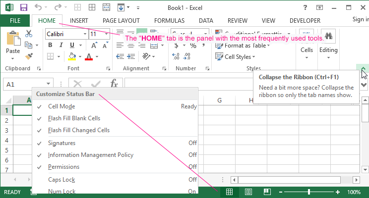
Tip: if you find you just aren’t getting enough screen space follow the steps below to hide the Ribbon and gain more screen area.
- Double-click the active tab name. The Ribbon will be hidden. Now click any tab once and the Ribbon will drop-down. When you click away the Ribbon will once again be hidden.
- In Office 2013 and 2016 you can click the Ribbon Display Options button on the top right of the screen. From here select the option that will best suit.
- If you are using a touch screen, from the Quick Access Toolbar try clicking the Touch/Mouse mode button. If you are using a mouse be sure to select this mode and you will suddenly have a more compact screen.
Note: to display the Ribbon again just double-click any tab.
Column headings, row numbers and cell addresses
The Column header bar identifies each column with a letter of the alphabet. Down the left side of the screen is the Row number bar, which identifies each row with a number. The intersection of a column and a row is known as a cell. For example, row 1 in column A is known as cell A1. Row 3 in column B is known as cell B3. And so on.
Cell selector
The cell selector is the heavy outlined rectangle that indicates the current working position. The cell pointer can be moved by clicking a cell with the left mouse button or by using the arrow keys. The cell pointer can be extended to cover multiple cells by clicking and dragging the mouse pointer across the selection. You will notice the row number and column letter “light up” to indicate the current position of the cell pointer. To learn more about selecting cells see my post Selecting cells and moving around an Excel worksheet.
Formula bar
The formula bar displays the content of the selected cell. If the cell holds a calculation the formula bar will show the formula while the actual cell in the grid area will show the result. You can click into the formula bar to update the cell content.
Sheet tabs
Sheet tabs (a.k.a. worksheets) are used to organise and categorise your data. For example, you could have individual worksheets for each month of the year, or each employee. When you create a new workbook (file) in Excel 2007 and 2010 you will be given Sheet 1, Sheet 2 and Sheet 3. However in Excel 2013 and 2016 you will be given just the one worksheet. You can easily add to these by clicking the Insert worksheet button.
Inserting a new worksheet in Excel 2013 or 2016
Inserting a new worksheet in Excel 2010
To rename the worksheet tab right-click the tab and then select Rename. Type the new name and then press ENTER. You can also double-click a sheet tab name to rename it.
As you add more worksheets to the workbook you will need to use the navigation buttons (arrows at the bottom left of the screen, just to the left of the first worksheet) to view the available worksheets. This will only be effective if more sheets exist than tabs can fit across the bottom area of the screen, i.e. the tabs are hidden behind the horizontal scroll bar.
Tip: right-click the arrows to see a list of all available (unhidden) worksheets. Click a worksheet name to move to it.
Status bar
The Status bar displays information depending on what you are currently doing in the worksheet. For example, if you have selected over a number of cells that hold values, the Status bar will show you the Total, Average and number of cells selected. You can learn more about this in my post Find the Average, Count and Sum of a range without having to write a formula.
Document view and Zoom control
Use the Document view buttons and the Zoom control settings to change the layout and magnification of your screen. BTW, if you are playing around with the view buttons always head back to the Normal view to get back to Excel’s default view.
Was this blog helpful? Let us know in the Comments below.
Instructions
Quick Access toolbar
- The Quick Access toolbar (QAT) by default displays buttons for Save, Undo and Redo.
- To add your own buttons you can click the arrows at the end of the toolbar or right-click any button on any tab and selecting Add to Quick Access toolbar.
- To remove a button from your QAT toolbar just right-click it and select Remove from Quick Access toolbar.
Tabs
- Command buttons are organised into tabs. The Home tab houses the most commonly used command buttons for modifying and formatting your worksheet.
Ribbon
- The Ribbon is the area on each tab that houses all of the command buttons.
Column headings, row numbers and cell addresses
- The Column header bar identifies each column with a letter of the alphabet.
- Down the left side of the screen is the Row number bar, which identifies each row with a number.
- The intersection of a column and a row is known as a cell.
Cell selector
- The cell selector is the heavy outlined rectangle that indicates the current working position.
- The cell pointer can be moved by clicking a cell with the left mouse button or by using the arrow keys.
- The cell pointer can be extended to cover multiple cells by clicking and dragging the mouse pointer across the selection.
- The row number and column letter “light up” to indicate the current position of the cell pointer.
Formula bar
- The formula bar displays the content of the selected cell. If the cell holds a calculation the formula bar will show the formula while the actual cell in the grid area will show the result.
Sheet tabs
- Sheet tabs (a.k.a. worksheets) are used to organise and categorise your data. For example, you could have individual worksheets for each month of the year, or each employee.
- You can easily add to these by clicking the Insert worksheet button.
- To rename the worksheet tab right-click the tab and then select Rename. Type the new name and then press ENTER. You can also double-click a sheet tab name to rename it.
Status bar
- The Status bar displays information depending on what you are currently doing in the worksheet. For example, if you have selected over a number of cells that hold values, the Status bar will show you the Total, Average and number of cells selected.
Document view and Zoom control
- Use the Document view buttons and the Zoom control settings to change the layout and magnification of your screen.
- Always head back to the Normal view to get back to Excel’s default view.
Notes
Tip: if you find you just aren’t getting enough screen space follow the steps below to hide the Ribbon and gain more screen area.
- Double-click the active tab name. The Ribbon will be hidden.
- Now click any tab once and the Ribbon will drop-down. When you click away the Ribbon will once again be hidden.
- In Office 2013 and 2016 you can click the Ribbon Display Options button on the top right of the screen. From here select the option that will best suit.
- If you are using a touch screen, from the Quick Access Toolbar try clicking the Touch/Mouse mode button.
- If you are using a mouse be sure to select this mode and you will suddenly have a more compact screen.
- To display the Ribbon again just double-click any tab.
Tip: right-click the arrows in the to see a list of all available (unhidden) worksheets. Click a worksheet name to move to it.
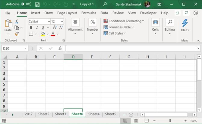
Every Microsoft Excel workbook contains at least one worksheet. You can create multiple worksheets to help organize your data, and each sheet is shown as a tab at the bottom of the Excel window. These tabs make it easier to manage your spreadsheets.
You may have a workbook that contains worksheets for each year for company sales, each department for your retail business, or each month for your bills.
To efficiently manage more than one spreadsheet in a single workbook, we have some tips to help you work with tabs in Excel.
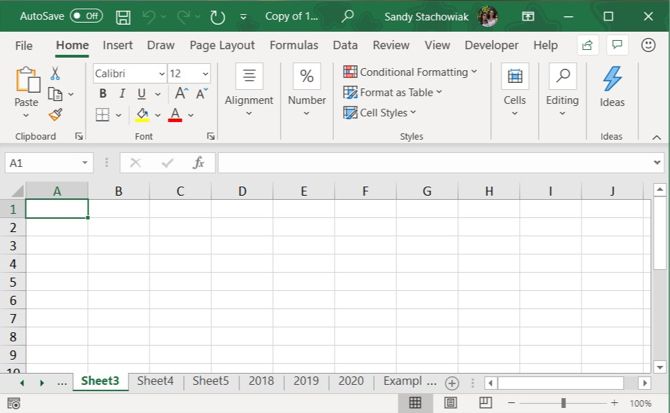
Insert a New Tab
To add another Excel worksheet to your workbook, click the tab after which you want to insert the worksheet. Then, click the plus sign icon on the right of the tab bar.
The new tab is numbered with the next sequential sheet number, even if you’ve inserted the tab in another location. In our example screenshot, our new sheet is inserted after Sheet3, but is numbered Sheet6.
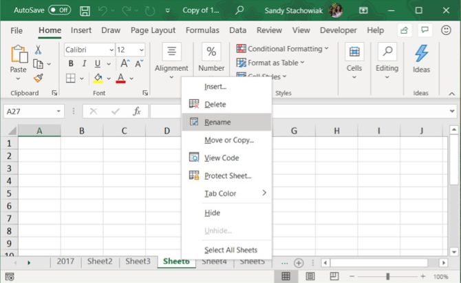
Rename a Tab
New tabs are named Sheet1, Sheet2, etc. in sequential order. If you have multiple worksheets in your workbook, it’s helpful to name each of them to help you organize and find your data.
To rename a tab, either double-click on the tab name or right-click on it and select Rename. Type a new name and press Enter.
Keep in mind that each tab must have a unique name.
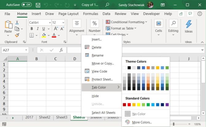
Color a Tab
Along with renaming tabs, you can apply color to them so that they stand out from the rest. Right-click the tab and put your cursor over Tab Color. Select a color from the pop-out window. You’ll notice a nice selection of Theme Colors, Standard Colors, and More Colors if you want to customize the color.
If you have a lot of tabs, they may not all display at once, depending on the size of your Excel window. There are a couple of ways you can scroll through your tabs.
On Windows, you’ll see three horizontal dots on one or both ends of the tab bar. Click the three dots on one end to scroll through the tabs in that direction.
You can also click the right and left arrows on the left side of the tab bar to scroll through the tabs. These arrows also have other uses, as indicated by the popup that displays when you move your cursor over one of them.
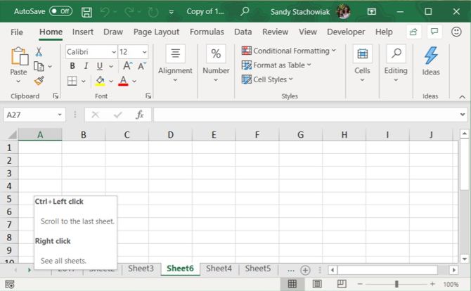
On Mac, you’ll only see the arrows on the left side of the tab bar for scrolling.
View More Tabs on the Tab Bar
On Windows, the scrollbar at the bottom of the Excel window takes up room that could be used for your worksheet tabs. If you have a lot of tabs, and you want to see more of them at once, you can widen the tab bar.
Hover your cursor over the three vertical dots to the left of the scrollbar, until it turns into two vertical lines with arrows. Click and drag the three dots to the right to make the tab bar wider. You’ll start seeing more of your tabs display.
Need to print your Excel sheet? We show you how to format the document to print your spreadsheet on a single page.
Copy or Move a Tab
You can make an exact copy of a tab in the current workbook or in another open workbook, which is useful if you need to start with the same data. You can also move a tab to another location in the same workbook or a different open workbook.
Right-click on the tab and select Move or Copy.
In the Move or Copy dialog box, the currently active workbook is selected by default in the To book dropdown list. If you want to copy or move the tab to a different workbook, make sure that workbook is open and select it from the list. Remember, you can only copy or move tabs to open workbooks.
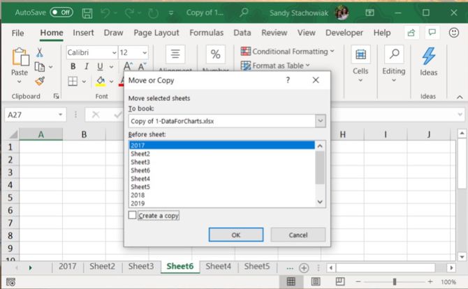
In the Before sheet list box, select the sheet (tab) before which you want to insert the tab. If you’d rather move or copy the tab to the end, pick Move to End.
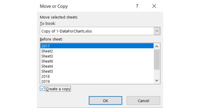
Copying a Tab
If you’re copying the tab, and not moving it, make sure to check the Create a copy box. If you don’t check the Create a copy box, the tab will be moved to the chosen location instead of copied.
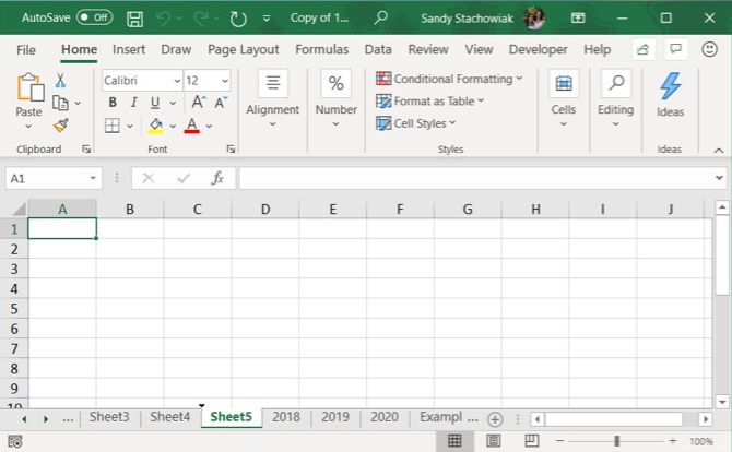
The copied tab will have the same name as the original tab followed by a version number. You can rename the tab as we described in the Rename a Tab section above.
Moving a Tab
If you move the tab, the name will remain the same; a version number is not added.
If you only want to move a tab within the same workbook, you can manually drag it to the new location. Click and hold the tab until you see a triangle on the upper-left corner of the tab. Then, drag the tab until the triangle points to where you want it and then release it.
Delete a Tab
You can delete worksheets (tabs) in your workbook, even those containing data. You will lose the data on a deleted Excel worksheet, and it might cause errors if other worksheets refer to data on the deleted worksheet. So be sure that you actually want to remove the sheet.
Since a workbook must contain at least one spreadsheet, you can’t delete a sheet if it’s the only one in your workbook.
To delete an Excel worksheet, right-click on the tab for the sheet and select Delete.
If the worksheet you’re deleting contains data, a dialog box displays. Click Delete, if you’re sure you want to delete the data on the worksheet.
Hide a Tab
You may want to keep a worksheet and its data in your workbook but not see the sheet. You can take care of this easily by hiding a tab instead of deleting it.
Right-click the tab and choose Hide from the shortcut menu. You’ll see the tab and the sheet disappear from the workbook view.
To make a hidden tab reappear, right-click any tab in the workbook and select Unhide. If you have more than one hidden tab, pick the one you want to see and click OK.
Keep Your Excel Data Organized
Tabs are a great way to keep your Excel data organized and make it easy to find. You can customize the tabs to organize your data in the best way that suits your needs.
You can also speed up navigation and data entry on your worksheets using keyboard shortcuts, as well as use these tips to save time in Excel.