Use LOOKUP, one of the lookup and reference functions, when you need to look in a single row or column and find a value from the same position in a second row or column.
For example, let’s say you know the part number for an auto part, but you don’t know the price. You can use the LOOKUP function to return the price in cell H2 when you enter the auto part number in cell H1.
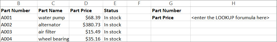
Use the LOOKUP function to search one row or one column. In the above example, we’re searching prices in column D.
Tips: Consider one of the newer lookup functions, depending on which version you are using.
-
Use VLOOKUP to search one row or column, or to search multiple rows and columns (like a table). It’s a much improved version of LOOKUP. Watch this video about how to use VLOOKUP.
-
If you are using Microsoft 365, use XLOOKUP — it’s not only faster, it also lets you search in any direction (up, down, left, right).
There are two ways to use LOOKUP: Vector form and Array form
-
Vector form: Use this form of LOOKUP to search one row or one column for a value. Use the vector form when you want to specify the range that contains the values that you want to match. For example, if you want to search for a value in column A, down to row 6.

-
Array form: We strongly recommend using VLOOKUP or HLOOKUP instead of the array form. Watch this video about using VLOOKUP. The array form is provided for compatibility with other spreadsheet programs, but it’s functionality is limited.
An array is a collection of values in rows and columns (like a table) that you want to search. For example, if you want to search columns A and B, down to row 6. LOOKUP will return the nearest match. To use the array form, your data must be sorted.
Vector form
The vector form of LOOKUP looks in a one-row or one-column range (known as a vector) for a value and returns a value from the same position in a second one-row or one-column range.
Syntax
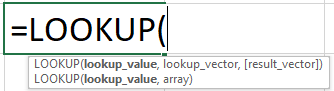
LOOKUP(lookup_value, lookup_vector, [result_vector])
The LOOKUP function vector form syntax has the following arguments:
-
lookup_value Required. A value that LOOKUP searches for in the first vector. Lookup_value can be a number, text, a logical value, or a name or reference that refers to a value.
-
lookup_vector Required. A range that contains only one row or one column. The values in lookup_vector can be text, numbers, or logical values.
Important: The values in lookup_vector must be placed in ascending order: …, -2, -1, 0, 1, 2, …, A-Z, FALSE, TRUE; otherwise, LOOKUP might not return the correct value. Uppercase and lowercase text are equivalent.
-
result_vector Optional. A range that contains only one row or column. The result_vector argument must be the same size as lookup_vector. It has to be the same size.
Remarks
-
If the LOOKUP function can’t find the lookup_value, the function matches the largest value in lookup_vector that is less than or equal to lookup_value.
-
If lookup_value is smaller than the smallest value in lookup_vector, LOOKUP returns the #N/A error value.
Vector examples
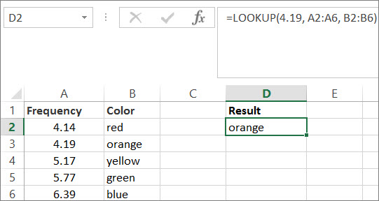
You can try out these examples in your own Excel worksheet to learn how the LOOKUP function works. In the first example, you’re going to end up with a spreadsheet that looks similar to this one:
-
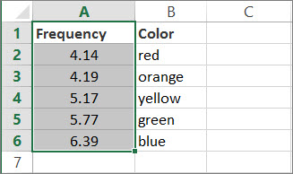
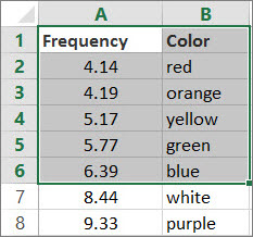
Copy the data in following table, and paste it into a new Excel worksheet.
Copy this data into column A
Copy this data into column B
Frequency
4.14
Color
red
4.19
orange
5.17
yellow
5.77
green
6.39
blue
-
Next, copy the LOOKUP formulas from the following table into column D of your worksheet.
Copy this formula into the D column
Here’s what this formula does
Here’s the result you’ll see
Formula
=LOOKUP(4.19, A2:A6, B2:B6)
Looks up 4.19 in column A, and returns the value from column B that is in the same row.
orange
=LOOKUP(5.75, A2:A6, B2:B6)
Looks up 5.75 in column A, matches the nearest smaller value (5.17), and returns the value from column B that is in the same row.
yellow
=LOOKUP(7.66, A2:A6, B2:B6)
Looks up 7.66 in column A, matches the nearest smaller value (6.39), and returns the value from column B that is in the same row.
blue
=LOOKUP(0, A2:A6, B2:B6)
Looks up 0 in column A, and returns an error because 0 is less than the smallest value (4.14) in column A.
#N/A
-
For these formulas to show results, you may need to select them in your Excel worksheet, press F2, and then press Enter. If you need to, adjust the column widths to see all the data.
Array form
The array form of LOOKUP looks in the first row or column of an array for the specified value and returns a value from the same position in the last row or column of the array. Use this form of LOOKUP when the values that you want to match are in the first row or column of the array.
Syntax
LOOKUP(lookup_value, array)
The LOOKUP function array form syntax has these arguments:
-
lookup_value Required. A value that LOOKUP searches for in an array. The lookup_value argument can be a number, text, a logical value, or a name or reference that refers to a value.
-
If LOOKUP can’t find the value of lookup_value, it uses the largest value in the array that is less than or equal to lookup_value.
-
If the value of lookup_value is smaller than the smallest value in the first row or column (depending on the array dimensions), LOOKUP returns the #N/A error value.
-
-
array Required. A range of cells that contains text, numbers, or logical values that you want to compare with lookup_value.
The array form of LOOKUP is very similar to the HLOOKUP and VLOOKUP functions. The difference is that HLOOKUP searches for the value of lookup_value in the first row, VLOOKUP searches in the first column, and LOOKUP searches according to the dimensions of array.
-
If array covers an area that is wider than it is tall (more columns than rows), LOOKUP searches for the value of lookup_value in the first row.
-
If an array is square or is taller than it is wide (more rows than columns), LOOKUP searches in the first column.
-
With the HLOOKUP and VLOOKUP functions, you can index down or across, but LOOKUP always selects the last value in the row or column.
Important: The values in array must be placed in ascending order: …, -2, -1, 0, 1, 2, …, A-Z, FALSE, TRUE; otherwise, LOOKUP might not return the correct value. Uppercase and lowercase text are equivalent.
-
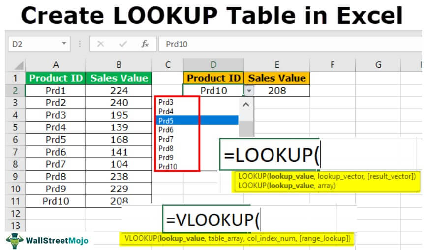
LOOKUP tables in Excel are named tables used with the VLOOKUP function to find any data. When we have a large amount of data and do not know where to look, we can select the table and name it. While using the VLOOKUP function, instead of providing the reference, we can type the table’s name as a reference to look up the value. Such a table is known as a lookup table in Excel.
How to Create a Lookup Table in Excel?
LOOKUP functions are lifesavers in Excel. Based on the available or lookup value, we can fetch the other data in different tables. In Excel, VLOOKUP is the most commonly used LOOKUP function.
This article will discuss some of the important lookup functions in Excel and how to create a lookup table in Excel. Important lookup functions are VLOOKUP and HLOOKUP, V stands for vertical lookup, and H stands for horizontal lookup. We have the function called LOOKUP to look for the data in the table.
You are free to use this image on your website, templates, etc, Please provide us with an attribution linkArticle Link to be Hyperlinked
For eg:
Source: Lookup Table in Excel (wallstreetmojo.com)
We can fetch the available data and other information from different worksheets and workbooks using these LOOKUP functions.
Table of contents
- How to Create a Lookup Table in Excel?
- #1 – Create a Lookup Table Using VLOOKUP Function
- #2 – Use LOOKUP Function to Create a LOOKUP Table in Excel
- #3 – Use INDEX + MATCH Function
- Things to Remember
- Recommended Articles
You can download this Create LOOKUP Table Excel Template here – Create LOOKUP Table Excel Template
#1 – Create a Lookup Table Using VLOOKUP Function
As we said, VLOOKUP is the traditional lookup functionThe VLOOKUP excel function searches for a particular value and returns a corresponding match based on a unique identifier. A unique identifier is uniquely associated with all the records of the database. For instance, employee ID, student roll number, customer contact number, seller email address, etc., are unique identifiers.
read more most users use regularly. Therefore, we will show you how to look for values using this LOOKUP function.
- Lookup Value is nothing but the available value. Based on this value, we are trying to fetch the data from the other table.
- Table Array is simply the main table where all the information resides.
- Col Index Num is nothing but from which column of the table array we want the data. So we need to mention the column number here.
- Range Lookup is nothing but whether you are looking for an exact match or an approximate match. If you are looking for the same match, then FALSE or 0 is the argument. If you are looking for the approximate match, then TRUE or 1 is the argument.
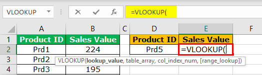
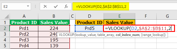
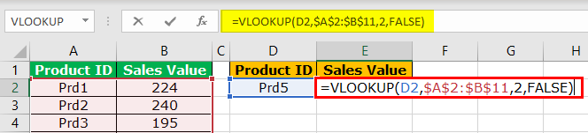
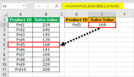
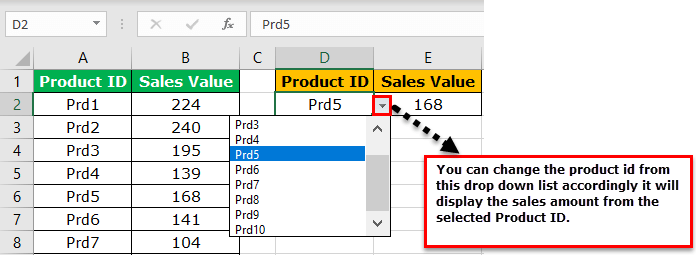
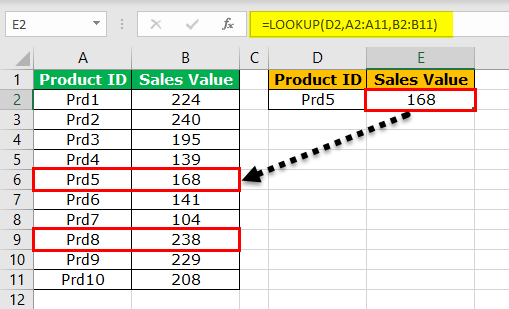
Example of VLOOKUP Function: Assume below is the data you have of product sales and their sales amount.

Now, in cell D2, we have one product ID, and using this product ID, we have to fetch the sales value using VLOOKUP.
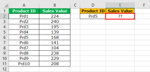
Follow these steps:
- We must apply the VLOOKUP function and open the formula first.

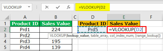
- The first argument is the LOOKUP value. It is our base or available value. So, we must select cell D2 as the reference.

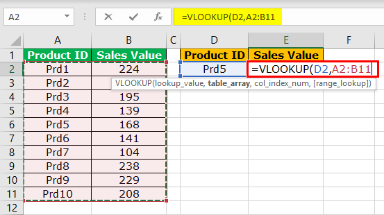
- Next is the table array. It is nothing but our main table where all the data resides. So, select the table array as A2 to B11.

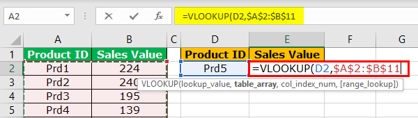
- Now, press the F4 function key to make it an absolute excel reference. It will insert the dollar symbol into the selected cell.

- The next argument is the column index number from the selected table from which column we are looking for the data. In this case, we have chosen two columns, and we need the data from the second column, so we must mention 2 as the argument.

- The final argument is range lookup, i.e., type of lookup. Since we are looking at an exact match, we must select FALSE or insert zero as the argument.

- Close the bracket and press the “Enter” key. We should have the sales value for the product ID Prd5.

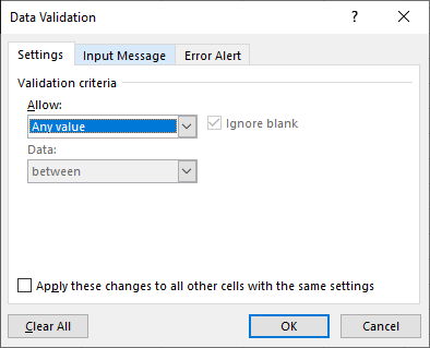
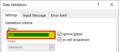
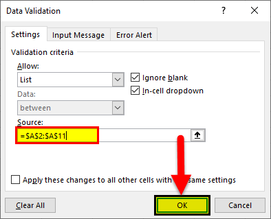
- What if we want the sales data for the product if Prd6. Of course, we can enter directly, but this is not the right approach. Rather, we can create the drop-down list in excel and allow the user to select from the drop-down list. Press ALT + A + V + V in cell D2. It is the shortcut key, which is the shortcut key to create data validation in excel.

- Select the “LIST” from the “Allow:” drop-down.

- In the “SOURCE:” select the Product ID list from A2 to A11.
- Click on the “OK.” We have all the list of products in cell D2 now.

#2 – Use LOOKUP Function to Create a LOOKUP Table in Excel
Instead of VLOOKUP, we can also use the LOOKUP function in excelThe LOOKUP excel function searches a value in a range (single row or single column) and returns a corresponding match from the same position of another range (single row or single column). The corresponding match is a piece of information associated with the value being searched.
read more as an alternative. But, first, let us look at the formula of the LOOKUP function.
- Lookup Value is the base value or available value.
- Lookup Vector is nothing but a lookup value column in the main table.
- Result Vector is nothing but requires a column in the main table.
Let’s apply the formula to understand the logic of the LOOKUP function.
Step 1: We must open the LOOKUP function now.

Step 2: The lookup value is product ID, so select the D2 cell.
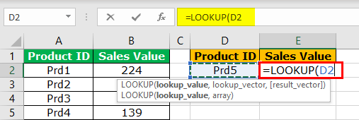
Step 3: The lookup vector is nothing but the product ID column in the main table. So select A1 to A11 as the range.
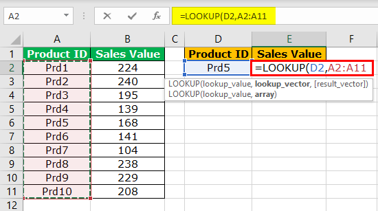
Step 4: Next is the results vector. It is nothing but from which column we need the data to be fetched. In this case, from B1 to B11, we want the data to be brought.
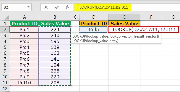
Step 5: Close the bracket and press the “Enter” key to close the formula. We should have sales value for the selected product ID.
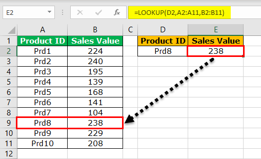
Step 6: Change the product ID to see a different result.
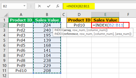
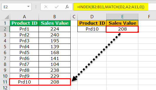
#3 – Use INDEX + MATCH Function
The VLOOKUP function can fetch the data from left to the right, but with the help of the INDEX FunctionThe INDEX function in Excel helps extract the value of a cell, which is within a specified array (range) and, at the intersection of the stated row and column numbers.read more and MATCH formula in excelThe MATCH function looks for a specific value and returns its relative position in a given range of cells. The output is the first position found for the given value. Being a lookup and reference function, it works for both an exact and approximate match. For example, if the range A11:A15 consists of the numbers 2, 9, 8, 14, 32, the formula “MATCH(8,A11:A15,0)” returns 3. This is because the number 8 is at the third position.
read more, we can bring data from anywhere to create a LOOKUP Excel table.
Step 1: Open the INDEX formula ExcelThe INDEX function in Excel helps extract the value of a cell, which is within a specified array (range) and, at the intersection of the stated row and column numbers.read more first.
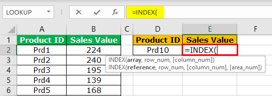
Step 2: Select the result column in the main table for the first argument.
Step 3: To get the row number, we need to apply the MATCH function. Refer to the below image for the MATCH function.
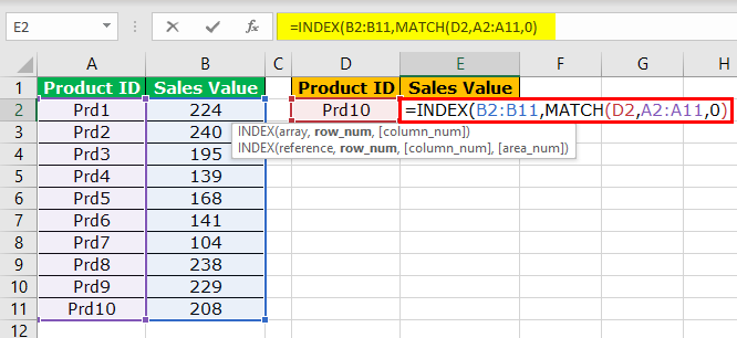
Step 4: Close the bracket and close the formula. We will have results.
Things to Remember
- The LOOKUP should be the same as in the main table in Excel.
- The VLOOKUP function works from left to right, not from right to left.
- In the LOOKUP function, we need to select the result column and need not mention the column index number, unlike VLOOKUP.
Recommended Articles
This article is a guide to the LOOKUP Table in Excel. We discuss creating a LOOKUP table in Excel using VLOOKUP, INDEX, MATCH formulas, practical examples, and a downloadable Excel template. You may also learn more about Excel from the following articles: –
- LOOKUP Formula ExcelThe LOOKUP excel function searches a value in a range (single row or single column) and returns a corresponding match from the same position of another range (single row or single column). The corresponding match is a piece of information associated with the value being searched.
read more - VLOOKUP from Another SheetVlookup is a function that can be used to refer to columns on the same sheet or from another worksheet or workbook. A different workbook or worksheet is used to select the table array and index number.read more
- What are the Alternatives to Vlookup?To reference data in columns from right to left, we can combine the index and match functions, which is one of the best Excel alternatives to Vlookup.read more
- How to Fix VLOOKUP Errors?The top four VLOOKUP errors are — #N/A Error, #NAME? Error, #REF! Error, #VALUE! Error.read more
Lookup Table in Excel (Table of Content)
- Lookup Table in Excel
- How to Use Lookup Table in Excel?
Lookup Table in Excel
The lookup function is not as famous to use as Vlookup and Hlookup; here, we need to understand that it always returns the approximate match when we perform the Lookup function. So there is no true or false argument as it was in Vlookup and Hlookup function. In this topic, we are going to learn about Lookup Table in Excel.
Whenever lookup finds an exact match in the lookup vector, it returns the corresponding value in a given cell, and when it doesn’t find an exact match, it goes back and returns the most recent possible value but from the previous row.
Whenever we have the larger value available in the lookup table or lookup value, it returns the last value from the table, and when we have lower than the lowest, it will return #N/A, as we have understood the same in our previous example.
Remember the below formula for Lookup:
=Lookup(Lookup Value, Lookup Vector, result vector)
Here let us know the arguments:
Lookup Value: The value we are searching
Lookup Vector: Range of lookup value – (1 Row of 1 Column)
Result Vector: Must be the same size as lookup vector; it’s optional
- It can be used in many ways, i.e. Grading of students, Categorizing, retrieve approx. Position, Age group, etc.
- The lookup function assumes Lookup Vector is in ascending order.
How to Use Lookup Table in Excel?
Here we have explained how to use Lookup Table in Excel with the following examples as given below.
You can download this Lookup Table Excel Template here – Lookup Table Excel Template
Example #1
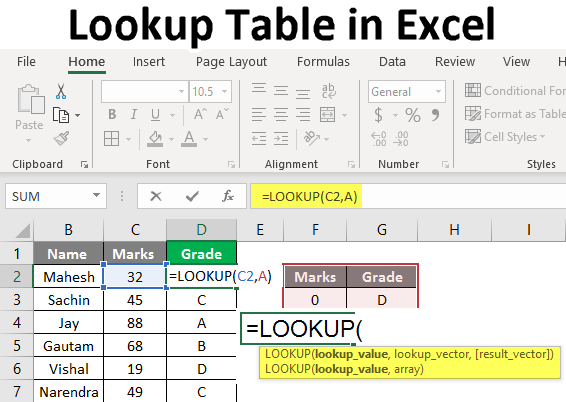
- For this example, we need data from the school students with their names and marks in a particular subject. Now, as we can see in the below image, we have the data of the students as required.
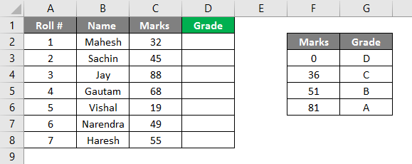
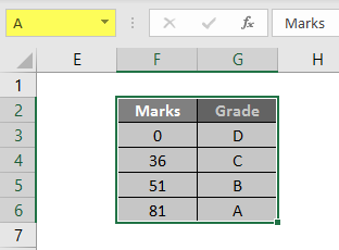
- Here also, we need a lookup vector, the value which defines marks in grades. We can see the image; at the right side of the image, we have decided the criteria for every grade; we will have to make it in ascending order because, as you all know, Look up every time assumes that the data is in ascending order. Now, as you can see, we have entered our formula in D2 Column, =lookup(C2, F2: G6). Here C2 is the lookup value, and F2: G6 is the lookup table/lookup vector.
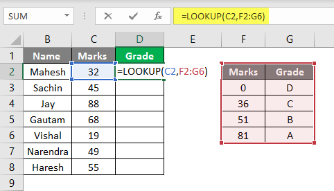
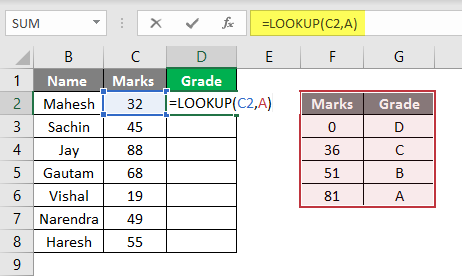
- We can define our lookup table by assigning it a name as any alphabet, let’s assume A, so we can write A instead if it’s range F2: G6. So as per the below image, you can see that we have given the name to our grade table is A.
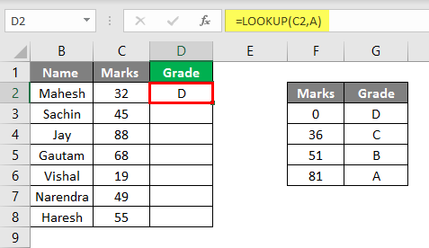
- Now while applying the formula, we can place A instead of its range, the same you can see in the below Image. We have applied the formula as =lookup(C2, A), so here C2 is our lookup value, and A is our lookup table or range of lookup.
- Now we can see that as Mahesh’s marks are 32, so from our lookup/grade table, the lookup will start to look for the value 32 and till 35 marks and its grade as D, so it will show Grade ‘D.’
- If we drag the same till D8, we can see the grades of all the students as per the below image.
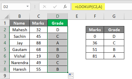
- As per the above image, you can see that we have derived the Grade from the Provided Marks. Similarly, we can use this formula for other purposes; let’s see another example.
Example #2
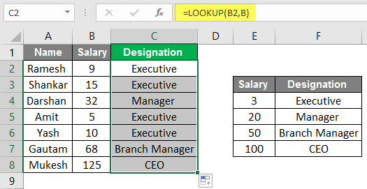
- Like the above table, here we have gathered the data of a company with Name, their salary, and their designations. From the below image, we can see that we have given the name “B” to our lookup table.
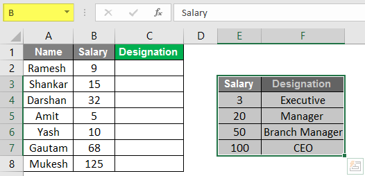
- Now we need the data to be filled in the designation column, So here we will put the formula in C2.
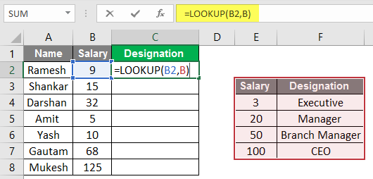
- Here we can see the Result in the Designation Column.
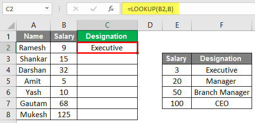
- Now we can see that after dragging we have fetched the designations of the staff according to their salary. We have operated this operation same as a recent example, here instead of marks we have considered the salary of employees and instead of Grade we have considered the designation.
- So we can use this formula for our different purposes academic, personal, and sometimes while making rate cards of a business model to categorize the things in manners of costly things and cheap things.
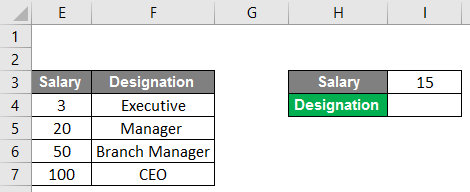
Example #3
- Here as improvisation, we can make a simulator by using a lookup formula; As per the below image, we can see we have used the same data, and instead of the table now, we can put data.
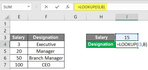
- We can see here in cell no. I4 we have applied the lookup formula, so whenever we put a value in cell no. I3, our lookup formula will look into the data and put the appropriate designation in the cell.
- For example, we have taken the value 15 as salary, so the formula will look up into the table and provide us with the designation according to the table, which is Executive.
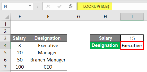
- So accordingly, we can put any value in the cell, But here is a catch, whenever we put a value that is higher than 100, it will show the designation as CEO, and when we put a value lower than 3, it will show #N/A.
Conclusion
The lookup function can lookup value from a single column or a single row of the range. Lookup value always returns a value on a vector; Lookups are of two types of lookup Vector and lookup array. Lookup can be used for various purposes; as we have seen above examples, Lookup can be used in Grading for students we can make age groups and also for the various works.
Things to Remember About Lookup Table in Excel
- While using this function, we have to remember that this function assumes that the lookup table or vector is sorted in ascending order.
- And you must know that this formula is not case sensitive.
- This formula always performs the approximate match, so true or false like arguments will not take place with the formula.
- It can only lookup to a one-column range.
Recommended Articles
This has been a guide to Lookup Table in Excel. Here we have discussed How to Use Lookup Table in Excel along with Examples and a downloadable excel template. You may also look at these useful functions in excel –
- Excel Lookup Function
- LOOKUP Formula in Excel
- VBA LOOKUP
- VLOOKUP Table Array
We can create and use a LOOKUP TABLE in excel for sorting large amount of data. The LOOKUP TABLE allows us to evaluate cells and input an associated comment or remark. The steps below will walk through the process.
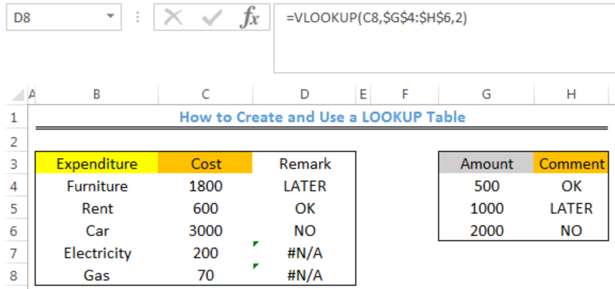 Figure 1- How to Create and Use a LOOKUP Table in Excel
Syntax
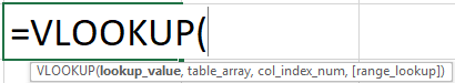
=VLOOKUP(lookup_value,table_array,col_index_num,[range_lookup])
- Lookup_value: This is the value to search for
- Table_array: This is the range to search for the lookup value
- Col_index_num: This number specifies the column where we want the value to be returned from
- Range_lookup: This is used to specify if we want and approximate or exact match of the lookup value. If omitted, VLOOKUP assumes an approximate match
Formula
=VLOOKUP(C4,$G$4:$H$6,2)
Setting up the Data
We will use the LOOKUP TABLE to ascertain based on the comment in Column H if we will proceed with the stated expenditure in COLUMN C as shown in figure 2.
- We will enter the expenditure into Column B
- We will enter the cost into Column C
- Column D contains the Remarks where the results will be returned by VLOOKUP
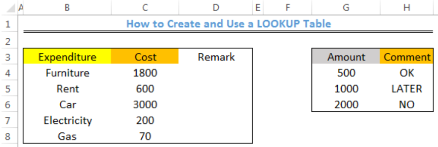 Figure 2 – Setting up the Data
Using the VLOOKUP Function in the LOOKUP TABLE
- We will click on Cell D4
- We will insert the formula below into Cell D4
=VLOOKUP(C4,$G$4:$H$6,2) - We will press the enter key
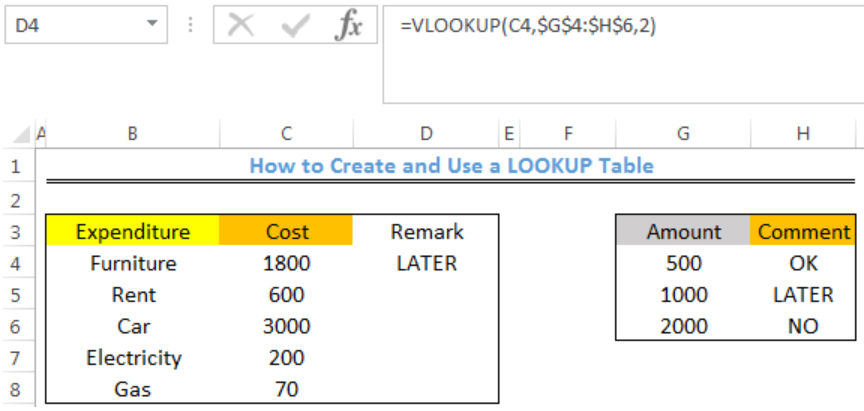 Figure 3- VLOOKUP result for Remarks about the Furniture Expenditure
- We will click on Cell D4 again
- We will double click on the fill handle tool which is the small plus sign you see at the bottom right of Cell D4. Select and drag down to copy the formula to Cell D8
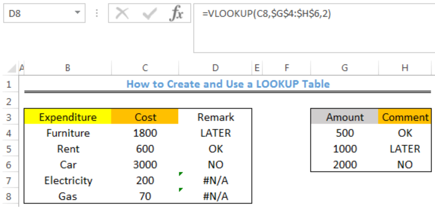 Figure 4- VLOOKUP results for Remarks about all Expenditure
Note
- The VLOOKUP function assumes that the lookup table is sorted in ascending order
- If the lookup_value is greater than every value in the lookup table, the LOOKUP function matches the last value
- If the lookup_value is less than all values in the lookup table, the VLOOKUP function returns the #N/A error
Instant Connection to an Expert through our Excelchat Service
Most of the time, the problem you will need to solve will be more complex than a simple application of a formula or function. If you want to save hours of research and frustration, try our live Excelchat service! Our Excel Experts are available 24/7 to answer any Excel question you may have. We guarantee a connection within 30 seconds and a customized solution within 20 minutes.
Data lookup is quite simply the process where values in Excel are scanned until certain results are found. In Excel 2016, there are two main formulas for looking up the data you have in a worksheet. There is VLookup where the V stands for vertical, and there is HLookup where the H stands for Horizontal.
The Basic VLookup Formula
Below is the basic VLookup formula.

Inside the brackets, you will see the information that Excel asks us to enter into the formula.
You can also go to the Formulas tab, click the Lookup & Reference button, then select VLookup.
You will then see this dialogue box:
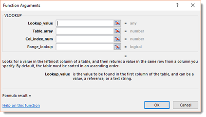
The benefit of using the dialogue box when entering a formula is the bit of instruction that Excel gives you for each field. If you are newer to Excel, it is recommended that you use the Function Arguments dialogue box to create your formulas. It is a lot less trial and error that way.
For the time being, however, let’s look the formula in our worksheet again.
-
Lookup_value is the value that we want to look up.
-
The table_array is the table where the data will be retrieved. This value can be a range or the name of a range.
-
Col-index_num is the column number in the table. The first column in your table is column 1.
-
Range_Lookup is typically true for false. True will give you a near match. If you want to find an exact match, it is false.
Let’s learn how to use the VLookup formula.
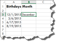
Take a look at our worksheet below.
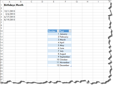
On the left, we have birthdays listed. We know that 12 means December, and we could use the MONTH function to fill in December for us, but instead we want the text value.
On the right, we have created a lookup table. We are going to use a VLookup to find the text value.
We start by entering the VLOOKUP function, then open brackets.
The first piece of information we must supply is the lookup value. We know the lookup value is the month located in Column A (the first column), but we must use the MONTH function to specify this, as shown below.
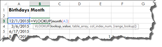
Next, we add a comma, then for the table_array, we are going to highlight the cells in the table; however, we do not highlight the column headers.
Enter another comma.
Now, for the col_index_num. Ours is Column 2. We then enter another comma.
Since we want the exact match, we enter FALSE.
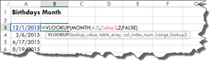
Close the brackets, then push Enter.
About Lookup Tables
A lookup table is created by simply creating a table in Excel. It is used as a master list of sorts, and you will use it to locate data that you need to find using search criteria that you will enter into your lookup formula. You can use a huge table of data that you have created as your lookup table. You do not have to create a lookup table just to use either the VLookup or HLookup functions.
For example, let’s say you have a table within a spreadsheet that contains 15,000 customer names, complete with address, billing information, shipping information, anniversary dates, and etc. You can use a lookup formula to find specific data within the table. If you wanted to find the address, for example, you could create a lookup formula to find that within your table of data.
Naming Lookup Table Data
If you are looking up data that may be on different worksheets within a workbook, it makes it easier if you name the data you are going to be searching.
This is easy to do.
Go to the lookup table data. Click anywhere in the data, then press CTRL+A. This selects all of the data.
Next, go to the Formula tab.
Click the Define Name button in the Defined Names group.
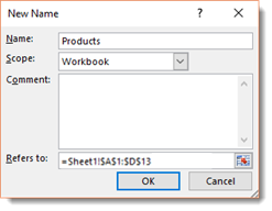
Enter a name for the group. The scope is workbook.
Click OK.
Now, when you enter the table_array information into your data lookup, you can simply enter this name. In our case, it is products. You will see it appear in a dropdown menu.
Please note that if you add data to the end of a lookup table after you have named it, then enter the name of the data into Excel (we named ours Products), the formula will not retrieve that data because it is not part of your named data.
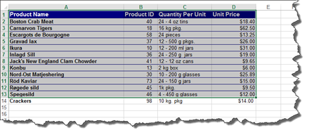
We entered another product to our product list below.
Now we can go to our Name box, and choose the name of your data.

As you can see, the last row is not included.
If you add rows or columns to a lookup table after you have named it, insert the data into the existing data table. Do not put it at the very beginning or the very end. Otherwise, you will have to rename it, then change your lookup formula.
Look what happens when we insert the new row above our last row.
It is now included with the data.
However, you can always add extra blank rows in your lookup table so that you have room to add new things at the end.
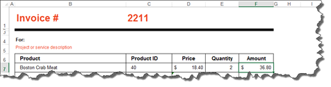
VLOOKUP: A Real Example
It is important that you understand exactly how VLOOKUP works. For that reason, we are going to show a more realistic example.
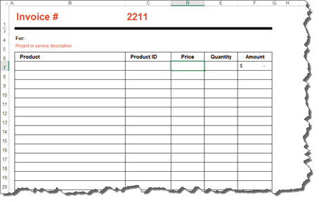
Below we have an Excel invoice. This is just one of the pre-built templates that we are going to use.
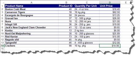
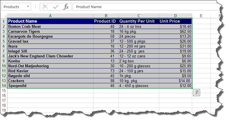
We also have a product list in another worksheet.
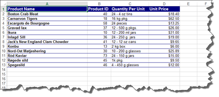
We are going to use VLOOKUP to find the product ID and the price per unit for our invoice.
Take a look at our invoice again.
We have entered in Crab Meat as the first product sold.
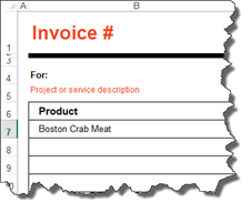
Now, we are going to use VLOOKUP to find the product ID.
Enter your VLookup formula in the cell for the product ID.
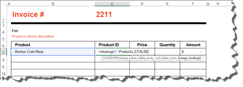
Notice that we entered in Products for the table_array.
Hit Enter.
You should now have the product ID in the cell.
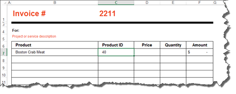
Now let’s do the price.
As we fill in our formula, notice that when we get to table_array and type in the name for our data, it appears in a dropdown list.
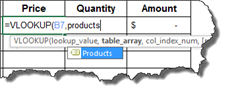
Finish entering in the formula.
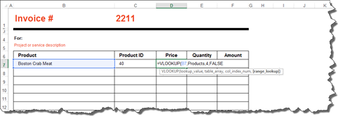
Close the brackets when you are finished entering the formula, then press Enter.
About HLOOKUP
Whereas VLOOKUP is vertical lookup, HLOOKUP is horizontal lookup. However, vertical or horizontal lookups do not refer to the table in which you want to place the results. Instead, it refers to the table in which you are using to search for data.
When you use the HLOOKUP function, you are looking for data horizontally. In VLOOKUP, we looked in a column for data. Columns are vertical. In HLOOKUP, you search rows. Instead of entering the column number, you will enter the row number, as shown below.
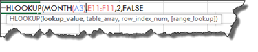
Add the end bracket to the formula, then press Enter.
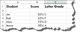
Working with Near Matches
Let’s talk about range lookup in the VLOOKUP and HLOOKUP formulas. As we already have learned, if you enter FALSE as the range lookup, Excel will return the exact match for the results.
However, if you use the TRUE argument for a lookup, it will use the nearest match that is of the next largest value if an exact match is not found.
For our lookup table, we have a grading scale.
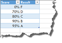
We are going to use VLOOKUP to input the letter grade.
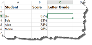
Below is our formula. Notice that we named our data «score.»
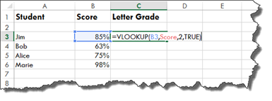
Hit Enter.
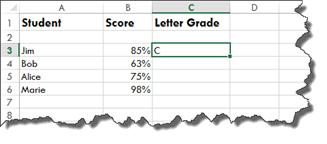
Now, drag the handle in the lower right hand corner of the results cell to fill in the rest of the data.
When There is Missing Data in a Lookup
If you use VLOOKUP or HLOOKUP, and Excel cannot find the data you are looking for, you will see this message appear in the cell after you press Enter to see results.

What you will want to do if you see this message is to run an IF statement to make sure the data really is not there.
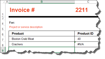
Let’s use our invoice and product list as an example. We are going to create the formula, product the #N/A message, then run the IF statement.
In our invoice below, we have entered a product that we know does not exist in our product list.
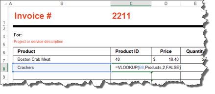
We are going to hit Enter to see the results of the formula.
As we already knew would happen, Excel can’t find the results.
To make sure the lookup is correct, we are going to modify our formula so we can run an IF statement.
To start with, we typed IF after the = for the IF statement, then we entered an opening bracket and typed «isna.»

We also added a closing bracket to the end to close the IF statement and our VLOOKUP. As you can see above, our VLOOKUP formula sits inside the «isna» formula.
If the result really is NA, we want Excel to give us 0 as a result because there is not a product number.
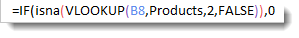
If there is a value, we want it to do a VLOOKUP again, so we copy and paste the VLOOKUP in after placing another comma.

As you can see, we then get a zero because the data is indeed missing.
Nesting a Lookup Within a Lookup
You can nest a lookup within a lookup to go through multiple tables and pull out a value.
For example, in our worksheet shown below, we have a list of employees with the years that they have worked for our fictional company.
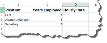
We want to use our lookup tables to determine their hourly rate of pay.
That said, our fictional company determines an employee’s hourly pay by their job classification, then the number of years they have been on the job.
We have two data tables for that.
Here is the first. We named it «class.»
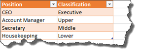
As you can see, this table lists the various job positions in the company, then lists the classification for each position.
Here is our second table. We named it «salary.»
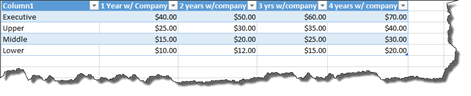
This table lists the different classifications, then the hourly rate of pay for those classifications based on the number of years the employee has been on the job.
To figure out the hourly rate for our worksheet, we will use nested VLOOKUPS.
Let’s start out by using VLOOKUP to find the job classification for the first employee in our list.
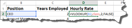
Now we will nest this VLOOKUP inside another VLOOKUP.
To do this, we will put the cursor after the equal sign in our formula, then type VLOOKUP again, followed by an opening bracket.
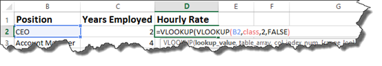
Put a comma after the closing bracket, then enter your table array for the new VLOOKUP, the column number, then FALSE for an exact match – as shown below.
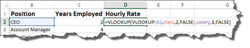
Hit Enter.
Our formula should now show the hourly rate for the employee.
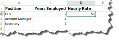
If we consult with the tables, we see that $50.00 is indeed the hourly rate for a CEO who has been with the company for two years.
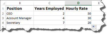
Now we can figure out the hourly rate for the rest of the employees.
The IF Function
The IF function helps to determine what will be displayed to those who view your worksheets in Excel. Because of its purpose, it is one of the most important functions you will learn. IF functions can be used to add comments to your data. They can also be used to hide errors in calculations.
About the IF Function
The syntax for the IF function is =IF. This lets Excel know that it is an IF function.
Then, we begin the formula that Excel will use to produce the results we want.
We start with an opening bracket:

Next, we add the evaluation criteria. For example, is six greater than three? The evaluation criteria asks a question. The question has two outcomes. If the answer (or outcome) is correct, such as «Yes, six is greater than three,» then the answer is true. If not, it is false.
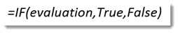
If it is true, we put what happens when the answer is true.
If it is false, we put what happens when it is false.
In the worksheet below, we have a list of employees, followed by the rating they received as part of their annual review.
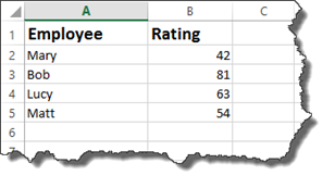
Now, we want to add another column called Comments. In this column, we want to add comments about the scores. This way, when a manager looks at the worksheet, he/she does not need to worry themselves with the actual rating – and what that means. They can simply look in comments.
To add a comment based on the rating, we are going to use the IF function.
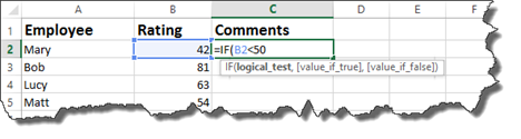
We have started the formula in the snapshot above.
We have said if the employee’s rating is less than fifty…
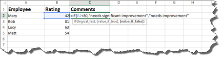
Now we enter what happens.
If it is correct that the employee’s rating is less than fifty, the comment should be «needs significant improvement. However, if it is false and if the rating is not less than fifty, the comment should be needs improvement.
Notice that we use quotation marks to enter the comments into the formula.
Now, add an end bracket, then push Enter.
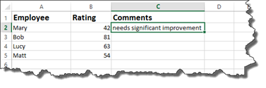
Since this contains a formula where all are cell references are relative, you can use the handle in the lower right corner of the cell, then drag it down to complete the comments for the other employees.
You can also use the IF function to hide Excel error messages.
Let’s show you what we mean by taking a look at the worksheet below.
In this worksheet, we have a formula that will divide cell C2 by cell D2.
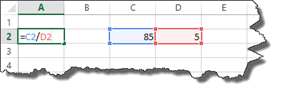
If we push enter in cell A2, it will give us the answer.
However, let’s say the data in cell D2 is missing.
When we push Enter, we see an error message.
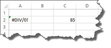
We can use the IF function to hide this error message.
To do this, we write the formula below:
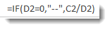
Let’s translate what it says. If D2 equals 0, enter two dashes into cell A2 where we have our formula. If it does not equal zero, then go ahead and divide cell C2 by D2.
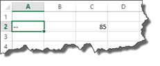
If we would put the number five back into cell D2 and leave the IF formula in place, we would see the answer to C2/D2.
Here is our worksheet below. We have hidden the error message with two dashes.
NOTE: All of the IF functions appear under the Formulas tab and by clicking the Logical button. From there, you can access the Function Arguments dialogue box.
The IFNA and IFERROR Functions
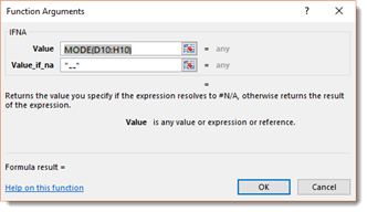
The IFNA function tells Excel what to do if an #NA error is produced, whereas the isna tells Excel what to do if the returned value is #NA.
The #NA error appears in a cell when a value is not available to a formula.
If in our worksheet below, we wanted to find the mode, we would enter this formula:

When we push Enter, the result is displayed.

However, if we went back and changed the second instance of the number four to a six, we would see an #NA error because the value needed is not available to determine the mode.

To avoid #NA values from appearing, we could use the new IFNA function.
It would be entered like this:

All of the IF functions appear under the Formulas tab and by clicking the Logical button. The easiest way to use the IFNA function is to click the Logical button, then select IFNA.
Below you can see the dialogue box for the IFNA function.
The IFERROR function can be used as a general «cover all» for any errors that might appear in your data. You can use it to specify what will be entered if any error occurs in the calculation of a formula.
It is written the same way as an IF function. However, instead of writing IF, you would write IFERROR. You can access the dialogue box for IFERROR by going to the Logical button under the Formulas tab.
Nesting IF Statements
Just as with VLOOKUPs and HLOOKUPs, you can nest an IF statement within an IF statement.
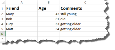
In our worksheet below, we have a list of friends, along with their ages.
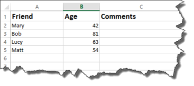
We could create a simple IF formula to enter comments.
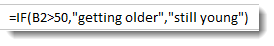
This says if the age is greater than 50, then the comment is getting older. If it is less than 50, then they are still young.
If we nest an IF statement within the current IF statement, we would keep the evaluation criteria, but we would replace one of the outcomes with our new IF statement. However, keep in mind, then when you nest an IF statement, you do not need another equal sign.
Take a look at our new formula below:
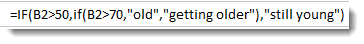
We have our original IF statement intact. We have highlighted the first part of it below.
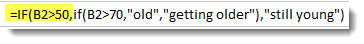
If the age is greater than 50, followed by the two outcomes.
As you can see in our formula above, the TRUE outcome has another IF statement.
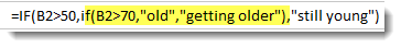
The nested IF statement tells Excel that if the age is greater than 70, enter the comment «old.» If it is not, enter getting older.
Our worksheet is shown below with the nested IF statements determining what comment is displayed.
Now, let’s break this down into easy to understand terms.
When you enter the formula above with a nested IF statement, Excel reads the first IF statement. It looks at your criteria, then the outcomes for the criteria.
If the outcome for the first IF statement is true, Excel is then going to perform another IF statement to determine what appears in the comments. It will put «old» if the age is greater than 70. It will put getting older if it is not greater than 70. It is very important to remember that these two outcomes both serve as your TRUE outcome for the first IF function.
Now, if your original IF statement returns a FALSE outcome, then Excel will enter «still young.»
A nested IF statement gives you a way to enter more than one response for an outcome.
We used a nested if statement for the TRUE outcome. However, you can also use a nested IF statement for a FALSE outcome.
If the nested IF statements are still confusing to you, remember it this way: the nested IF statement provides two additional outcomes for either the TRUE or FALSE outcome of your original IF statement.
Using the AND Operator in an IF Statement
You use the AND operator within an IF statement if you have more than one criteria that needs to be true. Using the AND operator can sometimes be easier to write than multiple nested IF statements.
Take a look at the worksheet below.
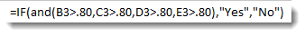
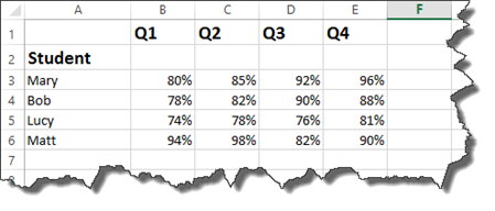
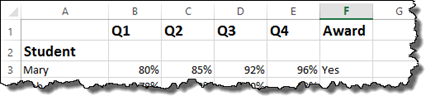
In it, we have a list of students and their grades for the four grading periods.

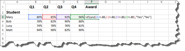
Each student must have earned greater than 80% in each quarter in order to receive an award. We will use the AND operator to set this as criteria.
Take a look at how at the formula bar to see how we wrote this.
Now, let’s examine it.
We start out by starting the IF statement with =IF, then the open bracket.
Next, we write AND for the AND operator. The criteria then is placed within brackets. Notice that we have four sets of criteria. The criteria is that each quarter’s grades must be greater than 80%. Also notice that all percentages have been converted to decimals when entered in as criteria.
After you have entered the criteria in brackets, you can enter your TRUE and FALSE values. We want the cell to display «Yes» if the criteria is met. We want it do display «No» if it is not met. We then type in an end bracket to close the IF statement.
Press Enter.
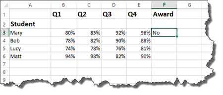
As you can see above, student Mary had one grade that was 80%. All of the grades had to be above 80% to meet our criteria, so a NO was returned.
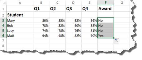
You can now drag the handle in the cell down to complete the worksheet for all students.
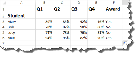
Using the OR Operator in an IF Statement
The OR operator works in the same way as the AND, except it says if one of the criteria listed is true, then the outcome for TRUE is what is displayed.
Let’s look at our worksheet.
This time, we want to say if the grade for Q1, Q2, Q3, or Q4 is greater than 90%, then the student gets the award.
You enter it in the same way you did with the IF statement and the AND operator, expect you type OR instead of AND.
Press Enter.
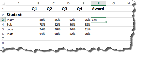
You can then complete the worksheet.
Now let’s make it a bit more complicated.
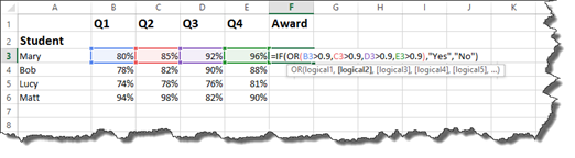
Now we want to say that in order to get the award, the average of all four quarters must be greater than 90% OR at least one of the quarters must be greater than 95%.
In other words, the average of the quarters must be greater than 90%. Or Q1, Q2, Q3, or Q4 must be higher than 95%.
This is the perfect time for you to test our your ability writing formulas by entering the formula into the cell.
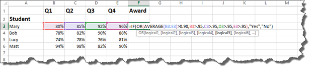
Press Enter.
Using the NOT Operator
The NOT operator is used in conjunction with the AND or OR operator.
The best way to explain how the NOT operator works is to show you the NOT operator in action.
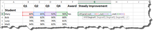
Working with our students and grades again, we want to determine if the grades have improved each quarter.
To do that, we are going to use the IF statement with the AND operator since we are using multiple criteria.
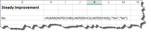
We will use the NOT operator to make sure Q1 is not higher than Q2. Q2 must be greater than Q1.
In addition, Q3 must be greater than Q2, and Q4 must be greater than Q3.
We have started the write it below:
Let’s finish.
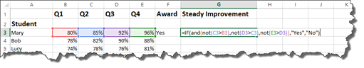
Hit Enter.
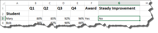
We can see there is not steady improvement.
Remember: The NOT Operator is used within AND or IF options. You must use the NOT operator for each piece of criteria. You cannot type in the NOT operator once, then use it for all criteria.
Displaying Cell Formulas In Another Cell
Starting with Excel 2016, you can display the formula from one cell in another. In our worksheets so far, we could view the formula in a cell by double clicking on the cell. However, once we pressed Enter or tabbed out of a cell, we could not see the formula unless we looked in the Formula Bar.
To display a formula from one cell in another cell, go to the cell where you want to formula to appear.
You will use the FORMULATEXT function.
Type the equal sign, followed by formula text.
Enter an open bracket, then click the cell that contains the formula you want to display.
Add the closing bracket.
For our example, we are going to display the formula in cell G3 in sell H3.
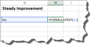
Press Enter.