What are excel data tables created from - Word и Excel - помощь в работе с программами

Содержание

Data Tables
One Variable Data Table
Two Variable Data Table
Calculate multiple results by using a data table
Need more help?

Data Tables

Instead of creating different scenarios, you can create a data table to quickly try out different values for formulas. You can create a one variable data table or a two variable data table.

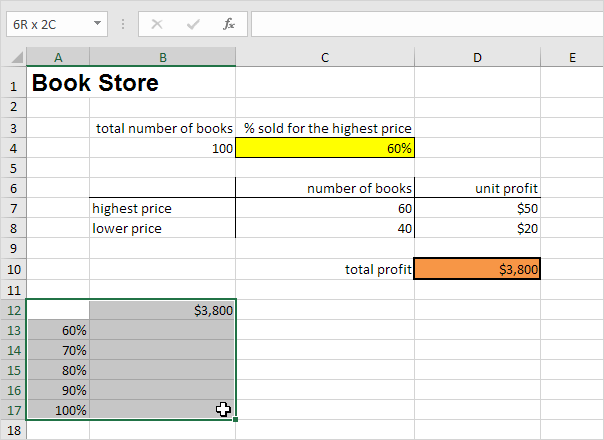
Assume you own a book store and have 100 books in storage. You sell a certain % for the highest price of $50 and a certain % for the lower price of $20. If you sell 60% for the highest price, cell D10 below calculates a total profit of 60 * $50 + 40 * $20 = $3800.

One Variable Data Table

To create a one variable data table, execute the following steps.

1. Select cell B12 and type =D10 (refer to the total profit cell).

2. Type the different percentages in column A.

3. Select the range A12:B17.

We are going to calculate the total profit if you sell 60% for the highest price, 70% for the highest price, etc.

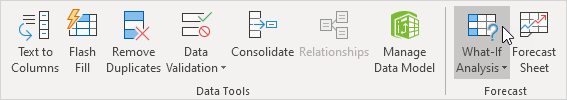
4. On the Data tab, in the Forecast group, click What-If Analysis.

5. Click Data Table.

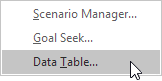
6. Click in the ‘Column input cell’ box (the percentages are in a column) and select cell C4.

We select cell C4 because the percentages refer to cell C4 (% sold for the highest price). Together with the formula in cell B12, Excel now knows that it should replace cell C4 with 60% to calculate the total profit, replace cell C4 with 70% to calculate the total profit, etc.

Note: this is a one variable data table so we leave the Row input cell blank.

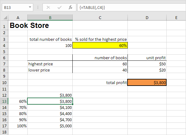
Conclusion: if you sell 60% for the highest price, you obtain a total profit of $3800, if you sell 70% for the highest price, you obtain a total profit of $4100, etc.

Note: the formula bar indicates that the cells contain an array formula. Therefore, you cannot delete a single result. To delete the results, select the range B13:B17 and press Delete.

Two Variable Data Table

To create a two variable data table, execute the following steps.

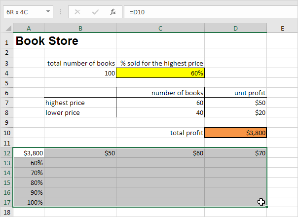
1. Select cell A12 and type =D10 (refer to the total profit cell).

2. Type the different unit profits (highest price) in row 12.

3. Type the different percentages in column A.

4. Select the range A12:D17.

We are going to calculate the total profit for the different combinations of ‘unit profit (highest price)’ and ‘% sold for the highest price’.

5. On the Data tab, in the Forecast group, click What-If Analysis.

6. Click Data Table.

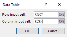
7. Click in the ‘Row input cell’ box (the unit profits are in a row) and select cell D7.

8. Click in the ‘Column input cell’ box (the percentages are in a column) and select cell C4.

We select cell D7 because the unit profits refer to cell D7. We select cell C4 because the percentages refer to cell C4. Together with the formula in cell A12, Excel now knows that it should replace cell D7 with $50 and cell C4 with 60% to calculate the total profit, replace cell D7 with $50 and cell C4 with 70% to calculate the total profit, etc.

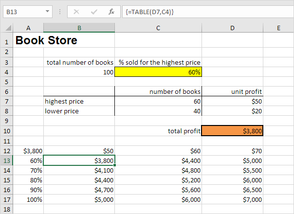
Conclusion: if you sell 60% for the highest price, at a unit profit of $50, you obtain a total profit of $3800, if you sell 80% for the highest price, at a unit profit of $60, you obtain a total profit of $5200, etc.

Note: the formula bar indicates that the cells contain an array formula. Therefore, you cannot delete a single result. To delete the results, select the range B13:D17 and press Delete.

Источник

Calculate multiple results by using a data table

A data table is a range of cells in which you can change values in some of the cells and come up with different answers to a problem. A good example of a data table employs the PMT function with different loan amounts and interest rates to calculate the affordable amount on a home mortgage loan. Experimenting with different values to observe the corresponding variation in results is a common task in data analysis.

In Microsoft Excel, data tables are part of a suite of commands known as What-If analysis tools. When you construct and analyze data tables, you are doing what-if analysis.

What-if analysis is the process of changing the values in cells to see how those changes will affect the outcome of formulas on the worksheet. For example, you can use a data table to vary the interest rate and term length for a loan—to evaluate potential monthly payment amounts.

Note: You can perform faster calculations with data tables and Visual Basic for Applications (VBA). For more information, see Excel What-If Data Tables: Faster calculation with VBA.

Types of what-if analysis

There are three types of what-if analysis tools in Excel: scenarios, data tables, and goal-seek. Scenarios and data tables use sets of input values to calculates possible results. Goal-seek is distinctly different, it uses a single result and calculates possible input values that would produce that result.

Like scenarios, data tables help you explore a set of possible outcomes. Unlike scenarios, data tables show you all the outcomes in one table on one worksheet. Using data tables makes it easy to examine a range of possibilities at a glance. Because you focus on only one or two variables, results are easy to read and share in tabular form.

A data table cannot accommodate more than two variables. If you want to analyze more than two variables, you should instead use scenarios. Although it is limited to only one or two variables (one for the row input cell and one for the column input cell), a data table can include as many different variable values as you want. A scenario can have a maximum of 32 different values, but you can create as many scenarios as you want.

Create either one-variable or two-variable data tables, depending on the number of variables and formulas that you need to test.

One-variable data tables

Use a one-variable data table if you want to see how different values of one variable in one or more formulas will change the results of those formulas. For example, you can use a one-variable data table to see how different interest rates affect a monthly mortgage payment by using the PMT function. You enter the variable values in one column or row, and the outcomes are displayed in an adjacent column or row.

In the following illustration, cell D2 contains the payment formula, =PMT(B3/12,B4,-B5), which refers to the input cell B3.

Two-variable data tables

Use a two-variable data table to see how different values of two variables in one formula will change the results of that formula. For example, you can use a two-variable data table to see how different combinations of interest rates and loan terms will affect a monthly mortgage payment.

In the following illustration, cell C2 contains the payment formula, =PMT(B3/12,B4,-B5), which uses two input cells, B3 and B4.

Data table calculations

Whenever a worksheet recalculates, any data tables will also recalculate—even if there has been no change to the data. To speed up calculation of a worksheet that contains a data table, you can change the Calculation options to automatically recalculate the worksheet but not the data tables. To learn more, see the section Speed up calculation in a worksheet that contains data tables.

A one-variable data table contain its input values either in a single column (column-oriented), or across a row (row-oriented). Any formula in a one-variable data table must refer to only one input cell.

Follow these steps:

Type the list of values that you want to substitute in the input cell—either down one column or across one row. Leave a few empty rows and columns on either side of the values.

Do one of the following:

If the data table is column-oriented (your variable values are in a column), type the formula in the cell one row above and one cell to the right of the column of values. This one-variable data table is column-oriented, and the formula is contained in cell D2.

If you want to examine the effects of various values on other formulas, enter the additional formulas in cells to the right of the first formula.

If the data table is row-oriented (your variable values are in a row), type the formula in the cell one column to the left of the first value and one cell below the row of values.

If you want to examine the effects of various values on other formulas, enter the additional formulas in cells below the first formula.

Select the range of cells that contains the formulas and values that you want to substitute. In the figure above, this range is C2:D5.

On the Data tab, click What-If Analysis > Data Table (in the Data Tools group or Forecast group of Excel 2016).

Do one of the following:

If the data table is column-oriented, enter the cell reference for the input cell in the Column input cell field. In the figure above, the input cell is B3.

If the data table is row-oriented, enter the cell reference for the input cell in the Row input cell field.

Note: After you create your data table, you might want to change the format of the result cells. In the figure, the result cells are formatted as currency.

Formulas that are used in a one-variable data table must refer to the same input cell.

Follow these steps

Do either of these:

If the data table is column-oriented, enter the new formula in a blank cell to the right of an existing formula in the top row of the data table.

If the data table is row-oriented, enter the new formula in a empty cell below an existing formula in the first column of the data table.

Select the range of cells that contains the data table and the new formula.

On the Data tab, click What-If Analysis > Data Table (in the Data Tools group or Forecast group of Excel 2016).

Do either of the following:

If the data table is column-oriented, enter the cell reference for the input cell in the Column input cell box.

If the data table is row-oriented, enter the cell reference for the input cell in the Row input cell box.

A two-variable data table uses a formula that contains two lists of input values. The formula must refer to two different input cells.

Follow these steps:

In a cell on the worksheet, enter the formula that refers to the two input cells.

In the following example—in which the formula starting values are entered in cells B3, B4, and B5, you type the formula =PMT(B3/12,B4,-B5) in cell C2.

Type one list of input values in the same column, below the formula.

In this case, type the different interest rates in cells C3, C4, and C5.

Enter the second list in the same row as the formula—to its right.

Type the loan terms (in months) in cells D2 and E2.

Select the range of cells that contains the formula (C2), both the row and column of values (C3:C5 and D2:E2), and the cells in which you want the calculated values (D3:E5).

In this case, select the range C2:E5.

On the Data tab, in the Data Tools group or Forecast group (in Excel 2016), click What-If Analysis > Data Table (in the Data Tools group or Forecast group of Excel 2016).

In the Row input cell field, enter the reference to the input cell for the input values in the row.
Type cell B4 in the Row input cell box.

In the Column input cell field, enter the reference to the input cell for the input values in the column.
Type B3 in the Column input cell box.

Example of a two-variable data table

A two-variable data table can show how different combinations of interest rates and loan terms will affect a monthly mortgage payment. In the figure here, cell C2 contains the payment formula, =PMT(B3/12,B4,-B5), which uses two input cells, B3 and B4.

When you set this calculation option, no data-table calculations occur when a recalculation is done on the entire workbook. To manually recalculate your data table, select its formulas and then press F9.

Follow these steps to improve calculation performance:

Click File > Options > Formulas.

In the Calculation options section, under Calculate, click Automatic except for data tables.

Tip: Optionally, on the Formulas tab, click the arrow on Calculation Options, then click Automatic Except Data Tables (in the Calculation group).

You can use a few other Excel tools to perform what-if analysis if you have specific goals or larger sets of variable data.

If you know the result to expect from a formula, but don’t know precisely what input value the formula needs to get that result, use the Goal-Seek feature. See the article Use Goal Seek to find the result you want by adjusting an input value.

You can use the Excel Solver add-in to find the optimal value for a set of input variables. Solver works with a group of cells (called decision variables, or simply variable cells) that are used in computing the formulas in the objective and constraint cells. Solver adjusts the values in the decision variable cells to satisfy the limits on constraint cells and produce the result you want for the objective cell. Learn more in this article: Define and solve a problem by using Solver.

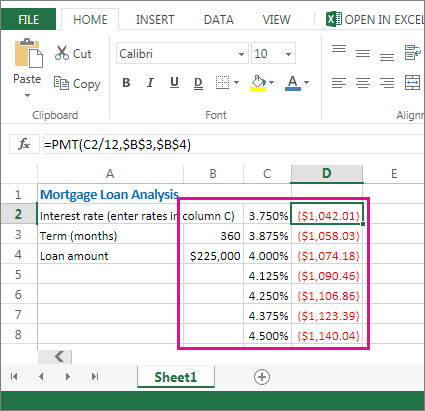
By plugging different numbers into a cell, you can quickly come up with different answers to a problem. A great example is using the PMT function with different interest rates and loan periods (in months) to figure out how much of a loan you can afford for a home or a car. You enter your numbers into a range of cells called a data table.

Here, the data table is the range of cells B2:D8. You can change the value in B4, the loan amount, and the monthly payments in column D automatically update. Using a 3.75% interest rate, D2 returns a monthly payment of $1,042.01 using this formula: =PMT(C2/12,$B$3,$B$4).

You can use one or two variables, depending on the number of variables and formulas you want to test.

Use a one-variable test to see how different values of one variable in a formula will change the results. For example, you can change the interest rate for a monthly mortgage payment by using the PMT function. You enter the variable values (the interest rates) in one column or row, and the outcomes are displayed in a nearby column or row.

In this live workbook, cell D2 contains the payment formula =PMT(C2/12,$B$3,$B$4). Cell B3 is the variable cell, where you can plug in a different term length (number of monthly payment periods). In cell D2, the PMT function plugs in the interest rate 3.75%/12, 360 months, and a $225,000 loan, and calculates a $1,042.01 monthly payment.

Use a two-variable test to see how different values of two variables in a formula will change the results. For example, you can test different combinations of interest rates and number of monthly payment periods to calculate a mortgage payment.

In this live workbook, cell C3 contains the payment formula, =PMT($B$3/12,$B$2,B4), which uses two variable cells, B2 and B3. In cell C2, the PMT function plugs in the interest rate 3.875%/12, 360 months, and a $225,000 loan, and calculates a $1,058.03 monthly payment.

Need more help?

You can always ask an expert in the Excel Tech Community or get support in the Answers community.

Источник

What is Data Table in Excel?

A Data Table in Excel helps study the different outputs obtained by changing one or two inputs of a formula. A data table does not allow changing more than two inputs of a formula. However, these two inputs can have as many possible values (to be experimented) as one wants. Excel Data tables, along with Scenarios and Goal Seek are parts of the What-If Analysis tools.

For example, an organization may want to study how changes in the cash possessed impact its working capital. A data table will help the organization know the optimum level of cash (from the specified possible values) to be held to meet its short-term obligations.

The purpose of creating data tables in Excel is to analyze the variation in outputs resulting from a change in the inputs. Moreover, one can have all the outputs in a single table which eases interpretation and allows quick sharing with other users.

What is Data Table in Excel?
Types of Data Tables in Excel
- One-Variable Data Table in Excel
  - Example #1
- Two-Variable Data Table in Excel
  - Example #2
- The Key Points Governing Data Tables in Excel
- Frequently Asked Questions
- Recommended Articles

Types of Data Tables in Excel

The kinds of data tables in Excel are specified as follows:

One-variable data table
Two-variable data table

Let us discuss each type of data table one by one with the help of examples.

Note: A data table is different from a regular Excel tableIn excel, tables are a range with data in rows and columns, and they expand when new data is inserted in the range in any new row or column in the table. To use a table, click on the table and select the data range.read more. The former shows the various combinations of inputs and outputs. These outputs are calculated by considering the source dataset as the base. In contrast, an Excel table shows related data that is grouped in one place.

One-Variable Data Table in Excel

A one-variable data tableOne variable data table in excel means changing one variable with multiple options and getting the results for multiple scenarios. The data inputs in one variable data table are either in a single column or across a row.read more is created to study how a change in one input of the formula causes a change in the output. A one-variable data table in excel can be either row-oriented or column-oriented. This implies that all the possible values that an input can assume are listed in either a single row (row-oriented) or a single column (column-oriented) of Excel.

You can download this DATA Table Excel Template here – DATA Table Excel Template

Example #1

There are two images titled “image 1” and “image 2.” The following information is given:

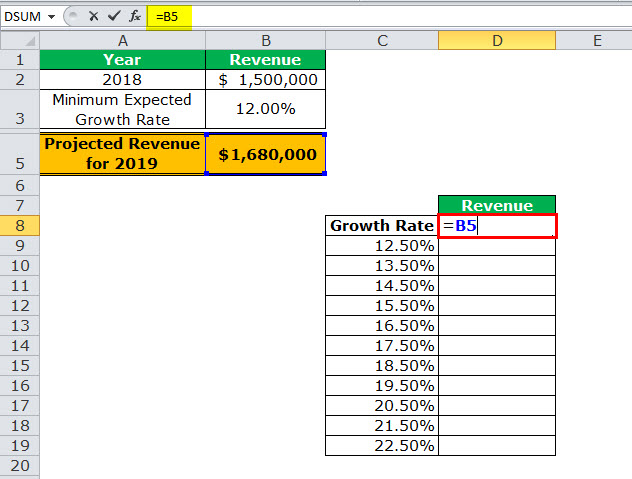
Image 1 shows an organization’s revenue (in $) for 2018 in cell B2. The minimum growth rate expected is given as 12% in cell B3. The projected revenue (in $ in cell B5) for 2019 has been calculated by using the formula “=B2+(B2*B3).”
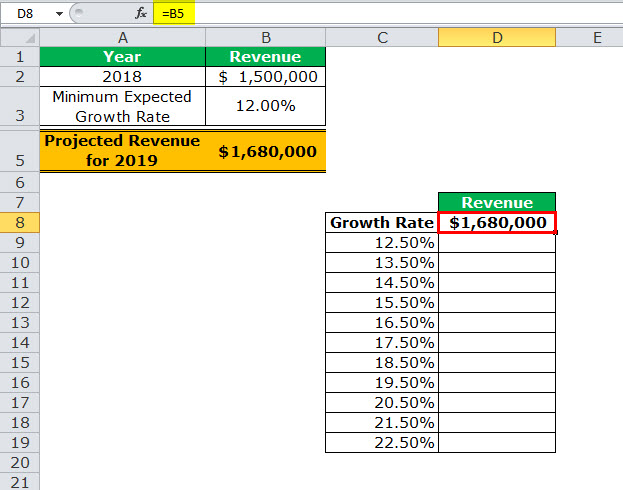
Image 2 shows the possible values (in column C) that the growth rate can assume. The value of cell D8 has been explained in steps 1 and 2 (given further in this example).

We want to perform the following tasks:

Calculate the projected revenues (in column D) according to the different growth rates (in column C) given in image 2.
Create a “line with markers” chart showing the growth rates on the x-axis and the projected revenues on the y-axis. Replace the markers of the chart with arrows.

Use a one-variable data table of Excel. Interpret the data table thus created.

Image 1

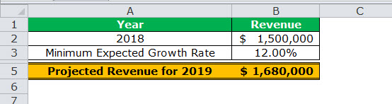
Image 2

The steps for performing the given tasks by using a one-variable data table are listed as follows:

Enter the data of the two images in Excel. In cell D8, type “equal to” (=) followed by the reference B5. This links cell D8 to cell B5.

The linking of the two cells is shown in the following image.

Since all the growth rates have been entered vertically (C9:C19), our data table is said to be column-oriented. The entire range C8:D19 is our one-variable data table. We are creating a one-variable data table as the change in outputs will be observed against a change in one input, i.e., the growth rate.

Note: Notice that either the formula “=B2+(B2*B3)” could be typed directly in cell D8 or cell D8 can be linked to cell B5. We have chosen to link the two cells.

The linking of cell D8 to cell B5 ensures that any updates in the formula of the latter are automatically reflected in the range D9:D19 of the data table. For instance, if the formula of cell B5 is multiplied by 2 [like =B2+(B2*B3)*2], all the outputs obtained in the range D9:D19 are automatically multiplied by 2.

Had we not linked cells D8 and B5, any changes to the formula of cell B5 would not have changed the value in cell D8. Consequently, the outputs in the range D9:D19 would not have been updated automatically.
Press the “Enter” key. Cell D8 shows the value of cell B5, as shown in the following image.

Notice that if one manually enters the value (1680000) in cell D8, the data table will not work. Moreover, one should always type the formula [=B2+(B2*B3)] or link the cell that is one row above and one column to the right of the possible input values (C9:C19). This is the reason we chose to link cell D8 to cell B5.

Note: If the data table is row-oriented, type the formula or link the cell that is one column to the left and one cell below the first possible input value. For instance, had the possible input values been in the range F2:P2, we would have entered the formula or linked cell E3 to cell B5.
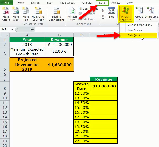
Select the range of the data table. This selection should include the linked cell (D8), the possible input values (C9:C19), and the empty cells for outputs (D9:D19). Hence, we have selected the range C8:D19, as shown in the following image.
From the Data tab, click the “what-if analysis” drop-down (in the “data tools” or “forecast” group). Select the option “data table.” This option is shown in the following image.
The “data table” dialog box opens, as shown in the following image. In the box of “column input cell,” select cell B3, which contains the minimum expected growth rate. As a result, the reference $B$3 appears in this box. Leave the box of “row input cell” blank.

By giving the reference to cell B3 in the “column input cell,” we are telling Excel that at the growth rate of 12%, the projected revenue is $1,680,000. So, with this data table, Excel is being asked the projected revenue when the growth rates vary from 12.5% to 22.5%.

Note 1: A “row input cell” or “column input cell” is a reference to a cell that contains the input. This is the input that can assume the different possible values. Moreover, this input must necessarily be used in the formula whose outputs are to be studied.

In a one-variable data table, either the “row input cell” or the “column input cell” is specified depending on whether the data table is row-oriented or column-oriented.

Note 2: In a one-variable data table, Excel uses either the formula “=TABLE(row_input_cell,)” or “=TABLE(,column_input_cell)” to calculate the different outputs. The former formula is used when the possible input values are in a row, while the latter is used when the possible input values are in a column.

To view the TABLE formula, select any of the output cells and check the formula bar. In this example, the formula “=TABLE(,B3)” is used to calculate the outputs.

Further, Excel uses these TABLE formulas as array formulasArray formulas are extremely helpful and powerful formulas that are used in Excel to execute some of the most complex calculations. There are two types of array formulas: one that returns a single result and the other that returns multiple results.read more. However, these formulas cannot be edited manually, unlike the regular array formulas. But, one can delete all the output cells containing the TABLE formulas.
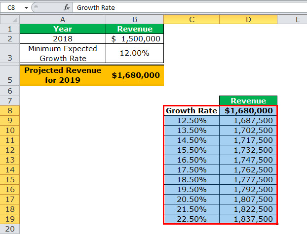
Click “Ok” in the “data table” window. The range D9:D19 of the data table has been filled with values. The different outputs are shown in the following image.

Interpretation of the one-variable data table: By looking at the data table in the preceding image, one can say that when the growth rate is 12.5%, the projected revenue is $1,687,500. Likewise, when the growth rate is 13.5%, the projected revenue is $1,702,500. Hence, the larger the growth rate, the more the increase in the projected revenue.

The projected revenue is at its maximum ($1,837,500) when the growth rate is at its highest (22.5%). So, the organization can study the variation in outputs when a single input (growth rate) changes.

Note: For more examples related to the one-variable data table of Excel, refer to the hyperlink given before step 1.
To create a “line with markers” chart that displays the growth rates on the x-axis and the projected revenues on the y-axis, follow the listed steps:

a. Select the range D9:D19 and click the Insert tab on the Excel ribbon.
b. Click the “insert line or area chart” icon from the “charts” group. Select the “line with markers” chart under the 2-D line charts. A “line with markers” chart appears, which displays the projected revenues on the y-axis.
c. Click anywhere on the chart. The “chart tools” menu becomes visible. This menu consists of the Design and Format tabs.
d. Click the Design tab of the “chart tools” menu. Choose “select data” from the “data” group. The “select data source” window opens.
e. Click “edit” under “horizontal (category) axis labels.” The “axis labels” window opens.
f. Select the range C9:C19 in the “axis label range” box. Click “Ok.” Click “Ok” again in the “select data source” window.

The “line with markers” chart is created whose x-axis and y-axis look the way they are shown in the image of step 8.
To replace the default markers of the chart with arrows, follow the listed steps:

a. Select the markers of the chart and right-click them. Choose the “format data series” option from the context menu. The “format data series” pane opens.
b. Click the “fill & line” tab. Expand the “line” tab. In “end arrow type,” select any of the arrows. We have chosen “open arrow.”
c. Select “marker” and expand the “marker options.” Choose the option “none.”
d. Close the “format data series” pane.

The “line with markers” chart looks the way it is displayed in the following image. Notice that since the chart shows the projected revenues, we have titled it accordingly.

Two-Variable Data Table in Excel

A two-variable data table in excelA two-variable data table helps analyze how two different variables impact the overall data table. In simple terms, it helps determine what effect does changing the two variables have on the result.read more helps study how changes in two inputs of a formula cause a change in the output. In a two-variable data table, there are two ranges of possible values for the two inputs. From these two ranges, one range is in a row and the other is in a column of Excel.

Example #2

There are three images titled “image 1,” “image 2,” and “image 3.” The following information is given:

Image 1 shows an organization’s revenue (in $ in 2018) and the minimum growth rate in cells B2 and B3 respectively. Both these figures are the same as that of the previous example. Additionally, the organization gives a 2% discount (in cell B4) to its customers. This is given to boost sales.
Image 2 shows how the projected revenue (in $ in cell B6) for 2019 has been calculated. The formula “=B2+(B2*B3)-(B2*B4)” is used for this purpose. The amount obtained ($1,650,000) is the projected revenue after the discount.
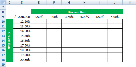
Image 3 shows the different values in row 9 that the discount rate can assume. The possible values that the growth rate can assume are given in column D. The value of cell D9 has been explained in steps 1 and 2 (given further in this example).

Calculate the projected revenues (in E10:J18) according to the various discount rates (in row 9) and growth rates (in column D). Use a two-variable data table of Excel. Interpret the data table thus created.

Image 1

Image 2

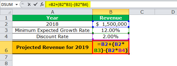
Image 3

The steps for creating a two-variable data table are listed as follows:

Step 1: Enter the data of the preceding images in Excel. In cell D9, type the “equal to” operator followed by the reference B6.

This time we have chosen to link cell D9 to cell B6. Alternatively, we could have also entered the formula [=B2+(B2*B3)-(B2*B4)] in cell D9. This is because, in a two-variable data table, one should type the formula or link the cell that is one column to the left of the first horizontal input value (2.5%). At the same time, this cell should be one row above the first vertical input value (12.5%).

The linking of cells ensures that any changes to the formula of cell B6 are reflected in the value of cell D9. Further, any change in the value of cell D9 will update the outputs (in E10:J18) automatically.

Note: Please ignore the differences in font, colors, and alignment across the images of this example. These differences may be due to the different versions of Excel being used to create the images.

Step 2: Press the “Enter” key. Cell D9 shows the value of cell B6, which is 1,650,000. This is shown in the following image.

The entire range D9:J18 is our two-variable data table. Notice that the excel data table shows the possible discount rates horizontally (in bold in row 9) and the possible growth rates vertically (in column D). This time the variation in outputs resulting from changes in both these inputs (discount rate and growth rate) need to be studied.

Note: If the value is entered manually in cell D9, the excel data table will not work.

Step 3: Select the range D9:J18. Note that the selection should include the linked cell (D9), possible discount rates (E9:J9), possible growth rates (D10:D18), and the empty cells for the outputs (E10:J18).

The selection is shown in the following image.

Step 4: Click the “what-if analysis” drop-down (in the “data tools” or “forecast” group) of the Data tab. Select the option “data table.”

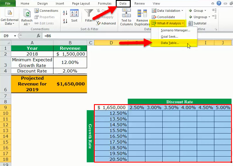
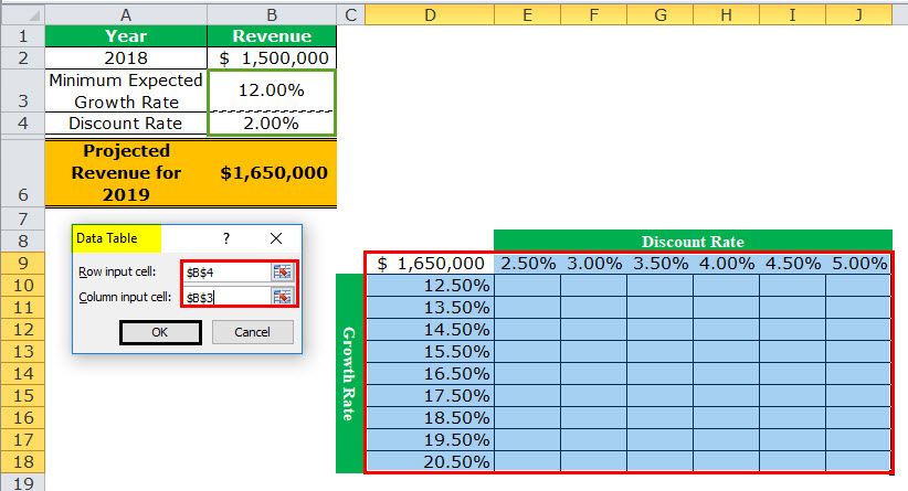
Step 5: The “data table” window opens, as shown in the following image. In the box of “row input cell,” select cell B4. In the box of “column input cell,” select cell B3. The absolute referencesAbsolute reference in excel is a type of cell reference in which the cells being referred to do not change, as they did in relative reference. By pressing f4, we can create a formula for absolute referencing.read more to cells B4 and B3 appear in the two boxes.

Cells B4 and B3 contain the minimum expected growth rate and the discount rate of the source dataset.

By making these selections, Excel is told that at a discount rate of 2% and a growth rate of 12%, the projected revenue is $1,650,000. Therefore, our two-variable data table instructs Excel to calculate the projected revenues when the discount rates and growth rates vary from 2.5% to 5% and 12.5% to 20.5% respectively.

Note: In a two-variable data table, both the “row input cell” and “column input cell” are specified, unlike a one-variable data table where one has to specify either of the two inputs.

Further a two-variable data table uses the formula “=TABLE(row_input_cell,column_input_cell)” to calculate the outputs. So, in this example, the formula “=TABLE(B4,B3)” has been used for the calculations. This formula is visible in the formula bar when an output cell is selected.

For the meaning of the “row input cell” and the “column input cell,” refer to “note 1” under step 5 of example #1.

Step 6: Click “Ok” in the “data table” window. The outputs appear in the range E10:J18, as shown in the following image.

Interpretation of the two-variable data table: When the discount rate is 2.5% and the growth rate is 12.5%, the organization’s projected revenue is $1,650,000 (in cell E10). Notice that this figure is the same as that of cell B6. However, the value in cell B6 takes into account 2% and 12% as the discount rate and growth rate respectively.

Notice that the numbers of cells E10 and B6 match those of cells G11 and I12. This implies that when the discount rate and growth rate are increased in the same proportion (like by 0.5%, 1.5% or 2.5%), the resulting value is the same as the output of the source dataset (in cell B6). Cells E10, G11, and I12 reflect 0.5%, 1.5%, and 2.5% increase in the two rates.

Likewise, had we increased both the discount and growth rates by 1%, the resulting value would have again been $1,650,000. In this case, the discount rate and growth rate would have been 3% and 13% respectively.

By obtaining the projected revenues in the range E10:J18, the organization can sell at an optimum discount rate and, at the same time, target an attainable growth rate. Hence, the organization can choose the most suitable combination of the two rates.

Note: For more examples related to the two-variable data table of Excel, click the hyperlink given before step 1 of this example.

The Key Points Governing Data Tables in Excel

The important points related to data tables of Excel are listed as follows:

It helps select those input values that fit the business in the best possible manner.
It facilitates the comparison of the different outputs as all the results are consolidated in one place.
It presents the results in a tabular format that can neither be edited nor undone with the shortcut “Ctrl+Z.” The outputs can only be deleted by selecting them and pressing the “Delete” key.
It uses the TABLE array formulas to calculate the outputs. The “row input cell” and the “column input cell” must be selected carefully to get accurate results. Moreover, the input cell or cells must be on the same worksheet as the data table.
It need not be refreshed, unlike a pivot table. A change in the values or the formula of the source dataset causes the excel data table to update automatically.

Frequently Asked Questions

1. Define a data table and suggest when it should be used in Excel.

A data table helps analyze how a change in one or two inputs of a formula causes a change in the output. The resulting outputs are arranged in a tabular format, making them easy to compare and interpret.
A data table of Excel should be used in the following situations:
• When the outputs resulting from a change in one or two inputs need to be studied
• When the most optimum input value or values need to be chosen
• When all the combinations of inputs and outputs need to be explored in one glance

2. How to create a data table in Excel?

The steps to create a data table in Excel are listed as follows:

a. Enter the source dataset in an Excel worksheet. Use one or two inputs to calculate an output.
b. Arrange the possible values, which an input can assume, in a row and/or column.
c. Link one cell of the data table to the output cell of the source dataset. Alternatively, in a cell of the data table, enter the formula whose outputs need to be studied.
d. Select the data table. The selection should include the linked cell (or the formula cell of the data table), the possible input values, and the empty cells for outputs.
e. Select the “data table” option from the “what-if analysis” drop-down of the Data tab. The “data table” window opens.
f. Enter either the “row input cell” or “column input cell” if the impact of changing one input is to be studied. To study the impact of changing two inputs, enter both “row input cell” and “column input cell.”
g. Click “Ok” in the “data table” window.

A one-variable or two-variable data table is created depending on the execution of steps “a,” “b,” and “f.”

Note: For more details on creating a data table in Excel, refer to the examples of this article.

3. How does a data table work in Excel?

A data table works on the policy “what will be the result if one or two inputs of a formula are changed?” One cell of the data table is linked to the source dataset. In this way, Excel is told how the inputs are to be used in calculating the output.

Next, as the possible input values are supplied, Excel is asked to calculate the outputs using the same formula as that of the source dataset. The resulting table shows the different mixes of inputs and outputs, thereby assisting the user in decision-making.

How to Make a Data Table in Excel: Step-by-Step Guide (2023)

Data tables in Excel are used to perform What-if Analysis on a given data set.

Using data tables, you can analyze the changes to the output value by changing the input values to a formula.

There is so much that you can do using data tables in Excel. 😀

Continue reading the article below to learn it all.

Also, download our sample workbook here to practice the examples given in this guide.

What is an Excel data table?

An Excel Data table is a What-if Analysis tool. It allows users to use different input values for a variable and assess the changes to the output value.

These are especially of help if you are operating a formula in Excel where the output depends on several variables. And you are keen to compare the results for different inputs to the formula.

Presently, Excel offers a one-variable and two-variable data table only. This means you can choose any two variable values (at max) from any formula to test.

Jump right into the article below to learn all about a data table in Excel. 🔔

How to create a one-variable data table in Excel

A one-variable data table in Excel allows users to test one variable.

For example, see the image below.

The image shows the particulars of a loan. We have three main variables in the data.

The amount of loan
The rate of interest/profit
The tenure of the loan (until it is paid back)

Example 1: Column Input Cells

In this example, let’s see keep the interest rate as the variable.

What is the yearly payment to be made against the loan?

1. Write the PMT function to find the yearly repayment against the loan.

= PMT (B3, B4, B2)

= PMT (Interest Rate, Periods of Repayment, Amount of Loan Today)

2. Multiply this number by the number of payments to be made.

That’s the total amount to be paid against the loan over 5 years.

So how much is the interest on the loan?

3. Subtract the amount of loan from the amount of repayment.

Everything’s good and sorted.

Now, what if you want to see how the repayments change if one variable (the interest rate) changes?

Do not re-perform the entire calculation all over again. The Data Table (What-if analysis) will do it for you.

4. List down the variable (interest rate in this case) that is to be changed.

5. Create a link by referring to the targeted output for each interest rate in the corresponding column.

We want Excel to give us the repayments for different interest rates. So, we have created a link to the repayment in the original calculation.

6. Select the Inputs table (the interest rates and the corresponding column for targeted output).

7. Go to Data Tab > Forecast > What-If Analysis Tools > Data Table.

This will take you to the Data Table dialog box.

8. In the Column Input Cell box, create a reference to the ‘Interest Rate’ from the original table.

Reference is made to the Interest rate because that is the variable in our data. We want to experiment with how the changing interest rates affect repayments.

We have created a reference in the Column Input Cell box and not the Row Input Cell box. This is because our Input data is in the form of a column and not a row.

Kasper Langmann, Microsoft Office Specialist

9. All set. Hit Okay and Ta-da! 😃

A one variable data table for the variable interest rates

Excel creates a one-variable data table to calculate the repayments for different interest rates.

Example 2: Row Input Cells

Let’s bring a slight variation to the above data. This time the one variable of the data is the amount of the loan.

Also, let’s change the shape of Input Data from a Column to a Row.

1. Select the Inputs Data.

2. Go to Data Tab > Forecast > What-If Analysis Tools > Data Table.

3. In the ‘Data Table’ dialog box, create a reference to the Loan amount in the Row Input Cell box.

This time the variable is the amount of the loan. We want to experiment with how the changing loan amount affects the repayments.

Must note that we have created a reference to the ‘Row Input Cell’ this time. This is because our Input Data is row-oriented.

Kasper Langmann, Microsoft Office Specialist

4. Click ‘Okay’ to see the repayment amount for differing amounts of loans.

A one variable data table for different loan amounts

What if we want to see how the total interest changes by the change in the loan amount?

Simple, refer to the amount of interest in the Inputs Data.

Changing the reference to the total interest

And there it is! Excel shows the changes to total interest instead of repayments.

How to create multiple one-variable data tables?

In the above example, what if you want to see the change in interest rates on both the repayments and total interest?

Create multiple Excel data tables. Simple.

1. In the Input Data, make two columns next to the variable interest rates.

2. In the first column, create a reference to the repayment calculation in the original data.

3. In the second column, create a reference to the total interest in the original data.

4. Create a one-variable data table by referring to the interest rate in the Column Input Cell box.

Creating a reference to the interest rate

5. Click Okay, and there you go! 🙂

Excel creates multiple one variable data table

Excel shows the result of changes in interest rates on repayments and loan amounts.

How to make a two-variable data table in Excel?

The two-variable data table is more of a two-dimensional table. It allows you to analyze how your final output changes from the changes in any two variables of your data.

Let’s continue the example above to create a two-variable data table in Excel.

This time, let’s select two variables from the data, Interest Rate, and Loan Amount. We want to see how the repayments change when both these variables change.

1. Create a two-dimensional data table with each variable on one side of the table.

In the above image, we have set the interest rates in a columnar format. Whereas the loan amount takes the shape of a row.

2. Select the intersecting cell of both the data sides.

3. In this cell, create a reference to the calculation of the repayment in the original table.

This is because we want to see how the repayments change with changes in the interest rate and the loan amount.

Our Input Data is now ready. Let’s now create a data table and perform the What-if Analysis.

4. Select the entire Data Table.

5. Go to Data Tab > Forecast > Click What-if Analysis Tools > Data table.

Accessing data table in excel from Excel ribbon

6. This opens up the data table dialog box.

7. Against the Column Input Cell box, create a reference to the interest rate from the source data.

Pay attention to how a reference is created to the interest rate against the Column Input Cell. This is because the possible input values for interest rate (the first variable) are in the shape of a column.

8. Against the ‘Row Input Cell’, create a reference to the amount of loan from the source data.

The Row Input Cell refers to the amount of the loan. This is because possible input values for the loan (second variable) are in the shape of a row.

9. Click ‘Okay’, and you’re good to go.

Woah! This seems like a very densely packed data table.

What is this? See below.

Each cell of this data table is mutual to two cells. For example, in the image above, the highlighted cell shows the amount of repayment, if the interest rate changes to 12% and the loan amount changes to 2000.

Must Note: A two-variable data table is a two-dimensional table. It captures the result of the change in any two variables at the same time.

The data table formula above is an array formula. To double-check, click on any cell from the data table and see the formula bar.

You will find the formula enclosed in curly brackets. A formula enclosed in curly brackets is an Array formula.

Kasper Langmann, Microsoft Office Specialist

Trouble Shooting the Two-Variable Data Table

The Two-Variable data table in Excel seems no less than magic. A heap of calculations is only a click away.

A two-variable data table is an array, and there is something you must know about a table array.

1. Editing a two-variable data table

Once you have created a two-variable data table, try clicking on any individual cell from the data table and making some changes to it.

You cannot make changes to a part of this data! This is all that Excel has to say in return.

A data table is an array, and you cannot make changes to individual cells of an array.

To make any changes to the data table, click the data table and select the whole of it.

1. From the formula bar, delete the Table formula.

2. Type in the desired value (let’s say 10) and hit Ctrl + Enter.

3. The entire table will be replaced by 10.

You can now make changes to any individual cells as it is no more an array.

2. Deleting a two-variable data table

Deleting two-variable data is a little science.

You cannot delete an individual value from the data table. However, you can only delete the whole data table.

Select the entire array (whole data table).
Press the delete key.
And your data table is gone.

That’s it – Now what?

Data Tables can save you big on time.

In the article above, we have learned almost all about data tables in Excel – starting from creating a single-variable data table, and multiple single-variable data tables (in one go) to creating multiple-variable data tables.

And of course, many tips.

While data tables help data analysis in Excel, you’d need many other functions of Excel to handle big data sets in Excel. The most important of these include the VLOOKUP, SUMIF, and IF functions.

Learn each of these three functions by signing up for my free 30-minute email course that teaches you these functions (and more!).

Kasper Langmann2023-01-19T12:23:16+00:00

Page load link

Источник

Excel for Microsoft 365 Excel for Microsoft 365 for Mac Excel 2021 Excel 2021 for Mac Excel 2019 Excel 2019 for Mac Excel 2016 Excel 2016 for Mac Excel 2013 Excel 2010 Excel 2007 More…Less

To make managing and analyzing a group of related data easier, you can turn a range of cells into an Excel table (previously known as an Excel list).

Note: Excel tables should not be confused with the data tables that are part of a suite of what-if analysis commands. For more information about data tables, see Calculate multiple results with a data table.

Learn about the elements of an Excel table

A table can include the following elements:

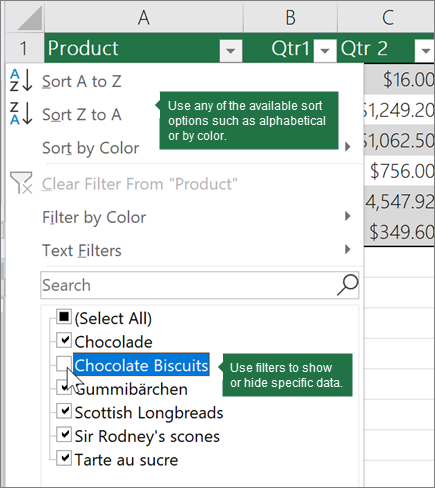
Header row By default, a table has a header row. Every table column has filtering enabled in the header row so that you can filter or sort your table data quickly. For more information, see Filter data or Sort data.

You can turn off the header row in a table. For more information, see Turn Excel table headers on or off.
Banded rows Alternate shading or banding in rows helps to better distinguish the data.
Calculated columns By entering a formula in one cell in a table column, you can create a calculated column in which that formula is instantly applied to all other cells in that table column. For more information, see Use calculated columns in an Excel table.
Total row Once you add a total row to a table, Excel gives you an AutoSum drop-down list to select from functions such as SUM, AVERAGE, and so on. When you select one of these options, the table will automatically convert them to a SUBTOTAL function, which will ignore rows that have been hidden with a filter by default. If you want to include hidden rows in your calculations, you can change the SUBTOTAL function arguments.

For more information, also see Total the data in an Excel table.
Sizing handle A sizing handle in the lower-right corner of the table allows you to drag the table to the size that you want.

For other ways to resize a table, see Resize a table by adding rows and columns.

Create a table

You can create as many tables as you want in a spreadsheet.

To quickly create a table in Excel, do the following:

Select the cell or the range in the data.
Select Home > Format as Table.
Pick a table style.
In the Format as Table dialog box, select the checkbox next to My table as headers if you want the first row of the range to be the header row, and then click OK.

Also watch a video on creating a table in Excel.

Working efficiently with your table data

Excel has some features that enable you to work efficiently with your table data:

Using structured references Instead of using cell references, such as A1 and R1C1, you can use structured references that reference table names in a formula. For more information, see Using structured references with Excel tables.
Ensuring data integrity You can use the built-in data validation feature in Excel. For example, you may choose to allow only numbers or dates in a column of a table. For more information on how to ensure data integrity, see Apply data validation to cells.

Export an Excel table to a SharePoint site

If you have authoring access to a SharePoint site, you can use it to export an Excel table to a SharePoint list. This way other people can view, edit, and update the table data in the SharePoint list. You can create a one-way connection to the SharePoint list so that you can refresh the table data on the worksheet to incorporate changes that are made to the data in the SharePoint list. For more information, see Export an Excel table to SharePoint.

Need more help?

You can always ask an expert in the Excel Tech Community or get support in the Answers community.

Data Table in Excel

Data tables are used to analyze the changes seen in your final result when certain variables are changed from your function or formula. Data tables are one of the existing parts of What-If analysis tools, which allow you to observe your result by experimenting it with different values of variables and to compare the outcomes stored by the data table.

There are two types of a data table, which are as follows:

One-Variable Data Table.
Two-Variable Data Table.

How to Create Data Table in Excel?

Data Table in Excel is very simple and easy to create. Let’s understand the working of the Data Table in Excel by Some Examples.

You can download this Data Table Excel Template here – Data Table Excel Template

Data Table in Excel Example #1 – One-Variable Data Table

One-variable data tables are efficient in the case of analyzing the changes in the result of your formula when you change the values for a single input variable.

Use case of One-Variable Data Table in Excel:

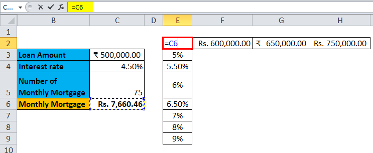
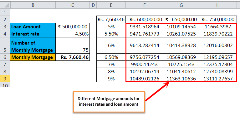
The one-variable data table is useful in scenarios where a person can observe how different interest rates change the amount of their mortgage amount to be paid. Consider the below figure, which shows the mortgage amount calculated based on the interest rate using the PMT function.

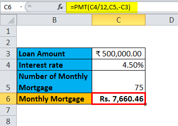
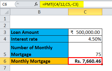
The table above shows the data where the mortgage amount is calculated based on the interest rate, mortgage period and loan amount. It uses the PMT formula to calculate the monthly mortgage amount, which can be written as =PMT (C4/12, C5,-C3).

In the case of observing the monthly mortgage amount for different interest rates, where the interest rate is considered as a variable. In order to do this, there is a need for creating a one-variable data table. The steps to create the one-variable data table are as follows:

Step 1: Prepare a column which consists of different values for the interest rates. We have entered different values for interest rates in the column which is highlighted in the figure.

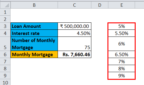
Step 2: In the cell (F2), which is one row above and diagonal to the column which you prepared in the previous step, type this = C6.

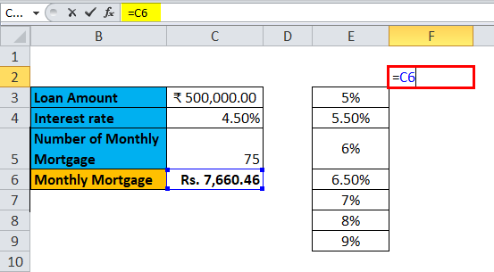
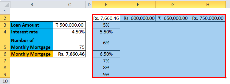
Step 3: Select the entire prepared column by values of different interest rates along with the cell where you had inserted the value, i.e. F2 cell.

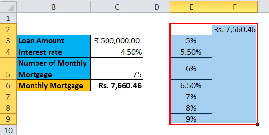
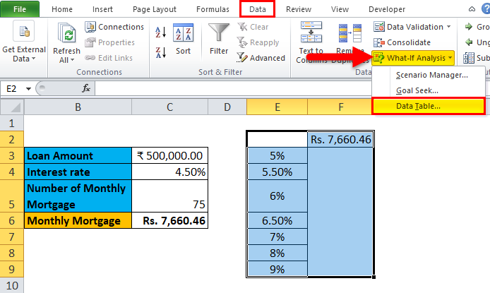
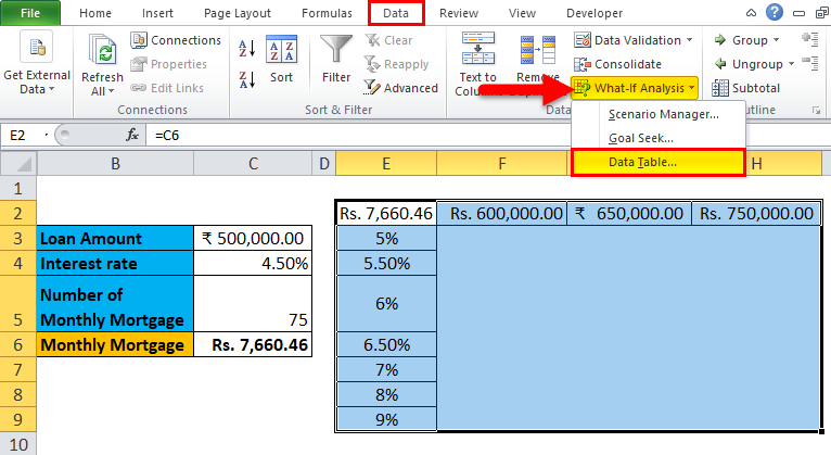
Step 4: Click on the ‘Data’ tab and select ‘What-If Analysis’, and from the options popped down, select ‘Data Table’.

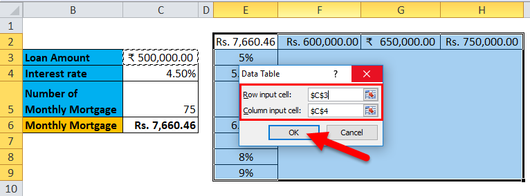
Step 5: Data table dialog box will appear.

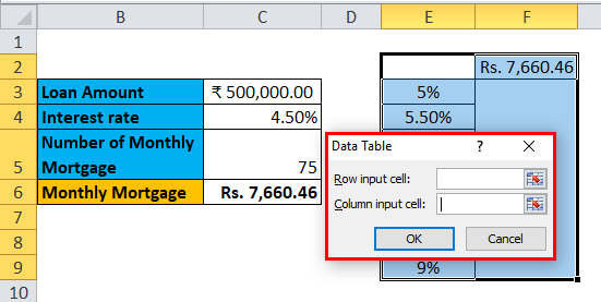
Step 6: In the Column input cell, refer to cell C4 and click OK.

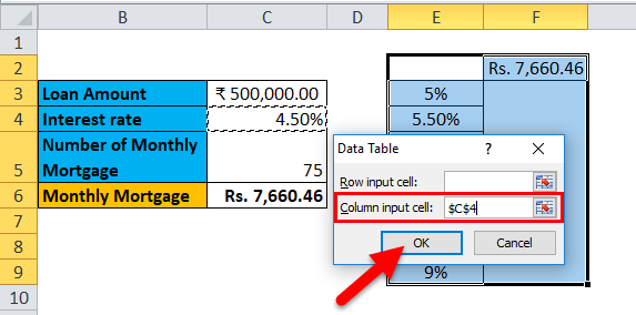
In the dialog box, we refer to the cell C4 in the Column input cell and keep the row input cell empty as we are preparing a data table with one variable.

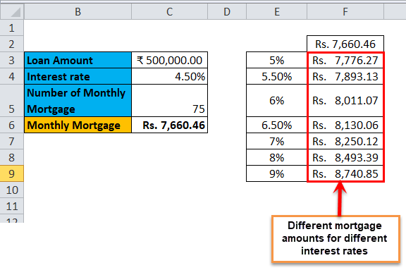
Step 7: After following all the steps, we get all the different mortgage amounts for all entered interests rates in column E (unmarked), and the different mortgage amounts are observed in column F (marked).

Data Table in Excel Example #2 – Two-Variable Data Table

Two-variable data tables are useful in scenarios where a user needs to observe the changes in the result of their formula when they change two input variables simultaneously.

Use-case of Two-Variable Data Table in Excel:

The two-variable data table is useful in scenarios where a person can observe how different interest rates and loan amounts change the amount of their mortgage amount to be paid. Instead of calculating for individual values separately, we can observe them with instantaneous results. Consider the below figure, which shows the mortgage amount calculated based on the interest rate using the PMT function.

The above example is similar to our example shown in the previous case for a one-variable data table. Here the mortgage amount in cell C6 is calculated based on the interest rate, mortgage period and loan amount. It uses the PMT formula to calculate the monthly mortgage amount, which can be written as =PMT (C4/12, C5,-C3).

In order to explain the two-variable data table with reference to the above example, we will show the different mortgage amounts and choose the best which suits you by observing the different values of interest rates and loan amount. In order to do this, there is a need for creating a two-variable data table. The steps to create the one-variable data table are as follows:

Step 1: Prepare a column which consists of different values for the interest rates and loan amount.

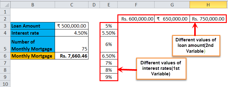
We have prepared a column consisting of the different interest rates, and in the cell diagonal to starting cell of the column, we have entered the different values of the loan amount.

Step 2: In the cell (E2), which is one row above to the column which you prepared in the previous step, type this = C6.

Step 3: Select the entire prepared column by values of different interest rates along with the cell where you had inserted the value, i.e. E2 cell.

Step 4: Click on the ‘Data’ tab and select ‘What-If Analysis’, and from the options popped down, select ‘Data Table’.

Step 5: A Data table dialog box will appear. The ‘Column input cell’ refers to cell C4 and in the ‘Row input cell’ C3. Both the values are selected as we are changing both the variables and Click OK.

Step 6: After following all the steps, we get different values of mortgage amounts for different values of interest rates and loan amount.

Things to Remember About Data Table in Excel

For one variable data table, the ‘Row input cell’ is left empty, and in a two-variable data table, both ‘Row input cell’ and ‘Column input cell’ are filled.
Once the What-If analysis is performed, and the values are calculated, you cannot change or modify any cell from the set of values.

What are Data Tables?

Data tables are used in Excel to display a range of outputs given a range of different inputs. They are commonly used in financial modeling and analysis to assess a range of different possibilities for a company, given uncertainty about what will happen in the future.

How to Create Excel Data Tables

Below is a step-by-step guide on how to create an Excel data table. In the example, we will look at how much operating profit a company will generate based on different product prices and different sales volumes. We have built a simple model that assumes one variable cost (cost of goods sold), and one fixed cost (general and administrative expenses).

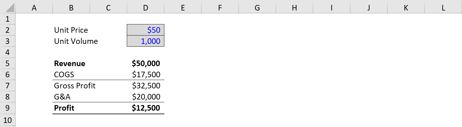
Step 1: Create a Model

The first step when creating data tables is to have a model in place. We’ve made a simple model that includes two key assumptions: unit price and unit volume. From there, we have a simple income statement that includes revenue, COGS, G&A, and operating profit (EBIT).

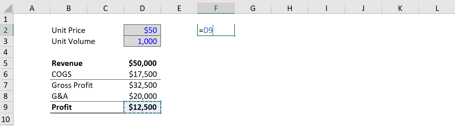
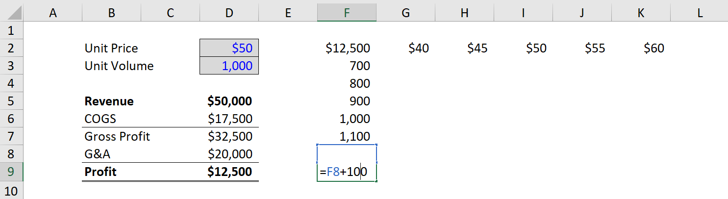
Step 2: Link the Output

Since profit is what we want to use as the output, we simply take an empty cell in the model and link it to net income at the start of the data table (the top left corner).

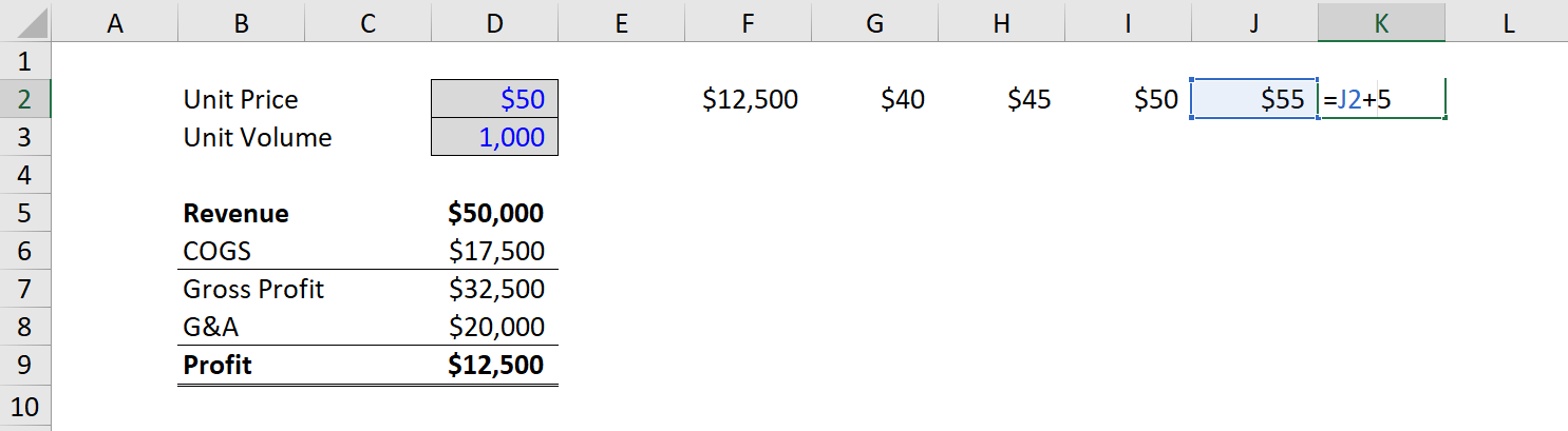
Step 3: Enter the Input Values

Once net income is linked, we need to enter the different values we want to test for unit prices and unit volumes. To do it, we manually enter the values across the top and left sides of the table. In this case, we will enter unit prices from $40 to $60 and volumes from 700 to 1,300.

To learn more about how to perform this type of analysis, check out CFI’s Sensitivity Analysis Course.

Step 4: Highlight the Cells and Access the Data Tables Function

With the structure of the table complete, the next step is to highlight all the cells with data that will be used to form the table, and then access the Excel data tables function under the Data ribbon and What-If analysis.

The keyboard shortcut on Windows is Alt, A, W, T.

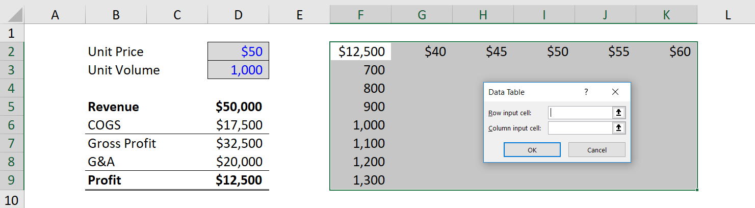
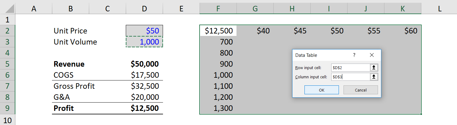
Step 5: Link the Input Values

This can be one of the trickiest steps when setting up data tables. Financial analysts often aren’t sure where the Row Input Cell goes and where the Column Input Cell goes. The easiest way to think about it that the Row refers to the assumptions across the top of the table, and the Column refers to the assumptions across the left of the table. So, link each of them to the hard-coded assumptions that drive the model.

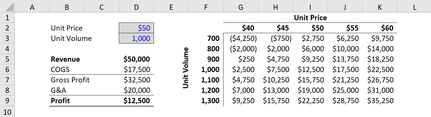
Step 6: Format the Data Table Output

Once the table is linked, it can be helpful to do some basic formatting so that the data table is easier to read. This includes adding borders and labels, so users can easily see the information contained in the analysis.

You can download the Excel file for the example we worked through together in this guide. Use it to perform your own analysis!

Download the Free Data Table template here.

Applications in Sensitivity Analysis

The main application of data tables is in performing sensitivity analysis for financial modeling and valuation. Since financial models represent a best-guess scenario on what the future holds for a business, it can be helpful to see how sensitive the value of the business is relative to various changes in assumptions.

To learn more about how to perform this type of analysis, check out CFI’s Sensitivity Analysis Course.

Additional Resources

Thank you for reading CFI’s guide to data tables, what they are, how to build them, and why they matter. To learn more and continue advancing your career, these additional CFI resources will be helpful:

Analysis of Financial Statements
Best Practices in Financial Modeling
How to Link the 3 Financial Statements
Scenario Analysis
See all Excel resources

Источник

Excel table is a series of rows and columns with related data that is managed independently. Excel tables, (known as lists in Excel 2003) is a very powerful and super-cool feature that you must learn if your work involves handling tables of data.

What is an Excel table?

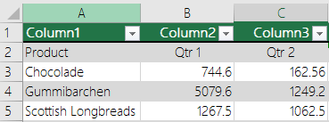
Table is your way of telling excel, “look, all this data from A1 to E25 is related. The row 1 has table headers. Right now we just have 24 rows of data. But I can add more later!”

When you make a table (more on this in a sec) you can easily add more rows to it without worrying about updating formula references, formatting options, filter settings etc. Excel will take care of everything thus making you a data guru.

How to create table from a bunch of data?

To create an excel table, all you have to do is select a range of cells and press the table button from Insert ribbon in Excel (or use the shortcut CTRL+T).

See this simple tutorial:

Today we will learn 10 excel data table tricks that will make you a data guru, no let’s make that DATA GURU.

The most important thing after you create a table – Give it a name

Once you have a table, go to design ribbon and give your table a name. If you don’t name it, Excel will call it Table2 or whatever. But once you name it, you can write meaningful formulas thru sweet sweet structural references feature. So name your tables.

1. Change table formatting without lifting a finger

Excel has some great predefined table formatting options. Just select any cell in your table and change the table formatting by going to “format as table” button in the home ribbon.

If you are bored with the predefined formats, you can easily define your own table formatting color schemes and apply them.

2. Add Zebra Lines to Tables without doing Donkey Work

When you create a table, zebra lines come as a bonus. And when you add new rows to the table, excel takes care of zebra lining or banding automatically. You can turn on / off the banded rows feature from “design ribbon tab” as well.

That means you don’t need to use conditional formatting or manually format alternative rows in different color.

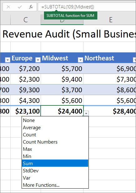
3. Tables come with Data Filters and Sort Options by default

Each data table comes with filters and sorting options so that you can filter and sort the data in that table independently. That also means, if a worksheet has 2 tables, they each get their own data filters (usually excel wont allow you to add more than one set of filters per sheet, but when it comes to tables, all exceptions are made, just for you)

4. You can also Slice your tables with slicers

That is right. When you have a table of data, you can insert a slicer (either from design ribbon or insert ribbon) and use that to filter your table data intuitively.

Learn all about Excel Slicers.

5. Bye, bye cell references, welcome structured references

The most important advantage of tables is that, you can write meaningful looking formulas instead of using cell references. When you create and name the table (you can name the table from design tab), you can write formulas that look like this:

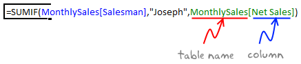
The beauty of structured references is that, when you add or remove rows, you don’t need to worry about updating the references.

Learn all about structural references in Excel.

6. Make Calculated Columns with ease

Any tabular data will have its share of calculated columns. Excel tables make having calculated columns very easy. With structured references, all you need to know is English to make a calculated column. The beauty of calculated columns in table is that, when you write formula in one cell, excel automatically fills the formula in the rest of cells in that column. That would make you an instant data guru.

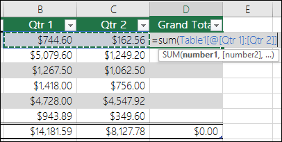
7. Total your Tables without writing one formula

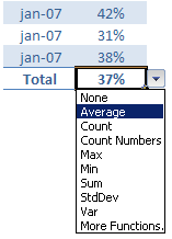
The ability to summarize data with pivot tables is extended to excel tables as well. You can add total row to your table with just a click.

What more, you can easily change the summary type from “sum” to say “average”.

8. Convert table back to a range, if you ever need to

If you ever wanted to go back to a normal range of data, you can easily convert the tables back to named ranges.

Excel will take care of the formulas and change the references to cell references.

9. Export Tables to Pivot Tables, Woohoo

What good is a bunch of data when you can’t analyze it? That is where Pivot tables come in to picture [pivot table tutorial]. Thankfully, you don’t need to do much. Just click a button and your table goes to pivot table.

10. Push the table data to Sharepoint Intranet Site

If you have a corporate intranet Sharepoint portal, you can easily publish the excel tables as share-point lists. This can be handy if you want to publish, say the top 10 sales persons of the quarter on the intranet.

11. Print Tables Alone, with out all the other stuff around

Select the table, hit CTRL+P and in settings area, select “Print Selected Table” option to print your beautifully formatted Excel table.

12. Change, reshape or clean your table data with Power Query

When you have data in a table, you can easily load it to Power Query (Get & Transform Data) using the “From Table” button.

Here is an an example of what Power Query can do for you.

13. Got multiple tables? Connect them to make a multi-table pivot

When you have more than one table, you can also connect them using Excel’s relationship feature. This way, you can build multi-table pivots to create powerful analysis of your data.

Learn all about Excel Table Relationships.

So, What do you think about Excel tables?

I say, give them a try. They have been around for more than a decade, but I still see people not using them. Setting up your data as a table is the easiest and most awesome thing you can do it. You can find some cool uses for tables in your day to day work. They are intuitive, easy to use and provide great power without added complexity.

Related Material

Beginner:
- Using Structural References with Tables
- Connecting multiple tables
- Writing lookups or other formulas on tables
Advanced:
- Relative referencing in Tables
- Sum & Count filtered values in Tables
- Custom table styles to get weekend weekday zebra lines
More sources about tables:
- Create a table in Excel – Video Tutorial
- 23 things to know about Excel Tables
- Customizing table features (turn-off auto formula fill down etc.)

Share this tip with your colleagues

Excel and Power BI tips - Chandoo.org Newsletter

Get FREE Excel + Power BI Tips

Simple, fun and useful emails, once per week.

Learn & be awesome.

132 Comments
Ask a question or say something…
Tagged under

Analytics, data, data filters, Excel 101, excel tables, formatting, list posts, Microsoft Excel Conditional Formatting, Microsoft Excel Formulas, pivot tables, printing, references, screencasts, sharepoint, sorting, structured references, tables, tutorials
Category:

Excel Howtos, Featured, Learn Excel

Welcome to Chandoo.org

Thank you so much for visiting. My aim is to make you awesome in Excel & Power BI. I do this by sharing videos, tips, examples and downloads on this website. There are more than 1,000 pages with all things Excel, Power BI, Dashboards & VBA here. Go ahead and spend few minutes to be AWESOME.

Read my story • FREE Excel tips book

Excel School made me great at work.

 5/5

Excel formula list - 100+ examples and howto guide for you

From simple to complex, there is a formula for every occasion. Check out the list now.

Calendars, invoices, trackers and much more. All free, fun and fantastic.

Power Query, Data model, DAX, Filters, Slicers, Conditional formats and beautiful charts. It’s all here.

Still on fence about Power BI? In this getting started guide, learn what is Power BI, how to get it and how to create your first report from scratch.

Related Tips

132 Responses to “Excel Tables Tutorial & 13 Tips for making you a Data Guru”

Peter H says:

Chandoo, I have only been using data tables for a few weeks & have discovered that they can be used to have charts dynamically expand to take in new data.
Simply set up the chart data in a block with appropriate headings (headings must be text, not formula).
Convert it into a table, select the whole table and insert a chart.
Format the chart as required.
When new data is added the the table and chart will expand to show the data.
The only problem I have found is that the last column of data must show a number when inserting the chart- a blank, #N/A and perhaps text will cause wierd changes in the chart. However this only occurs when first inserting the chart once set up it accomodtes blanks & #N/A etc. This is easily over by adding a temporary number when required on setting up the chart then replacing it with the correct formula when the chart is complete.
This seems to be a lot easier than using offset formula for the series .
Nice post. I’ve been using Pivot Tables for years but haven’t used the «table» button until now.
Michelle says:

This is great! Never used data tables before but it helps a lot. One question though, if I try drag your SUMIF formula across a row, different columns are selected in the formula. Normally you can make the columns static in a formula by using «$» — any suggestions on doing the same here?
- Leah says:
  
  Convert the data to range. Enter your SUMIF formula, then convert it back to a table.
  - Richard says:
    
    This doesn’t work….well, it only worked one way when I tried it. I had the data as a table and had created some SUMIFS formulae on another sheet. I coverted the data table to range and the formulae all changed to use range references. But when I changed the data back to table, the formulae stayed the same.
- David N says:
  
  Creating absolute structured references is a bit awkward but not difficult.
  
  Some Column as a relative reference
  =SUM(Table1[Some Column])
  
  Some Column as an absolute reference — repeat the column name
  =SUM(Table1[[Some Column]:[Some Column]])
  
  The Some Column cell of the current row as absolute — repeat the column name — with the Other Column cell of that same row as relative
  =SUM(Table1[@[Some Column]:[Some Column]],[@Other Column])
  
  The range of Some Column to Other Column as entirely relative — repeat the table name
  =SUM(Table1[Some Column]:Table1[Other Column])
Nice post. Nice to see such useful options in 2007.
Frederick says:

hi Chandoo,

How do you «record» the screen captures of the screens that you need to show into the animated gifs? Do you use a special software for it?
- Erin says:
  
  Use the snipping tool on the start menu.
  - Earl says:
    
    You’re posting 4 years late… and I’m posting 5 years late…. 🙂
- I use Camtasia to record and produce these animated gifs. You can get a trial version here: techsmith.com
Thank you. This is truly a gem that will save hours and hours of time.
Robbert says:

Nice post! However, in a basic form this functionality already existed in Excel 2003 as a ‘List’ (ctrl-L). So it not needed to convert the table back to a normal range for excel 2003 users.
Michael says:

Chandoo,
nice post. Seems to be a useful feature. Does data tables exist in Excel2003 as well?
@Peter H: Very cool tip about the charts and data tables.

@Dan: Tables are very useful and simple. Pivot can be very powerful for data analysis, but tables are good for maintaining databases.

@Michelle: The sumif formula in the article is written outside the table in a cell. If you write formulas in and copy (ctrl+c) and paste them, then the references are not changed. But if you drag the cell (thus auto-fill), then the cell references to table columns are changing. Not sure why excel would behave like this.

Also, inside the table, you can use [#this row] operator to calculate values for that row alone.

@Frederick: I use camtasia studio to record the screen. It is a nice software. You can test it from techsmith website.

@Doug: You are welcome 🙂

@Robert: My mistake, I meant version earlier than excel 2003.

@Michael: yeah, they are called as Lists. Press, Ctrl+L to create one.
[…] since I have learned the tables feature in Excel 2007, I have fallen in love with that. They are so awesome and so user […]
bazlina says:

i kept saying OMG WOW THATS AMAZING over and over.
i’m quite new with excel so your blog helps a lot and this post, is truly great. thank you!
[…] Microsoft Excel Table Tips and Tricks – Learn Data Tables and Become a Data God | Pointy Haire…By chandoo.org October 16, 2009- ???????Excel???????????????……?X?…… […]
[…] Microsoft Excel Table Tips and Tricks – Learn Data Tables and Become a Data God | Pointy Haire…By chandoo.org October 16, 2009- ???????Excel???????????????……?X?…… […]
[…] Microsoft Excel Table Tips and Tricks – Learn Data Tables and Become a Data God | Pointy Haire…By chandoo.org October 16, 2009 […]
g7 says:

4. Bye, bye cell references, welcome structured references

it does not beat absolute reference to cell i.e $A$1, because if named range is used, it will not copy correctly if u use cell dragging horizontally… it will move to the next name range
- Joe Blauh says:
  
  This is a huge negative for «structured» references. Excel created a nifty tool that requires me to accept a significant loss of functionality if I decide to use it. It also prohibits dragging cell references to change formulae, so if I drag to fill, I have to click into the cell to manually edit the reference cells to what they should be instead of being able to drag the cell reference box back to the correct column. A small step forward and a giant step back. Or, more succinctly, Microsoft — ‘nuf said.
  - Mark F. says:
    
    Thanks for the information. Disappointing answer but helps solve my problem.
sb says:

Chandoo,

I have a question on this. In my sheet I have the «Total Row» added. In that I take an average of a column values and I need to reference this final Average value elsewhere. How Can I reference this specific «totalled average cell» such that when new rows are added the same cell is taken?

As of now, since the total is at the bottom of the table, when a new row is added the cell id of this «total average» row keeps changing. I tried to move it to the top of the table to keep it constant but I couldn’t.

thank you
sb
@SB.. you can use the [#totals] tag in the structured reference to total row else where like this:

=Table1[[#Totals],[Column1]] This will work even when you add more rows to the table.
- Siddhant Gupta says:
  
  Hi Chandoo,
  when i use this code it always shows a #Ref! error.Can you please help me to fix it?
  Thanks!
  Siddhant
sb says:

Thanks @chandoo.
[…] will save precious amount of time when you are busy modeling. (100s of tips on keyboard shortcuts, excel tables, formulas, charting & […]
[…] Select your list of products (or invoices or cats) and make it in to a table. (here is a helpful tutorial on excel tables). […]
[…] Simplifying data analysis with Excel Tables […]
V S Venkatraman says:

Dear Chandoo (Excel Guru)

Thank you very much for sharing such useful tips… now I feel more confident in analyzing a data with Excel….

Regards
Chandoo,

Where referecing table columns as range input to formulas such as sumif(), is it possible to get Excel to treat the reference as static for «fill» purposes?

Cheers,

Steve
@DangerMouse.. you can use ctrl+c ctrl+v instead of drag fill technique to treat the table references as static.
olegko says:

How to make absolute reference on Table column?
I have Table1 and use such formula:
=SUMIFS(Table1[Pay],Table1[Month],G9)

I want to “freeze” columns “Table1[Pay]” and “Table1[Pay]” in formula (like $A:$A).
How to do it?
Chris says:

Looking at article like these make me sad 🙁 — still being laden with 2003 really goads when you see so many fantastic improvements just out of ones rech like this……
[…] Excel Tables, a newly introduced feature in Excel 2007 is a very powerful way to manage & work with tabular data. I really like tables feature and use it quite often. If you are new to tables, read up Introduction to Excel Tables. […]
Avinash Ahire says:

I want to learn some excel course from you.
If you have any training centre in Mumbai, Please let me know..
Excellent Work!

Thanks
Avinash Ahire
- javed sheikh says:
  
  i want to learn some advance tally course from you
  if you have a training center in mumbai any location, please let me know
  Excellent work!
[…] 10 Tips on using Excel Tables […]
5.antiago says:

Is there a better way than ctrl-c-ctrl-v to expand the ~ifs() formulae across a row while keeping the absolute references to the auto-named ranges in the data-table? I know this has been mentioned a few times in the comments but I’m hoping someone cleverer than me might re-look at this…

All I’ve got so far is transposing my new table I’m trying to create so I’m dragging down instead of across, which holds the named column references, but I would prefer a dragging across solution

This is my first post on your website Chandoo, but I’ve been reading for a couple of weeks. It’s a fantastic site! Thanks for all your efforts
brices11 says:

I love it, I love it, I love it. Don’t know how many errors I run into because of bad cell references this should help mitigate this.
PM says:

Ok REALLY stupid question, I created the table and I have been putting in formulas using the column names, how do I «without using my mouse» select the table name from the tool tip ( or drop down) that shows up. Currently I have to scroll my mouse down to the right column name and then click it add the bracket etc. This also applies for when I use formulas in general. Please help, I am trying to be «Mouse free» 🙂

I have been using Excel forever this is amazing.
Jim Morley says:

Hi Chandoo,

I am using Excel 2007.

I am using an excel workbook to enter data for several different sites (each site has its own worksheet). I want to establish a summary worksheet showing the consolidated data accross all sites so as I enter data into the individual site worksheets the data is also replicated in the summary worksheet which is then sorted by site to show the consolidated view of all sites. Each of the site worksheets have the same data headings which will be replicated in the summary worksheet.
Can you please give me some advice as to how I can go about this?

I know how to use the basics of excel but know nothing about using databases like Access so I would prefer to continue to gather the information in excel if this can be done.

Hoping you can help me,

Jim Morley
[…] The Data Table function should not be confused with the Insert Table function. […]
[…] Excel 2007, Microsoft has introduced a powerful and useful feature called as Tables. One of the advantages of Tables is that you can write legible formulas by using structural […]
padmanarayanan says:

Chandoo,
I really missed you discount offer last week or so,That day i could not access the internet.Any chance of getting discount offer, i am really interested in joining your course.pl let me know.
Jen says:

Chandoo, thanks a lot for all your tips and tutorials. Your tutorials are really great and easy to follow!!!
Hi, Can i access Excel 2007 table via code — JavaScript?
Jonathan says:

WOW!
I’ve spent days organising a «table» of my own (without knowing it) writing formulas,creating helper columns and generally getting stuck and i just figured out that tables and pivot tables do all this in minutes. I dont know whether to feel downhearted or elated that i’ve learnt this! (all be it too late)
[…] Learn Conditional Formatting 3. Making Dashboards using Excel 4. Project Management with Excel 5. Working with Excel Tables Topics & Archives 1. Learn Excel — Topic-wise 2. Charting Tips, Tricks and Tutorials 3. Ask an […]
Debaranjan samal says:

Hi ,

I need a vba for excel training in delhi, kindly suggest regarding this..
Deb says:

How do I get the AutoFormat of Double-Bars in XL 2010? It was so easy in 2003, but I cannot find a way to do it, w/o VBA, in 2010! It can’t be that hard.

In 2003, Format, AutoFormat, choose the List 2 style. It formatted rows in groups of twos, or pairs. Very handy in lots of cases.

Any ideas?

Thanks
[…] Learn more about Excel Tables. […]
[…] How to Use Tables to Speed up Formatting of your Data […]
Premalatha says:

I have become a fan of tables now. 🙂
Premalatha says:

Hi Chandoo,

I used structured reference but when I close and open again, they have all become cell references! Is there a way to fix this? I am using 2010. Thanks,
Prem
- Prasad says:
  
  Even I have the same problem and worst is it when we add new rows the formulas now do not get changed as it is now having cell references 🙁
  
  Regads,
  Prasad DN
  - JonERotn says:
    
    Make sure you’re saving in the 2007 or 2010 format (instead of the 93/97 format).
Muhammad Bilal Yousaf says:

Dear Sir,
i want tech the micro soft excel data table and function for opperating the micro soft excel. please give send the tip of micro soft excel.

with best regards and wishes,

Muhammad Bilal Yousaf
FarooqAsim says:

Dear
I went to some new learn work in excel
latest
best Regard
Farooq Asim
Linda says:

Absolute references:
As Chandoo says, these move if you use drop and drag. However, if you highlight the required cells, place the cursor in the cell to be copied and use Ctl Enter then the formula copies keeping the references «absolut»

Linda
[…] have set up this data in an Excel Table called as tblSales so that it is easier to write […]
Eric says:

I’ve tried to name tables so that I can reference them in functions, etc… but I’m not having any luck getting the name to stick. I can click in the area to the left of the function button and type a new name for the table, but clicking outside of that causes the name to revert back to what it was (for instance, 386, or 3). Thoughts?
- @Eric
  
  Select any cell in the Table you want to rename
  
  You should see a Table Tools, Design Ribbon
  
  Select that Ribbon and on the Left there is a Table Name: dialog
  
  Change the name and press Enter
[…] wrote a great post several years ago that explained the basics of Excel tables and provided a number of tips and tricks related to them. […]
Naresh Koganti says:

How to rename a Data Table name in Excel.
- Naresh Koganti says:
  
  Sorry guys i got it.
vimal says:

i like you your website, but i quesestion i wil written to excel in accountant but evry time name party not incuding, so anything i find to party name is all ready this excel in ready name ,so you my question solve and reply to me my email id vimal_jariwala15@yahoo.ca
Nitin K. says:

Hi,

How can one add zebra lines in table rows in Office 2010?
- @Nitin K.
  When you say Table I assume you have a Table setup using the Insert Table menu
  If so goto the Table Tools, Design Tab
  Select one of the Zebra styles or edit one to setup your own colors
  If you don’t have a Data Table, select your Data and goto Insert, table menu, then follow the instructions above
  You may also want to have a read of: http://chandoo.org/wp/2011/12/08/formula-forensics-no-005/
Paul Nickell says:

I have learned so much in the last few weeks since joining in here. Well done.
Now I have a query that I need hlep with. The company I have started working for uses loads of data. Reports are exported to Excel then sorted etc etc…
The Key ref numbers are numeric, 12345.1 and 12345.10 etc etc. Excel will obviously sort the .10 above the .1 — Its an habbit of the reporting software to create a .1 and not .01 Is there anyway within Excel to block alter all the .1’s to .01’s? I’m talking thousands of them, not just a handful that could be formated as text manually.
[…] Use Excel Tables: Since Excel 2007, we can create tables from structured data and write formulas, create charts that refer to dynamic ranges with ease. Click here to know more about tables. […]
[…] the dashboard on the Property Register converted to an Excel Table (a 2007+ feature that many are still unaware of) enables the use of Slicer selectors in Excel 2013 to quickly give a dashboard feel. It’s […]
Steve Jones says:

Great site, and your instructions are so easy to follow. Thanks so much!
On sheet 1, I have a table of names and demographic information for each.
On sheet 2, I am using the same table of names but different data across the columns.
When I add a New Name to the table on Sheet 1, I have to manually extend the table on Sheet 2, to expose the new name.
Is there a way to automatically expand the table on sheet 2, to show the new name added to the table on Sheet 1??
Thanks so much
Paddy says:

Has anyone tried using named tables as data sources outside of Excel? For instance, referencing the table for a mail merge? If so, how have you got it to work? Thank you all!
- Colleen says:
  
  Yes. I use tables in a mail merge. There’s no trick (I can think of) to it different than using any other Excel data to mail merge. My own notes for mail merging mention that I open the Excel spreadsheet first and that I need to make sure that the active sheet is the sheet with the table I want to use on it. I do seem to have had problems if a different sheet is the active one.
  
  There IS a trick to making sure your Excel formatting (like number formatting for $, etc.) comes through. But that is true whether or not you are using a table.
[…] of data in this dashboard is captured using Excel Tables. This has several […]
Colleen says:

I like to say, «If you’re not using tables, you’re doing it wrong.» Or at least 90% of the time you should be using them!

I would like to say, «Tables are the best thing since sliced bread», but it then occurs to me that sliced bread is highly overrated. I can slice my own loaf much quicker than doing many of the things manually in Excel that tables make easier.

I LOVE tables! They have changed how quickly and awesomely I can analyze and present data.
Gijs says:

Hi Chandoo, another awsome tutorial.

Can you expand the VBA so that i can leave some categories blank and the table will show ALL entries for that category? (eg all Customer Types or all Regions)?

Thanx, Gijs.
[…] ourSales[month] refers to the month column in the ourSales table. Works only in Excel 2007 or above. Know more about Excel Tables. […]
Chandra says:

So I created a data table and wrote forumlas using the data table and column names. It all calculated out beautifully. HOWEVER, now that I want to add lines to my data table, none of the formulas are seeing the added data. I’ve gone in to expand the range of the table, etc. But still no luck. So stinkin’ frustrated :/ Any advice??
[…] best way to create a tracker is to use Excel tables. Set up one with 4 columns – Employee name, vacation type, start date & end date, like […]
Reena says:

Hi,
I need to convert some data into columns can anyone help me?
[…] Visit link: Microsoft Excel Table Tips and Tricks – Learn Data Tables and … […]
Louis Moodie says:

Dear Chandoo,
I have done much research and your Excel offering is certainly highly rated and I would like to subscribe. I am using Excel 2011 for Mac. Will the course content be compatible? I assume it will but perhaps you have been made aware of some idiosyncrasies?
I look forward to hear from you.
Louis
P.S. Are you aware that your reference to «GOD» will be offensive to many in the Biblical-based faith community (of which I am a practising one)? I suspect you are using it in a different context but it does detract from your brilliance.
[…] how your data for the projects/entities being tracked laid out. We will use the Excel data tables [structured references] to help us […]
[…] how your data for the projects/entities being tracked laid out. We will use the Excel data tables [structured references] to help us […]
[…] created an agenda table with below […]
[…] Introduction to Tables in Excel […]
[…] select any cell in range and press CTRL+T. Specify a name for your table from design tab. Read introduction to Excel tables to understand […]
[…] Introduction to Tables, Introduction to structural […]
Rina says:

Dear Chandoo,

Just one word «Amazing» I like this site 😉
Thanks for sharing all of these

Good Luck
[…] wrote a great post several years ago that explained the basics of Excel tables and provided a number of tips and tricks related to them. […]
arindam says:

hi chandoo,
I m unable to get the point 6. plz help.
- @Arindam
  The Menu’s Chandoo shows as Pt 6 vary from Excel version to Version
  They are accessible by
  Click in a PT anywhere
  A menu Bar will appear with Pivot table Tools
  It may have a Options Tab and a Design Tab
  Select the Design Tab
  You should see the options shown in Pt 6 here
[…] am sure you all are aware of a feature called as Excel Tables OR Structured References in Excel. Excel Tables is (in my opinion) the best way to store your raw […]
Mona says:

Hi, in point number 6 of http://chandoo.org/wp/2009/09/10/data-tables/
Total your Tables without writing one formula
The ability to summarize data with pivot tables is extended to excel tables as well. You can add total row to your table with just a click.

What more, you can easily change the summary type from “sum” to say “average”.

How do you change the summary type from sum to say average?
- @Mona
  These are pivot tables
  So simply right click on the Total line and change the Calculation type from Sum to Average
Denis J says:

Table Text Filtering — is it possible to have column 1 ( in this case named «WO») in the table filter automatically based on the date referenced in another worksheet cell within the same workbook?

Thank you 🙂
Vinay Chande says:

Excellent presentation…it would surely interest the most excel fearing people I knw
[…] LinkExcel data table is a series of rows and columns with related data that is managed independently. … Excel 2007 has some great pre-defined table formatting opt…chandoo.org […]
Arif says:

how can add last paid amount in vacation track.
[…] Tables: to keep the products & services data […]
ND says:

Tried removing the filters but it was difficult. Any reason for this?
Valuable information. Fortunate me I discovered your website unintentionally,
and I’m surprised why this coincidence did not came about earlier!
I bookmarked it.
Mark says:

Going to drop this comment here, since I could not really find a suitable post otherwise. I am not sure if I am overthinking this per usual and missing a very simple remedy — but nonetheless I find myself at a dead end.

Anyone know if it is possible, and if so, how to have multiple headers in a table? I know it sounds counterintuitive but I would like a way to pivot a bulk set of data (set in an Excel Data Table) but have the option to choose 1 of 2 Options when choosing my data header for the Pivot.

Let me try and explain a scenario. So each row has an Account, Part #, a specific week ending date units sold, and a specific week ending date unit dollars. For each account, we sell maybe 5-7 products. So Retailer A has 5 unique rows, Retailer B has 7 unique rows, yadda yadda.

I have 4 tabs, very similar of one another, the only variable is the year (specified by the tab) — or — table name … and the removal and inclusion of obsolete and new products.

Our Sales weeks are Sunday-Saturday. So, I have 2 column headers that read 11/15 Units and 11/15 Dollars; for this past week.

However, If I wanted to compare this past week to last year or 2012, using Power Pivots, I would not be able to — since «week endings» do not lineup. That is to say in 2013 Week 46 (this past week-end week) correlates to 11/16.

So I would not be able to do a 1:1 comparison easily within a Pivot due to the variation in dates. So logically, I would need some sort of common denominator. I would imagine this would be Week «X.» So essentially two separate (or hierarchy?) column headers. I would either need «Week 46» act as a parent — above both «11/15 Units» and «11/15 Dollars» … or alternatively two separate «co-headers» right above them: «Week 46 Units» and «Week 46 Dollars»

This way, I could compare multiple Week Ending sales data, across multiple tables, using a Power Pivots, based on a common property.

Does anything like this exist? I feel like I would have come across it by now if it does.

And to note, I cannot simply just change the way we handle data to reflect a Week # and omit the XX/XX date methodology. I wish I could, cause that would be abundantly easier.
- Richard says:
  
  Not sure how 11/15 or 11/12 can reference a week as it refers to a month!
  
  If you use the function WEEKNUM(date) with date being the date of the Saturday or Sunday, it will refer to the same week whatever year you are looking at.
  
  So your «co-headers» could be =WEEKNUM(date)&» Units and =WEEKNUM(date)&» Dollars».
[…] Excel Data Tables – An Excel table consists of a series of rows and columns with related data that can be managed independently. Most work in Excel happens inside a table. A table allows users to easily create formulas to make calculations related to one or more rows and columns. Some examples of formulas include the sum of a column, an average, a maximum or a minimum value. For more on tables, visit this tutorial. […]
AKIN KARAMAN says:

very useful informations. billion thanks.
sebastian says:

Why using tablet format on a file makes it so big?

I had to change all my formulas to references because the size of my file was to big to work.

Any advice ?
Hello Brother,

Your website is awesome. Thank you for all your work. I cannot be as your ordain in your 3rd paragraph as I believe in the One, True, Almighty God. But I can try to be the best I can.

Thank you sir for all your work and sharing.
Jeffrey Smith says:

Chandoo,

As usual, this article was very well done and I thank you for sharing. I’m posting this comment about some trouble I had with Tables, just as a warning for others who might stumble into it, too.

So readers know how much time this cost me, I’ll admit this issue took me down a 5 day journey, including an Office 2010 Repair, then an Office Uninstall both of which threw similar errors, so I found an MS Fixit Tool that seemed to describe my situation and ran that but it, too, threw a similar error, and then found a 3rd party utility that claimed to clean up the residue of Office Uninstalls that went wrong, but, it, too, threw the same similar error, but it did at least remove Office from Programs and Features, so I proceeded to re-install Office but that re-install also erred out with the same similar error. After scouring the Internet for this error as well as the original issue (below) that made me think something was wrong (and unbeknownst to me that the cause was a Table issue), I concluded that I must have a virus on the system (despite being current on all my Updates and running 24/7 Virus and MBAM anti-malware) and proceeded to do a clean re-install of Windows 7, Office 2010 (as well as all associated Windows Updates, all my browser Add-ons and preferences, and all my programs, etc. but I took the time to also do something I should have done a long time ago and set up a cloned image of my hard drive when done so if I have any further issues, a re-install of Windows and everything else will be a 20 minute walk in the park instead of the nightmare this has been.

Anyway, back to the Table issue: While working on a large project that has some 10 Tables in it, one of which had Table Headers that were formula driven (these were incremental Date Formulas), that somehow were subsequently getting Pasted as Values. I was building these Tables with Code, and therefore wasn’t seeing the warning that Converting a Range to a Table would convert Formulas to Values (and since I hadn’t ever done this before, didn’t know that message presented if done manually). In my subsequent endeavors to go back to earlier versions where the formulas were still dynamic, I found I could Copy the formulas from the older files, but no matter what I did, I couldn’t Paste them as Formulas. This capability is an essential part of Excel, of course, but it wasn’t until I had re-installed Windows, Office (et al), and found out that the problem was STILL there, that I finally figured out that it couldn’t have been a virus, and finally moved the file to another PC, where I confirmed that the problem was in THE FILE. So, amongst many lessons I learned in this journey was that if you have to have Formulas in your Table Headers, then build into your code (or manual process) a routine that places a copy of your header row under your ‘nominal’ Header Row (and hide it so you don’t have duplicates), but reference the hidden row as your Table Headers.

Hope this helps someone as there is a LOT of other forum posts out there that have to do with Excel Copy/Paste issues but I did not find this as a cause).
AN says:

In excel Table a copy paste is not working the way it should. Within a Table I am trying to copy a cell’s content into another cell it copies totally different value. Need assistance on how to deal with it. Thanks.
- Danny Saville says:
  
  I found that I can not paste values in cells within a Data Table- whether they are copied from within the table or outside it (although the cells in the Data Table have NO foumulas!).
  I hope someone has an answer to this (i’ve been searching for a long time).
Roy Middleton says:

Hi Chandoo

I’m trying to get my head around Excel Tables and Structured Referencing
and struggling to see how something like the following could be accomplished using this methodology: IF «A1» AND «B1» ARE BLANK AND «C1» AND «D1» ARE NOT BLANK AND «E:E,E1>1», «DUPLICATE»,»UNIQUE». is it possible?
Walter says:

When the header positions change my formula take the original header positions’ data. How do I address the issue?
veronica obi says:

pls l need you to teach how to use excel from the beginning l have lost touch about some of the functions
B RAMA GOPAL says:

IF I HAVE DATE AND PLACE IN ONE COLUMN HOW CAN I MOVE IT INTI TWO COLUMNS
27/05/1956 OVL-DELHI
10/09/1956 AHMEDABAD
30/01/1961 DELHI
Jose Gonzalez says:

Hi. Thanks for having this amazing web site. I wonder if excel tables have the capability to add more than one total row.

Thanks,
[…] The vertices of the regular octahedron with its centre at origin will be as below. let us enter these in excel worksheet as Dynamic tables […]
Louis Ortega says:

Once a table is created how is it updated? Say that the table needs to be updated with changes once a month besides VBA and doing it manually how is data refreshed in a table? Is there an Excel formula or module to make changes?
Abhaya says:

This is an amazing post. Have been using Excel for about 8 years now but never came across this.
Thanks a ton, Chandoo 🙂
Stephen says:

Tables make it easy to create dynamic charts, but how can you use the filtered data to create a dyanamic title — eg checking that there is a unique value in one column and then using that?
[…] Excel Data Tables – An Excel table consists of a series of rows and columns with related data that can be managed independently. Most work in Excel happens inside a table. A table allows users to easily create formulas to make calculations related to one or more rows and columns. Some examples of formulas include the sum of a column, an average, a maximum or a minimum value. For more on tables, visit this tutorial. […]
Sandeep Kothari says:

Gr8 article; something expected of you.
pushpendra says:

thanks for very nice and informative post.
[…] next article is a review of another important feature: Data Tables. If you deal with data in Excel, you have probably come across this feature or you should. Tables […]
Venkata Ramanan Krishnamurthi Iyer says:

Sir,
I am using excell in iPad.
And I would like to know if the shortcut tips you have explained are usable in iPad keyboard also.
I am a beginner in excell usage and hence this clarification.
arun mathur says:

hi

despite my efforts I could not resolve
Sheets(«rwshow2»).Range(«TC[#ALL]»).advancefilter Action: xlFilterCopy , criteriarange:=Sheets(«rwshow2»).Range(«S1:U2»), copytorange:=Sheets(«fltr»).Range(«B10»), unique:=True

please help what I am doing incorectly

thanks and regards

Arun

Источник

Excel Data Tables are one of the What-if Analysis tools that we have available to aid our decision making. They don’t require knowledge of any new fancy formulas and are super quick to build.

With Excel Data Tables we can perform what-if analysis with one or two variables, which makes it quick and easy to experiment and understand the outcome of different options.

Watch the Video

Download the Workbook

Enter your email address below to download the sample workbook.

By submitting your email address you agree that we can email you our Excel newsletter.

One Variable Data Tables

In cell B12 (image below) I’ve used the FV function (future value) to calculate the amount we’ll have after 12 months of saving $100 at the beginning of each month at a 5% interest rate p.a., which results in $1233.

Note: The FV function syntax is:

=FV(rate, nper, [pmt], [pv], [type])

I’ll be adjusting the pmt argument in this one variable data table what-if analysis.

What if we increased our monthly savings amount by $10 or $20 or more? It’s easy to see the effect of the change in the savings amount [pmt] with a Data Table:

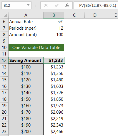
Creating Excel Data Tables

Set up a table that contains your variables going down the rows or across the columns. In this example my monthly payments are in column A.

Place your formula or a link to your formula in the cell above where your data table will place the values. In my case this is cell B12.

Next, select the cells containing the variables and the cells your results will be entered in. In this example it’s cells A12:B23. Go to the Data tab > What-if Analysis > Data Table, as shown below:

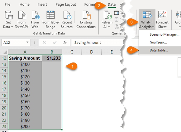
In the Data Table dialog box, shown below, select the cell that contains the variable referenced in the formula in cell B12, which is B8:

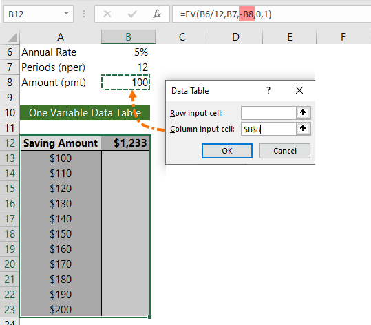
Note: As this is a single variable data table, I can leave the row input cell empty.

That’s it. Easy peasy!

Notice the formula bar in the image below contains the TABLE function. The only way the TABLE function can be entered in the worksheet is via the Data tab > What-if Analysis > Data Table. You won’t even find it in the Function Wizard.

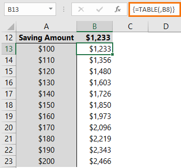
Tip: Because the data table contains a formula, you can make changes to your variables and it will automatically update.

Two Variable Data Tables

We can compare changes in the saving amount [pmt] and the interest rate [rate] using a two variable data table. In the image below I have the interest rates across row 12 and the savings amounts in column A:

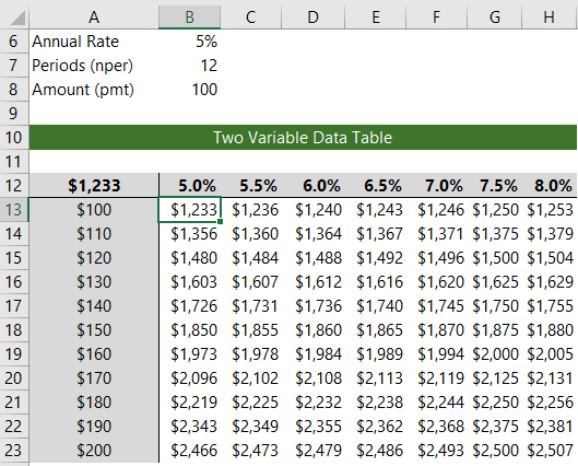
Note: your formula or a link to your formula must be in the top left cell of the table. In my case, cell A12.

The process is the same, except this time I need to select cells A12:H23 and in the Data Table dialog box I choose cell B6 as my row input cell and B8 as my column input cell:

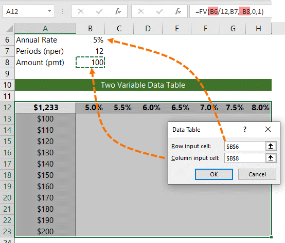
Notice the TABLE formula in the image below contains two cell references, one for the row variable and one for the column variable:

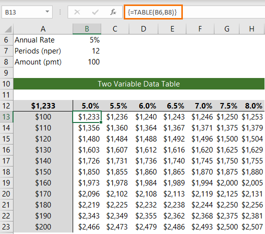
Breakeven Data Tables

There are many uses for Data Tables. Another is to calculate and visualise breakeven. With the help of Conditional Formatting heat maps we can see the breakeven curve for profit per month (in the image below) runs from 1500 pizzas at $4.00 profit per pizza through to 1200 pizzas at $5 profit per pizza:

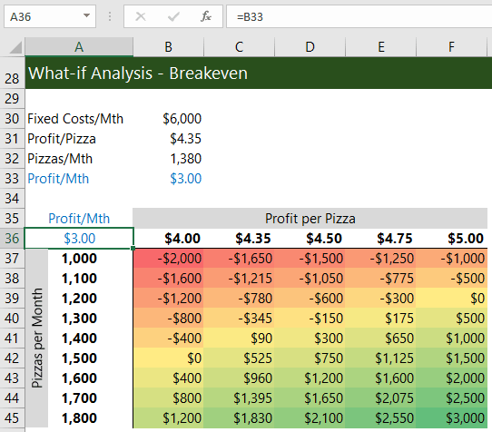
Spoiler: Of course, you could achieve the same results as a data table by inserting your formula in cells B37:F45 and simply reference the cells that contain the variables in row 36 and column A. But at least now when you stumble upon a workbook containing this mysterious TABLE function you’ll know what it is and how it got there 😉

Источник

Data Tables

One Variable Data Table

Two Variable Data Table

Calculate multiple results by using a data table

Need more help?

What is Data Table in Excel?

Table of contents

Types of Data Tables in Excel

One-Variable Data Table in Excel

Example #1

Two-Variable Data Table in Excel

Example #2

The Key Points Governing Data Tables in Excel

Frequently Asked Questions

Recommended Articles

How to Make a Data Table in Excel: Step-by-Step Guide (2023)

What is an Excel data table?

How to create a one-variable data table in Excel

Example 1: Column Input Cells

Example 2: Row Input Cells

How to create multiple one-variable data tables?

How to make a two-variable data table in Excel?

Trouble Shooting the Two-Variable Data Table

1. Editing a two-variable data table

2. Deleting a two-variable data table

That’s it – Now what?

Learn about the elements of an Excel table

Create a table

Working efficiently with your table data

Export an Excel table to a SharePoint site

Need more help?

See Also

Need more help?

One Variable Data Table

Two Variable Data Table

Data Table in Excel

How to Create Data Table in Excel?

Data Table in Excel Example #1 – One-Variable Data Table

Data Table in Excel Example #2 – Two-Variable Data Table

Things to Remember About Data Table in Excel

Recommended Articles

What are Data Tables?

How to Create Excel Data Tables

Step 1: Create a Model

Step 2: Link the Output

Step 3: Enter the Input Values

Step 4: Highlight the Cells and Access the Data Tables Function

Step 5: Link the Input Values

Step 6: Format the Data Table Output

Applications in Sensitivity Analysis

Additional Resources

How to create table from a bunch of data?

The most important thing after you create a table – Give it a name

1. Change table formatting without lifting a finger

2. Add Zebra Lines to Tables without doing Donkey Work

3. Tables come with Data Filters and Sort Options by default

4. You can also Slice your tables with slicers

5. Bye, bye cell references, welcome structured references

6. Make Calculated Columns with ease

7. Total your Tables without writing one formula

8. Convert table back to a range, if you ever need to

9. Export Tables to Pivot Tables, Woohoo

10. Push the table data to Sharepoint Intranet Site

11. Print Tables Alone, with out all the other stuff around

12. Change, reshape or clean your table data with Power Query

13. Got multiple tables? Connect them to make a multi-table pivot

So, What do you think about Excel tables?

Related Material

Get FREE Excel + Power BI Tips

Welcome to Chandoo.org

Related Tips

132 Responses to “Excel Tables Tutorial & 13 Tips for making you a Data Guru”

Leave a Reply

Watch the Video

Download the Workbook

One Variable Data Tables

Creating Excel Data Tables

Two Variable Data Tables

Breakeven Data Tables