
What is Data Table in Excel?
A Data Table in Excel helps study the different outputs obtained by changing one or two inputs of a formula. A data table does not allow changing more than two inputs of a formula. However, these two inputs can have as many possible values (to be experimented) as one wants. Excel Data tables, along with Scenarios and Goal Seek are parts of the What-If Analysis tools.
For example, an organization may want to study how changes in the cash possessed impact its working capital. A data table will help the organization know the optimum level of cash (from the specified possible values) to be held to meet its short-term obligations.
The purpose of creating data tables in Excel is to analyze the variation in outputs resulting from a change in the inputs. Moreover, one can have all the outputs in a single table which eases interpretation and allows quick sharing with other users.
Table of contents
- What is Data Table in Excel?
- Types of Data Tables in Excel
- One-Variable Data Table in Excel
- Example #1
- Two-Variable Data Table in Excel
- Example #2
- The Key Points Governing Data Tables in Excel
- Frequently Asked Questions
- Recommended Articles
- One-Variable Data Table in Excel
Types of Data Tables in Excel
The kinds of data tables in Excel are specified as follows:
- One-variable data table
- Two-variable data table
Let us discuss each type of data table one by one with the help of examples.
Note: A data table is different from a regular Excel tableIn excel, tables are a range with data in rows and columns, and they expand when new data is inserted in the range in any new row or column in the table. To use a table, click on the table and select the data range.read more. The former shows the various combinations of inputs and outputs. These outputs are calculated by considering the source dataset as the base. In contrast, an Excel table shows related data that is grouped in one place.
One-Variable Data Table in Excel
A one-variable data tableOne variable data table in excel means changing one variable with multiple options and getting the results for multiple scenarios. The data inputs in one variable data table are either in a single column or across a row.read more is created to study how a change in one input of the formula causes a change in the output. A one-variable data table in excel can be either row-oriented or column-oriented. This implies that all the possible values that an input can assume are listed in either a single row (row-oriented) or a single column (column-oriented) of Excel.
You can download this DATA Table Excel Template here – DATA Table Excel Template
Example #1
There are two images titled “image 1” and “image 2.” The following information is given:
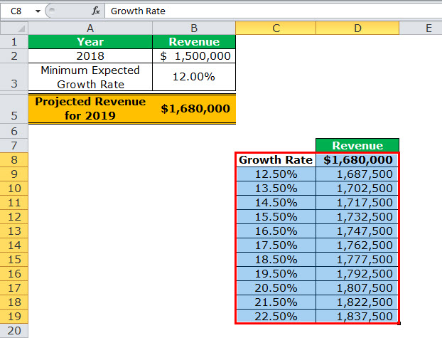
- Image 1 shows an organization’s revenue (in $) for 2018 in cell B2. The minimum growth rate expected is given as 12% in cell B3. The projected revenue (in $ in cell B5) for 2019 has been calculated by using the formula “=B2+(B2*B3).”
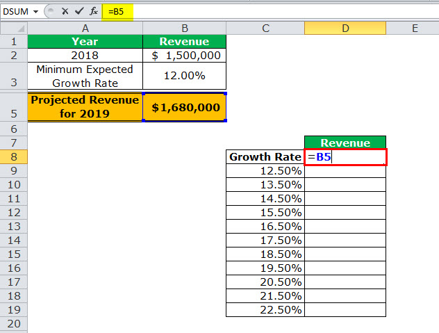
- Image 2 shows the possible values (in column C) that the growth rate can assume. The value of cell D8 has been explained in steps 1 and 2 (given further in this example).
We want to perform the following tasks:
- Calculate the projected revenues (in column D) according to the different growth rates (in column C) given in image 2.
- Create a “line with markers” chart showing the growth rates on the x-axis and the projected revenues on the y-axis. Replace the markers of the chart with arrows.
Use a one-variable data table of Excel. Interpret the data table thus created.
Image 1
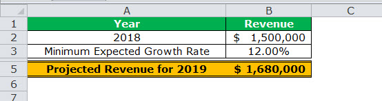
Image 2

The steps for performing the given tasks by using a one-variable data table are listed as follows:
- Enter the data of the two images in Excel. In cell D8, type “equal to” (=) followed by the reference B5. This links cell D8 to cell B5.
The linking of the two cells is shown in the following image.
Since all the growth rates have been entered vertically (C9:C19), our data table is said to be column-oriented. The entire range C8:D19 is our one-variable data table. We are creating a one-variable data table as the change in outputs will be observed against a change in one input, i.e., the growth rate.
Note: Notice that either the formula “=B2+(B2*B3)” could be typed directly in cell D8 or cell D8 can be linked to cell B5. We have chosen to link the two cells.
The linking of cell D8 to cell B5 ensures that any updates in the formula of the latter are automatically reflected in the range D9:D19 of the data table. For instance, if the formula of cell B5 is multiplied by 2 [like =B2+(B2*B3)*2], all the outputs obtained in the range D9:D19 are automatically multiplied by 2.
Had we not linked cells D8 and B5, any changes to the formula of cell B5 would not have changed the value in cell D8. Consequently, the outputs in the range D9:D19 would not have been updated automatically.

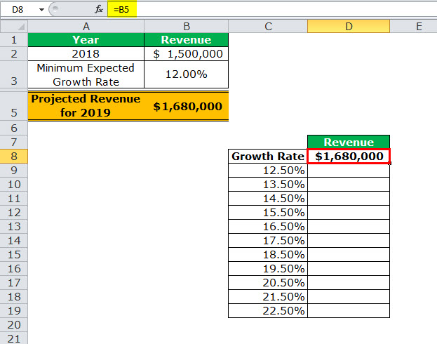
- Press the “Enter” key. Cell D8 shows the value of cell B5, as shown in the following image.
Notice that if one manually enters the value (1680000) in cell D8, the data table will not work. Moreover, one should always type the formula [=B2+(B2*B3)] or link the cell that is one row above and one column to the right of the possible input values (C9:C19). This is the reason we chose to link cell D8 to cell B5.
Note: If the data table is row-oriented, type the formula or link the cell that is one column to the left and one cell below the first possible input value. For instance, had the possible input values been in the range F2:P2, we would have entered the formula or linked cell E3 to cell B5.

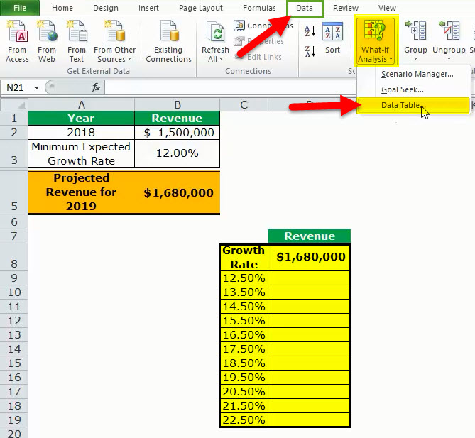
- Select the range of the data table. This selection should include the linked cell (D8), the possible input values (C9:C19), and the empty cells for outputs (D9:D19). Hence, we have selected the range C8:D19, as shown in the following image.

- From the Data tab, click the “what-if analysis” drop-down (in the “data tools” or “forecast” group). Select the option “data table.” This option is shown in the following image.

- The “data table” dialog box opens, as shown in the following image. In the box of “column input cell,” select cell B3, which contains the minimum expected growth rate. As a result, the reference $B$3 appears in this box. Leave the box of “row input cell” blank.
By giving the reference to cell B3 in the “column input cell,” we are telling Excel that at the growth rate of 12%, the projected revenue is $1,680,000. So, with this data table, Excel is being asked the projected revenue when the growth rates vary from 12.5% to 22.5%.
Note 1: A “row input cell” or “column input cell” is a reference to a cell that contains the input. This is the input that can assume the different possible values. Moreover, this input must necessarily be used in the formula whose outputs are to be studied.
In a one-variable data table, either the “row input cell” or the “column input cell” is specified depending on whether the data table is row-oriented or column-oriented.
Note 2: In a one-variable data table, Excel uses either the formula “=TABLE(row_input_cell,)” or “=TABLE(,column_input_cell)” to calculate the different outputs. The former formula is used when the possible input values are in a row, while the latter is used when the possible input values are in a column.
To view the TABLE formula, select any of the output cells and check the formula bar. In this example, the formula “=TABLE(,B3)” is used to calculate the outputs.
Further, Excel uses these TABLE formulas as array formulasArray formulas are extremely helpful and powerful formulas that are used in Excel to execute some of the most complex calculations. There are two types of array formulas: one that returns a single result and the other that returns multiple results.read more. However, these formulas cannot be edited manually, unlike the regular array formulas. But, one can delete all the output cells containing the TABLE formulas.

- Click “Ok” in the “data table” window. The range D9:D19 of the data table has been filled with values. The different outputs are shown in the following image.

Interpretation of the one-variable data table: By looking at the data table in the preceding image, one can say that when the growth rate is 12.5%, the projected revenue is $1,687,500. Likewise, when the growth rate is 13.5%, the projected revenue is $1,702,500. Hence, the larger the growth rate, the more the increase in the projected revenue.
The projected revenue is at its maximum ($1,837,500) when the growth rate is at its highest (22.5%). So, the organization can study the variation in outputs when a single input (growth rate) changes.
Note: For more examples related to the one-variable data table of Excel, refer to the hyperlink given before step 1.
- To create a “line with markers” chart that displays the growth rates on the x-axis and the projected revenues on the y-axis, follow the listed steps:
a. Select the range D9:D19 and click the Insert tab on the Excel ribbon.
b. Click the “insert line or area chart” icon from the “charts” group. Select the “line with markers” chart under the 2-D line charts. A “line with markers” chart appears, which displays the projected revenues on the y-axis.
c. Click anywhere on the chart. The “chart tools” menu becomes visible. This menu consists of the Design and Format tabs.
d. Click the Design tab of the “chart tools” menu. Choose “select data” from the “data” group. The “select data source” window opens.
e. Click “edit” under “horizontal (category) axis labels.” The “axis labels” window opens.
f. Select the range C9:C19 in the “axis label range” box. Click “Ok.” Click “Ok” again in the “select data source” window.The “line with markers” chart is created whose x-axis and y-axis look the way they are shown in the image of step 8.
- To replace the default markers of the chart with arrows, follow the listed steps:
a. Select the markers of the chart and right-click them. Choose the “format data series” option from the context menu. The “format data series” pane opens.
b. Click the “fill & line” tab. Expand the “line” tab. In “end arrow type,” select any of the arrows. We have chosen “open arrow.”
c. Select “marker” and expand the “marker options.” Choose the option “none.”
d. Close the “format data series” pane.The “line with markers” chart looks the way it is displayed in the following image. Notice that since the chart shows the projected revenues, we have titled it accordingly.


Two-Variable Data Table in Excel
A two-variable data table in excelA two-variable data table helps analyze how two different variables impact the overall data table. In simple terms, it helps determine what effect does changing the two variables have on the result.read more helps study how changes in two inputs of a formula cause a change in the output. In a two-variable data table, there are two ranges of possible values for the two inputs. From these two ranges, one range is in a row and the other is in a column of Excel.
Example #2
There are three images titled “image 1,” “image 2,” and “image 3.” The following information is given:
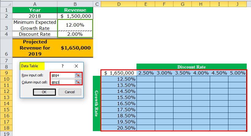
- Image 1 shows an organization’s revenue (in $ in 2018) and the minimum growth rate in cells B2 and B3 respectively. Both these figures are the same as that of the previous example. Additionally, the organization gives a 2% discount (in cell B4) to its customers. This is given to boost sales.
- Image 2 shows how the projected revenue (in $ in cell B6) for 2019 has been calculated. The formula “=B2+(B2*B3)-(B2*B4)” is used for this purpose. The amount obtained ($1,650,000) is the projected revenue after the discount.
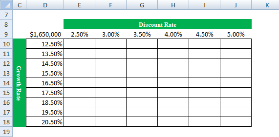
- Image 3 shows the different values in row 9 that the discount rate can assume. The possible values that the growth rate can assume are given in column D. The value of cell D9 has been explained in steps 1 and 2 (given further in this example).
Calculate the projected revenues (in E10:J18) according to the various discount rates (in row 9) and growth rates (in column D). Use a two-variable data table of Excel. Interpret the data table thus created.
Image 1

Image 2
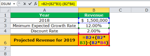
Image 3
The steps for creating a two-variable data table are listed as follows:
Step 1: Enter the data of the preceding images in Excel. In cell D9, type the “equal to” operator followed by the reference B6.
This time we have chosen to link cell D9 to cell B6. Alternatively, we could have also entered the formula [=B2+(B2*B3)-(B2*B4)] in cell D9. This is because, in a two-variable data table, one should type the formula or link the cell that is one column to the left of the first horizontal input value (2.5%). At the same time, this cell should be one row above the first vertical input value (12.5%).
The linking of cells ensures that any changes to the formula of cell B6 are reflected in the value of cell D9. Further, any change in the value of cell D9 will update the outputs (in E10:J18) automatically.
Note: Please ignore the differences in font, colors, and alignment across the images of this example. These differences may be due to the different versions of Excel being used to create the images.

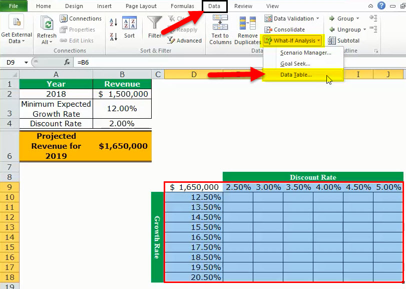
Step 2: Press the “Enter” key. Cell D9 shows the value of cell B6, which is 1,650,000. This is shown in the following image.
The entire range D9:J18 is our two-variable data table. Notice that the excel data table shows the possible discount rates horizontally (in bold in row 9) and the possible growth rates vertically (in column D). This time the variation in outputs resulting from changes in both these inputs (discount rate and growth rate) need to be studied.
Note: If the value is entered manually in cell D9, the excel data table will not work.

Step 3: Select the range D9:J18. Note that the selection should include the linked cell (D9), possible discount rates (E9:J9), possible growth rates (D10:D18), and the empty cells for the outputs (E10:J18).
The selection is shown in the following image.

Step 4: Click the “what-if analysis” drop-down (in the “data tools” or “forecast” group) of the Data tab. Select the option “data table.”
Step 5: The “data table” window opens, as shown in the following image. In the box of “row input cell,” select cell B4. In the box of “column input cell,” select cell B3. The absolute referencesAbsolute reference in excel is a type of cell reference in which the cells being referred to do not change, as they did in relative reference. By pressing f4, we can create a formula for absolute referencing.read more to cells B4 and B3 appear in the two boxes.
Cells B4 and B3 contain the minimum expected growth rate and the discount rate of the source dataset.
By making these selections, Excel is told that at a discount rate of 2% and a growth rate of 12%, the projected revenue is $1,650,000. Therefore, our two-variable data table instructs Excel to calculate the projected revenues when the discount rates and growth rates vary from 2.5% to 5% and 12.5% to 20.5% respectively.
Note: In a two-variable data table, both the “row input cell” and “column input cell” are specified, unlike a one-variable data table where one has to specify either of the two inputs.
Further a two-variable data table uses the formula “=TABLE(row_input_cell,column_input_cell)” to calculate the outputs. So, in this example, the formula “=TABLE(B4,B3)” has been used for the calculations. This formula is visible in the formula bar when an output cell is selected.
For the meaning of the “row input cell” and the “column input cell,” refer to “note 1” under step 5 of example #1.
Step 6: Click “Ok” in the “data table” window. The outputs appear in the range E10:J18, as shown in the following image.

Interpretation of the two-variable data table: When the discount rate is 2.5% and the growth rate is 12.5%, the organization’s projected revenue is $1,650,000 (in cell E10). Notice that this figure is the same as that of cell B6. However, the value in cell B6 takes into account 2% and 12% as the discount rate and growth rate respectively.
Notice that the numbers of cells E10 and B6 match those of cells G11 and I12. This implies that when the discount rate and growth rate are increased in the same proportion (like by 0.5%, 1.5% or 2.5%), the resulting value is the same as the output of the source dataset (in cell B6). Cells E10, G11, and I12 reflect 0.5%, 1.5%, and 2.5% increase in the two rates.
Likewise, had we increased both the discount and growth rates by 1%, the resulting value would have again been $1,650,000. In this case, the discount rate and growth rate would have been 3% and 13% respectively.
By obtaining the projected revenues in the range E10:J18, the organization can sell at an optimum discount rate and, at the same time, target an attainable growth rate. Hence, the organization can choose the most suitable combination of the two rates.
Note: For more examples related to the two-variable data table of Excel, click the hyperlink given before step 1 of this example.
The Key Points Governing Data Tables in Excel
The important points related to data tables of Excel are listed as follows:
- It helps select those input values that fit the business in the best possible manner.
- It facilitates the comparison of the different outputs as all the results are consolidated in one place.
- It presents the results in a tabular format that can neither be edited nor undone with the shortcut “Ctrl+Z.” The outputs can only be deleted by selecting them and pressing the “Delete” key.
- It uses the TABLE array formulas to calculate the outputs. The “row input cell” and the “column input cell” must be selected carefully to get accurate results. Moreover, the input cell or cells must be on the same worksheet as the data table.
- It need not be refreshed, unlike a pivot table. A change in the values or the formula of the source dataset causes the excel data table to update automatically.
Frequently Asked Questions
1. Define a data table and suggest when it should be used in Excel.
A data table helps analyze how a change in one or two inputs of a formula causes a change in the output. The resulting outputs are arranged in a tabular format, making them easy to compare and interpret.
A data table of Excel should be used in the following situations:
• When the outputs resulting from a change in one or two inputs need to be studied
• When the most optimum input value or values need to be chosen
• When all the combinations of inputs and outputs need to be explored in one glance
2. How to create a data table in Excel?
The steps to create a data table in Excel are listed as follows:
a. Enter the source dataset in an Excel worksheet. Use one or two inputs to calculate an output.
b. Arrange the possible values, which an input can assume, in a row and/or column.
c. Link one cell of the data table to the output cell of the source dataset. Alternatively, in a cell of the data table, enter the formula whose outputs need to be studied.
d. Select the data table. The selection should include the linked cell (or the formula cell of the data table), the possible input values, and the empty cells for outputs.
e. Select the “data table” option from the “what-if analysis” drop-down of the Data tab. The “data table” window opens.
f. Enter either the “row input cell” or “column input cell” if the impact of changing one input is to be studied. To study the impact of changing two inputs, enter both “row input cell” and “column input cell.”
g. Click “Ok” in the “data table” window.
A one-variable or two-variable data table is created depending on the execution of steps “a,” “b,” and “f.”
Note: For more details on creating a data table in Excel, refer to the examples of this article.
3. How does a data table work in Excel?
A data table works on the policy “what will be the result if one or two inputs of a formula are changed?” One cell of the data table is linked to the source dataset. In this way, Excel is told how the inputs are to be used in calculating the output.
Next, as the possible input values are supplied, Excel is asked to calculate the outputs using the same formula as that of the source dataset. The resulting table shows the different mixes of inputs and outputs, thereby assisting the user in decision-making.
Recommended Articles
This has been a guide to Data Tables in Excel. Here we discuss how to create one-variable and two-variable data tables along with practical Excel examples. You may learn more about Excel from the following articles–
- Two-Variable Data Table in ExcelA two-variable data table helps analyze how two different variables impact the overall data table. In simple terms, it helps determine what effect does changing the two variables have on the result.read more
- VBA Refresh Pivot TableWhen we insert a pivot table in the sheet, once the data changes, pivot table data does not change itself; we need to do it manually. However, in VBA, there is a statement to refresh the pivot table, expression.refreshtable, by referencing the worksheet.read more
- Merge Tables ExcelWe can use a number of different methods to merge tables in Excel, including the VLOOKUP function, the INDEX function, and the MATCH function.read more
- Data Validation in ExcelThe data validation in excel helps control the kind of input entered by a user in the worksheet.read more
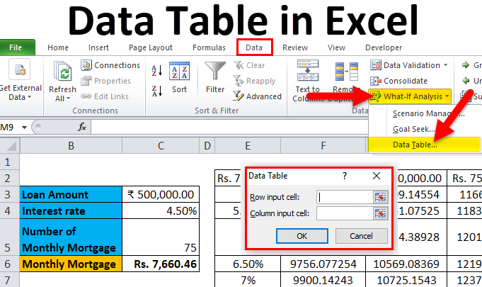
A data table is a range of cells in which you can change values in some of the cells and come up with different answers to a problem. A good example of a data table employs the PMT function with different loan amounts and interest rates to calculate the affordable amount on a home mortgage loan. Experimenting with different values to observe the corresponding variation in results is a common task in data analysis.
In Microsoft Excel, data tables are part of a suite of commands known as What-If analysis tools. When you construct and analyze data tables, you are doing what-if analysis.
What-if analysis is the process of changing the values in cells to see how those changes will affect the outcome of formulas on the worksheet. For example, you can use a data table to vary the interest rate and term length for a loan—to evaluate potential monthly payment amounts.
Types of what-if analysis
There are three types of what-if analysis tools in Excel: scenarios, data tables, and goal-seek. Scenarios and data tables use sets of input values to calculates possible results. Goal-seek is distinctly different, it uses a single result and calculates possible input values that would produce that result.
Like scenarios, data tables help you explore a set of possible outcomes. Unlike scenarios, data tables show you all the outcomes in one table on one worksheet. Using data tables makes it easy to examine a range of possibilities at a glance. Because you focus on only one or two variables, results are easy to read and share in tabular form.
A data table cannot accommodate more than two variables. If you want to analyze more than two variables, you should instead use scenarios. Although it is limited to only one or two variables (one for the row input cell and one for the column input cell), a data table can include as many different variable values as you want. A scenario can have a maximum of 32 different values, but you can create as many scenarios as you want.
Learn more in the article, Introduction to What-If Analysis.
Create either one-variable or two-variable data tables, depending on the number of variables and formulas that you need to test.
One-variable data tables
Use a one-variable data table if you want to see how different values of one variable in one or more formulas will change the results of those formulas. For example, you can use a one-variable data table to see how different interest rates affect a monthly mortgage payment by using the PMT function. You enter the variable values in one column or row, and the outcomes are displayed in an adjacent column or row.
In the following illustration, cell D2 contains the payment formula, =PMT(B3/12,B4,-B5), which refers to the input cell B3.
Two-variable data tables
Use a two-variable data table to see how different values of two variables in one formula will change the results of that formula. For example, you can use a two-variable data table to see how different combinations of interest rates and loan terms will affect a monthly mortgage payment.
In the following illustration, cell C2 contains the payment formula, =PMT(B3/12,B4,-B5), which uses two input cells, B3 and B4.
Data table calculations
Whenever a worksheet recalculates, any data tables will also recalculate—even if there has been no change to the data. To speed up calculation of a worksheet that contains a data table, you can change the Calculation options to automatically recalculate the worksheet but not the data tables. To learn more, see the section Speed up calculation in a worksheet that contains data tables.
A one-variable data table contain its input values either in a single column (column-oriented), or across a row (row-oriented). Any formula in a one-variable data table must refer to only one input cell.
Follow these steps:
-
Type the list of values that you want to substitute in the input cell—either down one column or across one row. Leave a few empty rows and columns on either side of the values.
-
Do one of the following:
-
If the data table is column-oriented (your variable values are in a column), type the formula in the cell one row above and one cell to the right of the column of values. This one-variable data table is column-oriented, and the formula is contained in cell D2.

If you want to examine the effects of various values on other formulas, enter the additional formulas in cells to the right of the first formula.
-
If the data table is row-oriented (your variable values are in a row), type the formula in the cell one column to the left of the first value and one cell below the row of values.
If you want to examine the effects of various values on other formulas, enter the additional formulas in cells below the first formula.
-
-
Select the range of cells that contains the formulas and values that you want to substitute. In the figure above, this range is C2:D5.
-
On the Data tab, click What-If Analysis > Data Table (in the Data Tools group or Forecast group of Excel 2016).
-
Do one of the following:
-
If the data table is column-oriented, enter the cell reference for the input cell in the Column input cell field. In the figure above, the input cell is B3.
-
If the data table is row-oriented, enter the cell reference for the input cell in the Row input cell field.
Note: After you create your data table, you might want to change the format of the result cells. In the figure, the result cells are formatted as currency.
-
Formulas that are used in a one-variable data table must refer to the same input cell.
Follow these steps
-
Do either of these:
-
If the data table is column-oriented, enter the new formula in a blank cell to the right of an existing formula in the top row of the data table.
-
If the data table is row-oriented, enter the new formula in a empty cell below an existing formula in the first column of the data table.
-
-
Select the range of cells that contains the data table and the new formula.
-
On the Data tab, click What-If Analysis > Data Table (in the Data Tools group or Forecast group of Excel 2016).
-
Do either of the following:
-
If the data table is column-oriented, enter the cell reference for the input cell in the Column input cell box.
-
If the data table is row-oriented, enter the cell reference for the input cell in the Row input cell box.
-
A two-variable data table uses a formula that contains two lists of input values. The formula must refer to two different input cells.
Follow these steps:
-
In a cell on the worksheet, enter the formula that refers to the two input cells.
In the following example—in which the formula starting values are entered in cells B3, B4, and B5, you type the formula =PMT(B3/12,B4,-B5) in cell C2.
-
Type one list of input values in the same column, below the formula.
In this case, type the different interest rates in cells C3, C4, and C5.
-
Enter the second list in the same row as the formula—to its right.
Type the loan terms (in months) in cells D2 and E2.
-
Select the range of cells that contains the formula (C2), both the row and column of values (C3:C5 and D2:E2), and the cells in which you want the calculated values (D3:E5).
In this case, select the range C2:E5.
-
On the Data tab, in the Data Tools group or Forecast group (in Excel 2016), click What-If Analysis > Data Table (in the Data Tools group or Forecast group of Excel 2016).
-
In the Row input cell field, enter the reference to the input cell for the input values in the row.
Type cell B4 in the Row input cell box. -
In the Column input cell field, enter the reference to the input cell for the input values in the column.
Type B3 in the Column input cell box. -
Click OK.
Example of a two-variable data table
A two-variable data table can show how different combinations of interest rates and loan terms will affect a monthly mortgage payment. In the figure here, cell C2 contains the payment formula, =PMT(B3/12,B4,-B5), which uses two input cells, B3 and B4.
When you set this calculation option, no data-table calculations occur when a recalculation is done on the entire workbook. To manually recalculate your data table, select its formulas and then press F9.
Follow these steps to improve calculation performance:
-
Click File > Options > Formulas.
-
In the Calculation options section, under Calculate, click Automatic except for data tables.
Tip: Optionally, on the Formulas tab, click the arrow on Calculation Options, then click Automatic Except Data Tables (in the Calculation group).
You can use a few other Excel tools to perform what-if analysis if you have specific goals or larger sets of variable data.
Goal Seek
If you know the result to expect from a formula, but don’t know precisely what input value the formula needs to get that result, use the Goal-Seek feature. See the article Use Goal Seek to find the result you want by adjusting an input value.
Excel Solver
You can use the Excel Solver add-in to find the optimal value for a set of input variables. Solver works with a group of cells (called decision variables, or simply variable cells) that are used in computing the formulas in the objective and constraint cells. Solver adjusts the values in the decision variable cells to satisfy the limits on constraint cells and produce the result you want for the objective cell. Learn more in this article: Define and solve a problem by using Solver.
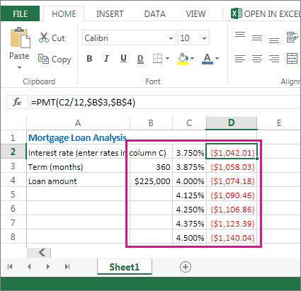
By plugging different numbers into a cell, you can quickly come up with different answers to a problem. A great example is using the PMT function with different interest rates and loan periods (in months) to figure out how much of a loan you can afford for a home or a car. You enter your numbers into a range of cells called a data table.
Here, the data table is the range of cells B2:D8. You can change the value in B4, the loan amount, and the monthly payments in column D automatically update. Using a 3.75% interest rate, D2 returns a monthly payment of $1,042.01 using this formula: =PMT(C2/12,$B$3,$B$4).
You can use one or two variables, depending on the number of variables and formulas you want to test.
Use a one-variable test to see how different values of one variable in a formula will change the results. For example, you can change the interest rate for a monthly mortgage payment by using the PMT function. You enter the variable values (the interest rates) in one column or row, and the outcomes are displayed in a nearby column or row.
In this live workbook, cell D2 contains the payment formula =PMT(C2/12,$B$3,$B$4). Cell B3 is the variable cell, where you can plug in a different term length (number of monthly payment periods). In cell D2, the PMT function plugs in the interest rate 3.75%/12, 360 months, and a $225,000 loan, and calculates a $1,042.01 monthly payment.
Use a two-variable test to see how different values of two variables in a formula will change the results. For example, you can test different combinations of interest rates and number of monthly payment periods to calculate a mortgage payment.
In this live workbook, cell C3 contains the payment formula, =PMT($B$3/12,$B$2,B4), which uses two variable cells, B2 and B3. In cell C2, the PMT function plugs in the interest rate 3.875%/12, 360 months, and a $225,000 loan, and calculates a $1,058.03 monthly payment.
Need more help?
You can always ask an expert in the Excel Tech Community or get support in the Answers community.
Data Table in Excel (Table of Contents)
- Data Table in Excel
- How to Create Data Table in Excel?
Data Table in Excel
Data tables are used to analyze the changes seen in your final result when certain variables are changed from your function or formula. Data tables are one of the existing parts of What-If analysis tools, which allow you to observe your result by experimenting it with different values of variables and to compare the outcomes stored by the data table.
There are two types of a data table, which are as follows:
- One-Variable Data Table.
- Two-Variable Data Table.
How to Create Data Table in Excel?
Data Table in Excel is very simple and easy to create. Let’s understand the working of the Data Table in Excel by Some Examples.
You can download this Data Table Excel Template here – Data Table Excel Template
Data Table in Excel Example #1 – One-Variable Data Table
One-variable data tables are efficient in the case of analyzing the changes in the result of your formula when you change the values for a single input variable.
Use case of One-Variable Data Table in Excel:
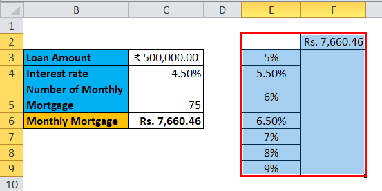
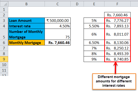
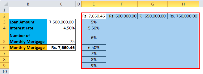
The one-variable data table is useful in scenarios where a person can observe how different interest rates change the amount of their mortgage amount to be paid. Consider the below figure, which shows the mortgage amount calculated based on the interest rate using the PMT function.
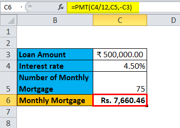
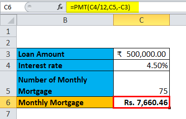
The table above shows the data where the mortgage amount is calculated based on the interest rate, mortgage period and loan amount. It uses the PMT formula to calculate the monthly mortgage amount, which can be written as =PMT (C4/12, C5,-C3).
In the case of observing the monthly mortgage amount for different interest rates, where the interest rate is considered as a variable. In order to do this, there is a need for creating a one-variable data table. The steps to create the one-variable data table are as follows:
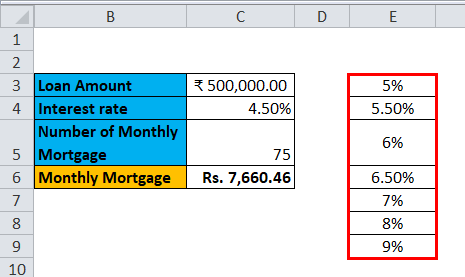
Step 1: Prepare a column which consists of different values for the interest rates. We have entered different values for interest rates in the column which is highlighted in the figure.
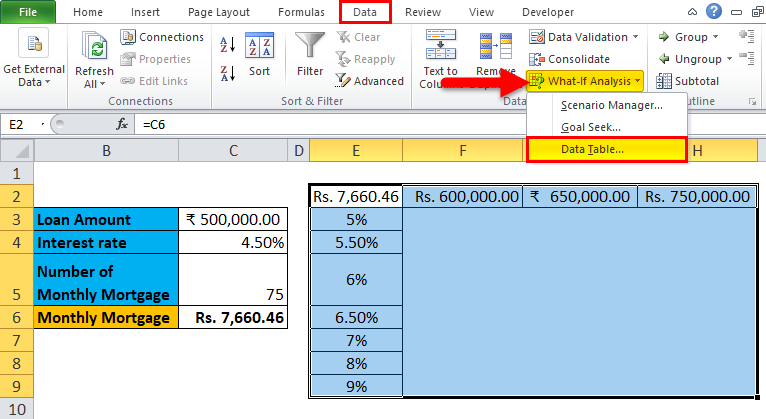
Step 2: In the cell (F2), which is one row above and diagonal to the column which you prepared in the previous step, type this = C6.
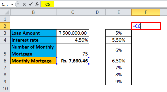
Step 3: Select the entire prepared column by values of different interest rates along with the cell where you had inserted the value, i.e. F2 cell.
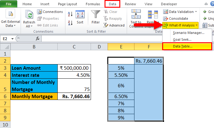
Step 4: Click on the ‘Data’ tab and select ‘What-If Analysis’, and from the options popped down, select ‘Data Table’.
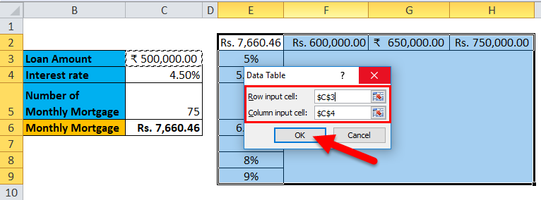
Step 5: Data table dialog box will appear.
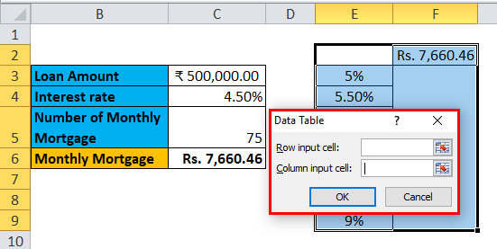
Step 6: In the Column input cell, refer to cell C4 and click OK.
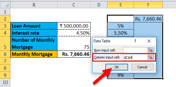
In the dialog box, we refer to the cell C4 in the Column input cell and keep the row input cell empty as we are preparing a data table with one variable.
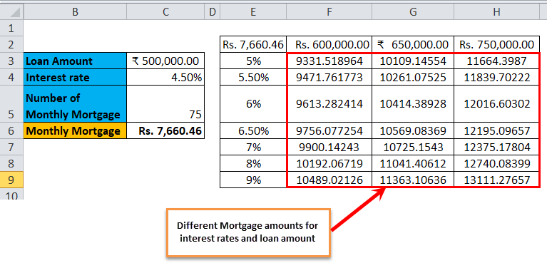
Step 7: After following all the steps, we get all the different mortgage amounts for all entered interests rates in column E (unmarked), and the different mortgage amounts are observed in column F (marked).
Data Table in Excel Example #2 – Two-Variable Data Table
Two-variable data tables are useful in scenarios where a user needs to observe the changes in the result of their formula when they change two input variables simultaneously.
Use-case of Two-Variable Data Table in Excel:
The two-variable data table is useful in scenarios where a person can observe how different interest rates and loan amounts change the amount of their mortgage amount to be paid. Instead of calculating for individual values separately, we can observe them with instantaneous results. Consider the below figure, which shows the mortgage amount calculated based on the interest rate using the PMT function.
The above example is similar to our example shown in the previous case for a one-variable data table. Here the mortgage amount in cell C6 is calculated based on the interest rate, mortgage period and loan amount. It uses the PMT formula to calculate the monthly mortgage amount, which can be written as =PMT (C4/12, C5,-C3).
In order to explain the two-variable data table with reference to the above example, we will show the different mortgage amounts and choose the best which suits you by observing the different values of interest rates and loan amount. In order to do this, there is a need for creating a two-variable data table. The steps to create the one-variable data table are as follows:
Step 1: Prepare a column which consists of different values for the interest rates and loan amount.
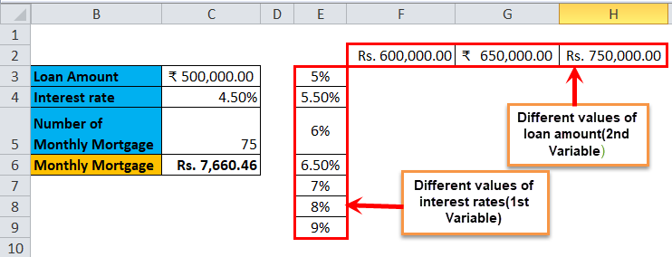
We have prepared a column consisting of the different interest rates, and in the cell diagonal to starting cell of the column, we have entered the different values of the loan amount.
Step 2: In the cell (E2), which is one row above to the column which you prepared in the previous step, type this = C6.
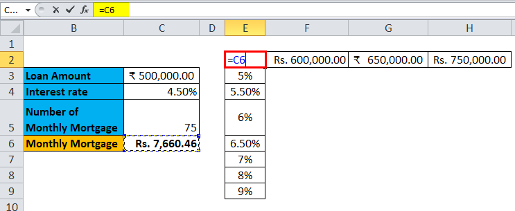
Step 3: Select the entire prepared column by values of different interest rates along with the cell where you had inserted the value, i.e. E2 cell.
Step 4: Click on the ‘Data’ tab and select ‘What-If Analysis’, and from the options popped down, select ‘Data Table’.
Step 5: A Data table dialog box will appear. The ‘Column input cell’ refers to cell C4 and in the ‘Row input cell’ C3. Both the values are selected as we are changing both the variables and Click OK.
Step 6: After following all the steps, we get different values of mortgage amounts for different values of interest rates and loan amount.
Things to Remember About Data Table in Excel
- For one variable data table, the ‘Row input cell’ is left empty, and in a two-variable data table, both ‘Row input cell’ and ‘Column input cell’ are filled.
- Once the What-If analysis is performed, and the values are calculated, you cannot change or modify any cell from the set of values.
Recommended Articles
This has been a guide to a Data Table in Excel. Here we discuss its types and how to create data table examples and downloadable excel templates. You may also look at these useful functions in excel –
- Two-Variable Data Table in Excel
- One Variable Data Table in Excel
- Excel Data Visualization
- Database Function in Excel
How to Make a Data Table in Excel: Step-by-Step Guide (2023)
Data tables in Excel are used to perform What-if Analysis on a given data set.
Using data tables, you can analyze the changes to the output value by changing the input values to a formula.
There is so much that you can do using data tables in Excel. 😀
Continue reading the article below to learn it all.
Also, download our sample workbook here to practice the examples given in this guide.
What is an Excel data table?
An Excel Data table is a What-if Analysis tool. It allows users to use different input values for a variable and assess the changes to the output value.

These are especially of help if you are operating a formula in Excel where the output depends on several variables. And you are keen to compare the results for different inputs to the formula.
Presently, Excel offers a one-variable and two-variable data table only. This means you can choose any two variable values (at max) from any formula to test.
Jump right into the article below to learn all about a data table in Excel. 🔔
How to create a one-variable data table in Excel
A one-variable data table in Excel allows users to test one variable.
For example, see the image below.

The image shows the particulars of a loan. We have three main variables in the data.
- The amount of loan
- The rate of interest/profit
- The tenure of the loan (until it is paid back)
Example 1: Column Input Cells
In this example, let’s see keep the interest rate as the variable.
What is the yearly payment to be made against the loan?
1. Write the PMT function to find the yearly repayment against the loan.
= PMT (B3, B4, B2)
= PMT (Interest Rate, Periods of Repayment, Amount of Loan Today)

2. Multiply this number by the number of payments to be made.

That’s the total amount to be paid against the loan over 5 years.
So how much is the interest on the loan?
3. Subtract the amount of loan from the amount of repayment.

Everything’s good and sorted.
Now, what if you want to see how the repayments change if one variable (the interest rate) changes?
Do not re-perform the entire calculation all over again. The Data Table (What-if analysis) will do it for you.
4. List down the variable (interest rate in this case) that is to be changed.

5. Create a link by referring to the targeted output for each interest rate in the corresponding column.
We want Excel to give us the repayments for different interest rates. So, we have created a link to the repayment in the original calculation.

6. Select the Inputs table (the interest rates and the corresponding column for targeted output).

7. Go to Data Tab > Forecast > What-If Analysis Tools > Data Table.

This will take you to the Data Table dialog box.
8. In the Column Input Cell box, create a reference to the ‘Interest Rate’ from the original table.

Reference is made to the Interest rate because that is the variable in our data. We want to experiment with how the changing interest rates affect repayments.
We have created a reference in the Column Input Cell box and not the Row Input Cell box. This is because our Input data is in the form of a column and not a row.
9. All set. Hit Okay and Ta-da! 😃

Excel creates a one-variable data table to calculate the repayments for different interest rates.
Example 2: Row Input Cells
Let’s bring a slight variation to the above data. This time the one variable of the data is the amount of the loan.
Also, let’s change the shape of Input Data from a Column to a Row.

1. Select the Inputs Data.

2. Go to Data Tab > Forecast > What-If Analysis Tools > Data Table.
3. In the ‘Data Table’ dialog box, create a reference to the Loan amount in the Row Input Cell box.

This time the variable is the amount of the loan. We want to experiment with how the changing loan amount affects the repayments.
Must note that we have created a reference to the ‘Row Input Cell’ this time. This is because our Input Data is row-oriented.
4. Click ‘Okay’ to see the repayment amount for differing amounts of loans.

What if we want to see how the total interest changes by the change in the loan amount?
Simple, refer to the amount of interest in the Inputs Data.

And there it is! Excel shows the changes to total interest instead of repayments.

How to create multiple one-variable data tables?
In the above example, what if you want to see the change in interest rates on both the repayments and total interest?
Create multiple Excel data tables. Simple.
1. In the Input Data, make two columns next to the variable interest rates.
2. In the first column, create a reference to the repayment calculation in the original data.

3. In the second column, create a reference to the total interest in the original data.

4. Create a one-variable data table by referring to the interest rate in the Column Input Cell box.

5. Click Okay, and there you go! 🙂

Excel shows the result of changes in interest rates on repayments and loan amounts.
How to make a two-variable data table in Excel?
The two-variable data table is more of a two-dimensional table. It allows you to analyze how your final output changes from the changes in any two variables of your data.
Let’s continue the example above to create a two-variable data table in Excel.
This time, let’s select two variables from the data, Interest Rate, and Loan Amount. We want to see how the repayments change when both these variables change.
1. Create a two-dimensional data table with each variable on one side of the table.

In the above image, we have set the interest rates in a columnar format. Whereas the loan amount takes the shape of a row.
2. Select the intersecting cell of both the data sides.
3. In this cell, create a reference to the calculation of the repayment in the original table.

This is because we want to see how the repayments change with changes in the interest rate and the loan amount.
Our Input Data is now ready. Let’s now create a data table and perform the What-if Analysis.
4. Select the entire Data Table.
5. Go to Data Tab > Forecast > Click What-if Analysis Tools > Data table.

6. This opens up the data table dialog box.
7. Against the Column Input Cell box, create a reference to the interest rate from the source data.

Pay attention to how a reference is created to the interest rate against the Column Input Cell. This is because the possible input values for interest rate (the first variable) are in the shape of a column.
8. Against the ‘Row Input Cell’, create a reference to the amount of loan from the source data.

The Row Input Cell refers to the amount of the loan. This is because possible input values for the loan (second variable) are in the shape of a row.
9. Click ‘Okay’, and you’re good to go.

Woah! This seems like a very densely packed data table.
What is this? See below.

Each cell of this data table is mutual to two cells. For example, in the image above, the highlighted cell shows the amount of repayment, if the interest rate changes to 12% and the loan amount changes to 2000.
Must Note: A two-variable data table is a two-dimensional table. It captures the result of the change in any two variables at the same time.
The data table formula above is an array formula. To double-check, click on any cell from the data table and see the formula bar.
You will find the formula enclosed in curly brackets. A formula enclosed in curly brackets is an Array formula.
Trouble Shooting the Two-Variable Data Table
The Two-Variable data table in Excel seems no less than magic. A heap of calculations is only a click away.
A two-variable data table is an array, and there is something you must know about a table array.
1. Editing a two-variable data table
Once you have created a two-variable data table, try clicking on any individual cell from the data table and making some changes to it.

You cannot make changes to a part of this data! This is all that Excel has to say in return.
A data table is an array, and you cannot make changes to individual cells of an array.
To make any changes to the data table, click the data table and select the whole of it.
1. From the formula bar, delete the Table formula.

2. Type in the desired value (let’s say 10) and hit Ctrl + Enter.
3. The entire table will be replaced by 10.

You can now make changes to any individual cells as it is no more an array.
2. Deleting a two-variable data table
Deleting two-variable data is a little science.
You cannot delete an individual value from the data table. However, you can only delete the whole data table.
- Select the entire array (whole data table).
- Press the delete key.
- And your data table is gone.
That’s it – Now what?
Data Tables can save you big on time.
In the article above, we have learned almost all about data tables in Excel – starting from creating a single-variable data table, and multiple single-variable data tables (in one go) to creating multiple-variable data tables.
And of course, many tips.
While data tables help data analysis in Excel, you’d need many other functions of Excel to handle big data sets in Excel. The most important of these include the VLOOKUP, SUMIF, and IF functions.
Learn each of these three functions by signing up for my free 30-minute email course that teaches you these functions (and more!).
Kasper Langmann2023-01-19T12:23:16+00:00
Page load link
Display a range of outputs in Excel given a range of different inputs
What are Data Tables?
Data tables are used in Excel to display a range of outputs given a range of different inputs. They are commonly used in financial modeling and analysis to assess a range of different possibilities for a company, given uncertainty about what will happen in the future.
How to Create Excel Data Tables
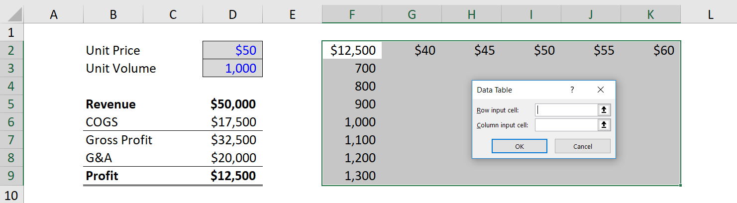
Below is a step-by-step guide on how to create an Excel data table. In the example, we will look at how much operating profit a company will generate based on different product prices and different sales volumes. We have built a simple model that assumes one variable cost (cost of goods sold), and one fixed cost (general and administrative expenses).
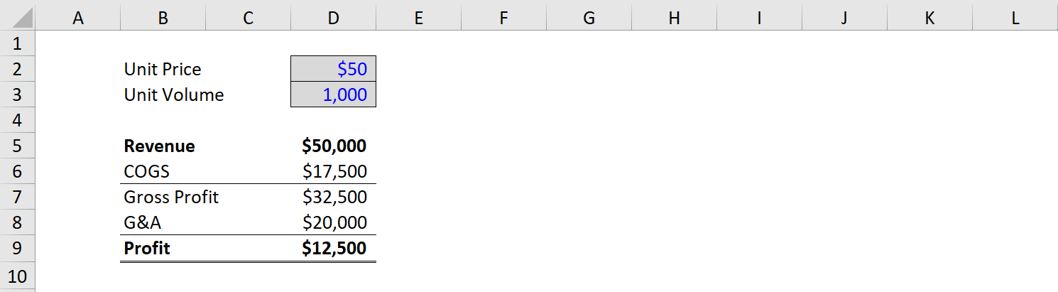
Step 1: Create a Model
The first step when creating data tables is to have a model in place. We’ve made a simple model that includes two key assumptions: unit price and unit volume. From there, we have a simple income statement that includes revenue, COGS, G&A, and operating profit (EBIT).
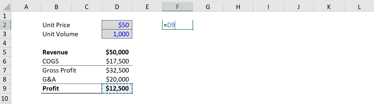
Step 2: Link the Output
Since profit is what we want to use as the output, we simply take an empty cell in the model and link it to net income at the start of the data table (the top left corner).
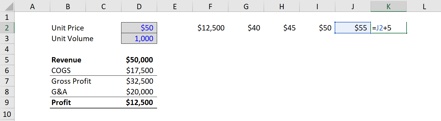
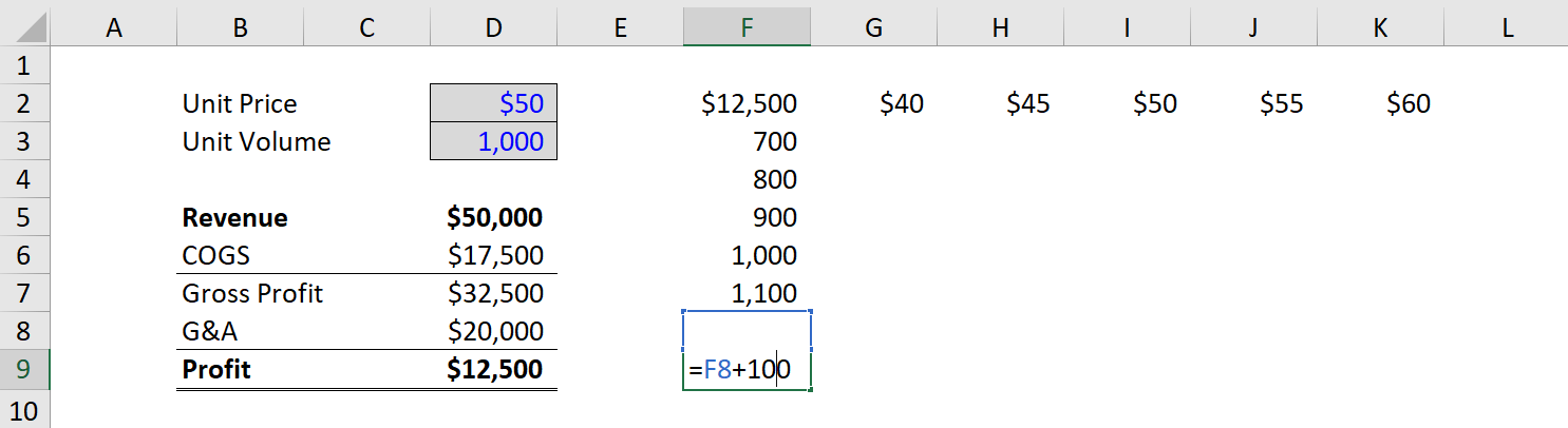
Step 3: Enter the Input Values
Once net income is linked, we need to enter the different values we want to test for unit prices and unit volumes. To do it, we manually enter the values across the top and left sides of the table. In this case, we will enter unit prices from $40 to $60 and volumes from 700 to 1,300.
To learn more about how to perform this type of analysis, check out CFI’s Sensitivity Analysis Course.
Step 4: Highlight the Cells and Access the Data Tables Function
With the structure of the table complete, the next step is to highlight all the cells with data that will be used to form the table, and then access the Excel data tables function under the Data ribbon and What-If analysis.
The keyboard shortcut on Windows is Alt, A, W, T.
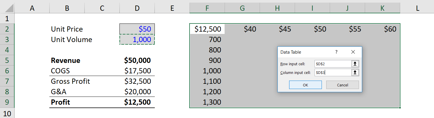
Step 5: Link the Input Values
This can be one of the trickiest steps when setting up data tables. Financial analysts often aren’t sure where the Row Input Cell goes and where the Column Input Cell goes. The easiest way to think about it that the Row refers to the assumptions across the top of the table, and the Column refers to the assumptions across the left of the table. So, link each of them to the hard-coded assumptions that drive the model.
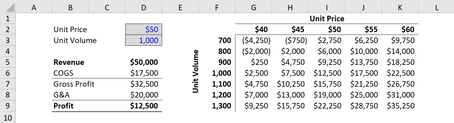
Step 6: Format the Data Table Output
Once the table is linked, it can be helpful to do some basic formatting so that the data table is easier to read. This includes adding borders and labels, so users can easily see the information contained in the analysis.
You can download the Excel file for the example we worked through together in this guide. Use it to perform your own analysis!
Download the Free Data Table template here.
Applications in Sensitivity Analysis
The main application of data tables is in performing sensitivity analysis for financial modeling and valuation. Since financial models represent a best-guess scenario on what the future holds for a business, it can be helpful to see how sensitive the value of the business is relative to various changes in assumptions.
To learn more about how to perform this type of analysis, check out CFI’s Sensitivity Analysis Course.
Additional Resources
Thank you for reading CFI’s guide to data tables, what they are, how to build them, and why they matter. To learn more and continue advancing your career, these additional CFI resources will be helpful:
- Analysis of Financial Statements
- Best Practices in Financial Modeling
- How to Link the 3 Financial Statements
- Scenario Analysis
- See all Excel resources
One Variable Data Table | Two Variable Data Table
Instead of creating different scenarios, you can create a data table to quickly try out different values for formulas. You can create a one variable data table or a two variable data table.
Assume you own a book store and have 100 books in storage. You sell a certain % for the highest price of $50 and a certain % for the lower price of $20. If you sell 60% for the highest price, cell D10 below calculates a total profit of 60 * $50 + 40 * $20 = $3800.
One Variable Data Table
To create a one variable data table, execute the following steps.
1. Select cell B12 and type =D10 (refer to the total profit cell).
2. Type the different percentages in column A.
3. Select the range A12:B17.
We are going to calculate the total profit if you sell 60% for the highest price, 70% for the highest price, etc.

4. On the Data tab, in the Forecast group, click What-If Analysis.

5. Click Data Table.

6. Click in the ‘Column input cell’ box (the percentages are in a column) and select cell C4.
We select cell C4 because the percentages refer to cell C4 (% sold for the highest price). Together with the formula in cell B12, Excel now knows that it should replace cell C4 with 60% to calculate the total profit, replace cell C4 with 70% to calculate the total profit, etc.

Note: this is a one variable data table so we leave the Row input cell blank.
7. Click OK.
Result.

Conclusion: if you sell 60% for the highest price, you obtain a total profit of $3800, if you sell 70% for the highest price, you obtain a total profit of $4100, etc.
Note: the formula bar indicates that the cells contain an array formula. Therefore, you cannot delete a single result. To delete the results, select the range B13:B17 and press Delete.
Two Variable Data Table
To create a two variable data table, execute the following steps.
1. Select cell A12 and type =D10 (refer to the total profit cell).
2. Type the different unit profits (highest price) in row 12.
3. Type the different percentages in column A.
4. Select the range A12:D17.
We are going to calculate the total profit for the different combinations of ‘unit profit (highest price)’ and ‘% sold for the highest price’.

5. On the Data tab, in the Forecast group, click What-If Analysis.
6. Click Data Table.
7. Click in the ‘Row input cell’ box (the unit profits are in a row) and select cell D7.
8. Click in the ‘Column input cell’ box (the percentages are in a column) and select cell C4.
We select cell D7 because the unit profits refer to cell D7. We select cell C4 because the percentages refer to cell C4. Together with the formula in cell A12, Excel now knows that it should replace cell D7 with $50 and cell C4 with 60% to calculate the total profit, replace cell D7 with $50 and cell C4 with 70% to calculate the total profit, etc.

9. Click OK.
Result.

Conclusion: if you sell 60% for the highest price, at a unit profit of $50, you obtain a total profit of $3800, if you sell 80% for the highest price, at a unit profit of $60, you obtain a total profit of $5200, etc.
Note: the formula bar indicates that the cells contain an array formula. Therefore, you cannot delete a single result. To delete the results, select the range B13:D17 and press Delete.
There are some Microsoft Excel features that are awesome but somewhat hidden. And the «data table analysis» is one of them.
Sometimes a formula depends on multiple inputs, and you’d like to see how different inputs values would impact the result. The data table is perfect for that situation.
This is extremely useful to analyze a problem in Excel and figure out the best solution.
The Dataset
To use the data table feature we will need some data.
Here’s a table with 2 inputs (book price and quantity sold), and a formula (revenue = price * quantity).
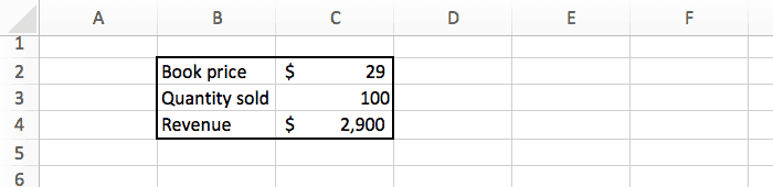
If we sell 100 books at $29 each, we will make $2,900.
The data above assume we know the book price and how many copies we will sell. But we’re actually not sure, so we’d like to know the revenue for different combination of price and quantity. For example: how much profit will we make if we sell 150 copies instead of 100, and what if the price is $19 or $49?
There are 2 main ways to do that:
- Manually change the 2 inputs, and see how the result change.
- Do that automatically with the data table feature.
Nobody likes doing repetitive tasks manually, so let’s try the second option 
The Set Up
Before we start using the data table, we need to do some changes to our data.
First we need to copy the formula to a separate place. You can do this by simply typing =C4 in a blank cell.
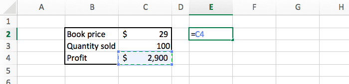
Then we need to tell Excel what values we would like to test. To the right of the formula we list all the prices ($19, $29, $49), and below the formula we list all the quantities (25, 50, 100).
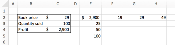
And we can add some basic formatting (borders and currency) to make things look slightly better.
Our goal is to fill this table with the profit for each combination of price and quantity.
Data Table Example
Now we can start the interesting part!
Select the new table we just created, and in the «data» tab, click on the «what if analysis» button. There select «data table».
A popup will appear that you need to fill like this:
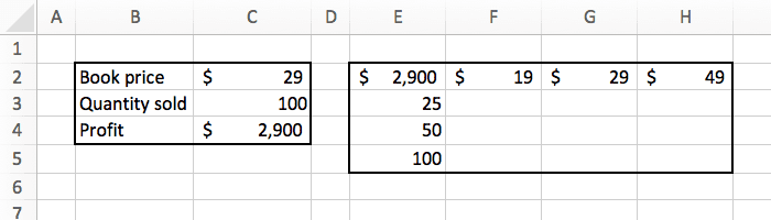
- Row input cell: we listed the price at the top, so the «row input» is the price, which is in C2.
- Column input cell»: we listed the quantity in the left, so the «column input» is the quantity, which is in C3.
Press OK, and we are done. Excel did the math for us, and automatically updated the spreadsheet with all the numbers we wanted.
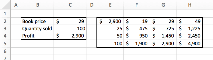
Now we can see exactly how much revenue we will make based on the different combination of inputs. For example it shows that selling 50 copies at $49 will make us $2,450. That’s super powerful.
Limitations
For your information, using data tables have some drawbacks. Here I listed three limitations that make me most uncomfortable:
- The performance and calculation speed of an Excel file will be slowed down if it contains many data tables.
- The structure of the data table is fixed. You will get an error message if you try to insert a row or column in a data table, or if you delete just a single cell in it.
- The data table must be located on the same tab as the setup data table (as mentionned above in the Set Up section). You cannot link the data table to cells on a different tab.
Conclusion
With just a few clicks, we can get Excel to do some magic computation and give us interesting information.
For this example we had a simple formula. But you could do the same on something much more complex, and Excel will give you the perfect answer in no time.
Excel Data Tables are one of the What-if Analysis tools that we have available to aid our decision making. They don’t require knowledge of any new fancy formulas and are super quick to build.
With Excel Data Tables we can perform what-if analysis with one or two variables, which makes it quick and easy to experiment and understand the outcome of different options.
Watch the Video

Download the Workbook
Enter your email address below to download the sample workbook.
By submitting your email address you agree that we can email you our Excel newsletter.
One Variable Data Tables
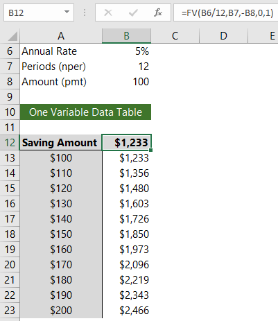
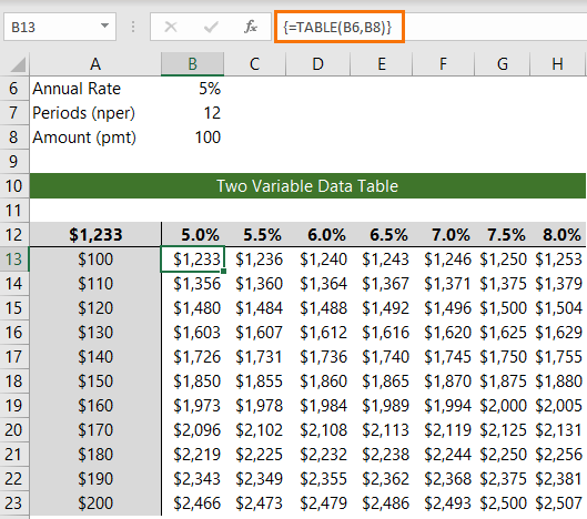
In cell B12 (image below) I’ve used the FV function (future value) to calculate the amount we’ll have after 12 months of saving $100 at the beginning of each month at a 5% interest rate p.a., which results in $1233.
Note: The FV function syntax is:
=FV(rate, nper, [pmt], [pv], [type])
I’ll be adjusting the pmt argument in this one variable data table what-if analysis.
What if we increased our monthly savings amount by $10 or $20 or more? It’s easy to see the effect of the change in the savings amount [pmt] with a Data Table:
Creating Excel Data Tables
Set up a table that contains your variables going down the rows or across the columns. In this example my monthly payments are in column A.
Place your formula or a link to your formula in the cell above where your data table will place the values. In my case this is cell B12.
Next, select the cells containing the variables and the cells your results will be entered in. In this example it’s cells A12:B23. Go to the Data tab > What-if Analysis > Data Table, as shown below:
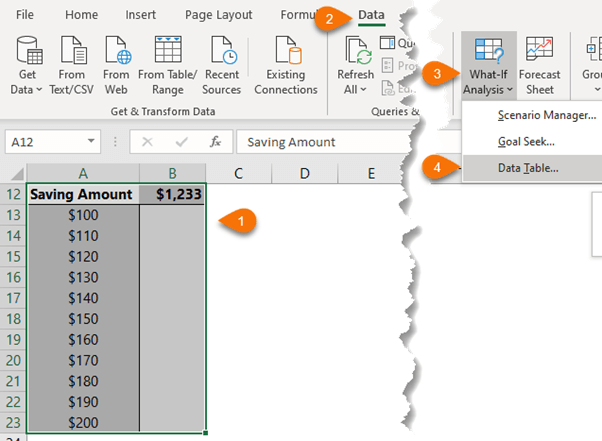
In the Data Table dialog box, shown below, select the cell that contains the variable referenced in the formula in cell B12, which is B8:
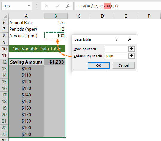
Note: As this is a single variable data table, I can leave the row input cell empty.
That’s it. Easy peasy!
Notice the formula bar in the image below contains the TABLE function. The only way the TABLE function can be entered in the worksheet is via the Data tab > What-if Analysis > Data Table. You won’t even find it in the Function Wizard.
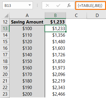
Tip: Because the data table contains a formula, you can make changes to your variables and it will automatically update.
Two Variable Data Tables
We can compare changes in the saving amount [pmt] and the interest rate [rate] using a two variable data table. In the image below I have the interest rates across row 12 and the savings amounts in column A:
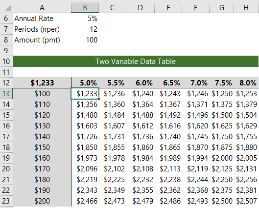
Note: your formula or a link to your formula must be in the top left cell of the table. In my case, cell A12.
The process is the same, except this time I need to select cells A12:H23 and in the Data Table dialog box I choose cell B6 as my row input cell and B8 as my column input cell:
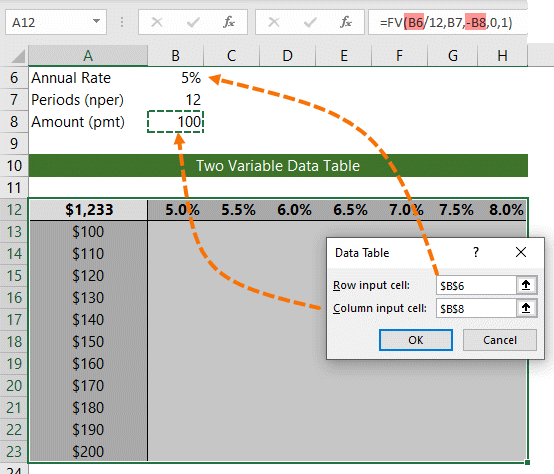
Notice the TABLE formula in the image below contains two cell references, one for the row variable and one for the column variable:
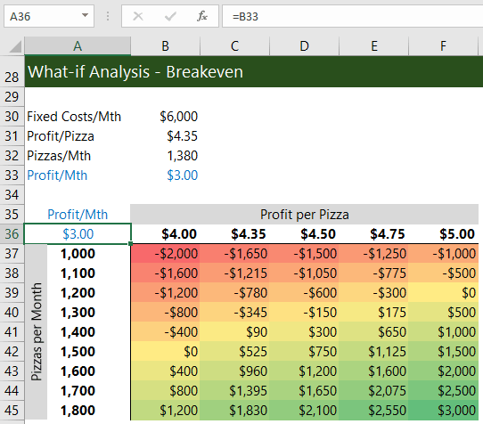
Breakeven Data Tables
There are many uses for Data Tables. Another is to calculate and visualise breakeven. With the help of Conditional Formatting heat maps we can see the breakeven curve for profit per month (in the image below) runs from 1500 pizzas at $4.00 profit per pizza through to 1200 pizzas at $5 profit per pizza:
Spoiler: Of course, you could achieve the same results as a data table by inserting your formula in cells B37:F45 and simply reference the cells that contain the variables in row 36 and column A. But at least now when you stumble upon a workbook containing this mysterious TABLE function you’ll know what it is and how it got there 😉
In this post, we’re going to learn everything there is to know about Excel Tables!
Yes, I mean everything and there’s a lot.
This post will tell you about all the awesome features Excel Tables have and why you should start using them.
What is an Excel Table?
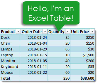
Excel Tables are containers for your data.
Imagine a house without any closets or cupboards to store your things, it would be chaos! Excel tables are like closets and cupboards for your data, they help to contain and organize data in your spreadsheets.
In your house, you might put all your plates into one kitchen cupboard. Similarly, you might put all your customer data into one Excel table.
Tables tell excel that all the data is related. Without a table, the only thing relating the data is proximity to each other.
Ok, so what’s so great about Excel Tables other than being a container to organize data? A lot actually. This post will tell you about all the awesome features tables have and should convince you to start using them.
Video Tutorial
The Parts of a Table
Throughout this post, I’ll be referring to various parts of a table, so it’s probably a good idea that we’re both talking about the same thing.
This is the Column Header Row. It is the first row in a table and contains the column headings that identify each column of data. Column headings must be unique in the table, they cannot be blank and they cannot contain formulas.
This is the Body of the table. The body is where all the data and formulas live.
This is a Row in the table. The body of a table can contain one or more rows and if you try to delete all the rows in a table a single blank row will remain.
This is a Column in the table. A table must contain at least one column.
This is the Total Row of the table. By default, tables don’t include a total row but this feature can be enabled if desired. If it’s enabled, it will be the last row of the table. This row can contain text, formula or remain blank. Each cell in the total row will have a drop down menu that allows selection of various summary formula.
Create a Table from the Ribbon
Creating an Excel Table is really easy. Select any cell inside your data and Excel will guess the range of your data when creating the table. You’ll be able to confirm this range later on. Instead of letting Excel guess the range you can also select the entire range of data in this step.
With the active cell inside your data range, go to the Insert tab in the ribbon and press the Table button found in the Tables section.
The Create Table dialog box will pop up. Excel guesses the range and you can adjust this range if needed using the range selector icon on the right hand side of the Where is the data for your table? input field. You can also adjust this range by manually typing over the range in the input field.
Checking the My table has headers box will tell Excel the first row of data contains the column headers in your table. If this is unchecked Excel will create generic column headers for the table labelled Column 1, Column 2 etc…
Press the Ok button when you’re satisfied with the data range and table headers check box.
Congratulations! You now have an Excel table and your data should look something like the above depending on the default style of your tables.
Contextual Table Tools Design Tab
Whenever you select a cell inside a table, you will notice a new tab appear in the ribbon labelled Table Tools Design. This is a contextual tab and only appears when a table is selected. When the active cell moves outside the table, the tab will disappear again.
This is where all the commands and options related to tables will live. This is where you’ll be able to name your table, find table related tools, enable or disable table elements and change your table’s style.
Create a Table with a Keyboard Shortcut
You can also create a table using a keyboard shortcut. The process is the same as described above but instead of using the Table button in the ribbon you can press Ctrl + T on your keyboard. It’s easy to remember since T is for Table!
There is actually another keyboard shortcut that you can use to create tables, Ctrl + L will also do the same thing. This is a legacy from when tables were called lists (L is for List).
Name a Table
Anytime you create a new table Excel will give it an initial generic name starting with Table1 and increasing sequentially. You should always rename your table with a descriptive and short name.
Not all names are allowed. There are a few rules for a table name.
- Each table must have a unique name within a workbook.
- You can only use letters, numbers and the underscore character in a table name. No spaces or other special characters are allowed.
- A table name must begin with either a letter or an underscore, it can not begin with a number.
- A table name can have a maximum of 255 characters.
Select any cell inside your table and the contextual Table Tools Design tab will appear in the ribbon. Inside this tab you can find the Table Name under the Properties section. Type over the generic name with your new name and press the Enter button when finished to confirm the new name.
Rename a Table
Renaming a table you’ve already named is the same process as naming a table for the first time. If you think about it, when you first name a table you’re actually renaming it from the generic name of Table1 to a new name.
So go back to the Table Tools Design tab and type your new name over the old one in the Table Name and press Enter. Easy, and the name is changed.
Changing your table name this way requires navigating to your table and selecting a cell within it, so it can be tedious if you need to rename a lot of tables across different sheets in your workbook. Instead, you can change any of your table names without going to each table using the Name Manager.
Go to the Formula tab and press the Name Manager button in the Defined Names section. You’ll be able to see all your named objects here. The table objects will have a small table icon to the left of the name. You can filter to show only the table objects using the Filter button in the upper right hand corner and selecting Table Names from the options.
You can then edit any name by selecting the item and pressing the Edit button. You’ll be able to change the name and add some comments to describe the data in your table.
Navigate Tables with the Name Box
You can easily navigate to any table in your workbook using the name box the the left of the formula bar. Click on the small arrow on the right side of the name box and you will see all table names in the workbook listed. Click on any of the tables listed and you will be taken to that table.
Convert a Table Back to a Normal Range
Ok, you changed your mind and don’t want your data inside a table anymore. How do you convert it back into a regular range?
If changing it to a table was the last thing you did, Ctrl + Z to undo your last action is probably the quickest way.
If it wasn’t the last thing you did, then you’re going to need to use the Convert to Range command found in the Table Tools Design tab under the Tools section.
You’ll be prompted to confirm that you really want to convert the table to a normal range. Noooooo, don’t do it, tables are awesome!
If you click on yes, then all the awesome benefits from tables will be gone except for the formatting design. You’ll need to manually clear this from the range if you want to get rid it. You can do this by going to the Home tab then pressing the Clear button found in the Editing section, then selecting Clear Formats.
This can also be done from the right click menu. Right click anywhere in the table and select Table from the menu and then Convert to Range.
Select the Entire Column
If your data is not inside a table then selecting an entire column of the data can be difficult. The usual way would be to select the first cell in the column and then hold Ctrl + Shift then press the Down arrow key. If the column has blank cells, then you might need to press the Down arrow key a few times until you reach the end of the data.
The other option is to select the first cell and then use the scroll bar to scroll to the end of your data then hold the Shift key while you select the last column.
Both options can be tedious if you have a lot of data or there are a lot of blanks cells in the data.
With a table, you can easily select the entire column regardless of blank cells. Hover the mouse cursor over the column heading until it turns into a small arrow pointing down then left click and the entire column will be selected. Left click a second time to include the column heading and any total row in the selection.
Another way to quickly select the entire column is to place the active cell cursor on any cell in the column and press Ctrl + Space. This will select the entire column excluding the column header and total row. Press Ctrl + Space again to include the column headers and total row.
Select the Entire Row
Selecting the entire row is just as easy. Hover the mouse cursor over the left side of the row until it turns into a small arrow pointing left then left click and the entire row will be selected. This works on both the column heading row and total row.
Another way to quickly select the entire row is to place the active cell cursor on any cell in the row and press Shift + Space.
Select the Entire Table
It’s also possible to select the entire table and there are a couple different ways to do this.
You can place the active cell cursor inside the table and press Ctrl + A. This will select the entire body of the table excluding the column headers and total row. Press Ctrl + A again to include the column headers and total row.
Hover the mouse over the top left hand corner of the table until the cursor turns into a small black diagonal right and downward pointing arrow. Left click once to select only the body. Left click a second time to include the header row and total row.
You can also select the table with the mouse. Place the active cell inside the table and then hover the mouse cursor over any edge of the table until it turns into a four way directional arrow then left click. This will also select the column headers and total row.
Select Parts of the Table from the Right Click Menu
You can also select rows, columns or the entire table using the right click menu. Right click anywhere on the row or column you want to select then choose Select and pick from the three options available.
Add a Total Row
You can add a total row which allows you to display summary calculations in the last row of your table.
Adding summary calculations at the bottom of your data can be dangerous as they might end up getting included by accident in a pivot table using the data. This is another advantage of tables, as the total row won’t be included in any pivot tables created with the table.
To enable the total row, go to the Table Tools Design tab and check the Total Row box found in the Table Style Options section.
You can temporarily disable the total row without losing the formulas you added to it. Excel will remember the formulas you had and they will appear when you enable it again.
Each cell in the total row has a drop down menu that allows you to pick various aggregating functions to summarize the column of data above.
You can also enter your own formulas. I’ve entered a SUMPRODUCT formula in the Unit Price total to sum the Quantity x Unit Price to calculate a total sale amount. Formulas don’t have to return a number, they can also be text results.
Constant numerical or text values are also allowed anywhere in the total row. In fact the leftmost column will usually contain the text Total by default.
Add a Total Row with a Right Click
You can also add the total row with a right click. Right click anywhere on the table and the choose Table and Total Row from the menu.
Add a Total Row with a Keyboard Shortcut
Another way to quickly add the total row is to place the active cell cursor inside your table and use the Ctrl + Shift + T keyboard shortcut.
Disable the Column Header Row
The column header row is enabled by default, but you can disable it. This doesn’t delete the column headers, it’s essentially like hiding them as you will still reference columns based on the column header name.
Go to the Table Tools Design tab and uncheck the Total Row box found in the Table Style Options section.
Add Bold Format to the First or Last Columns
You can enable a bold formatting on either your first or last column to highlight it and draw attention to them over other columns.
Go to the Table Tools Design tab and check either of the First Column or Last Column boxes (or both) found in the Table Style Options section.
Add Banded Rows or Columns
Banded rows are already enabled by default, but you can turn them off if you want. Banded columns are disabled by default, so you need to enable them if you want them.
To enable or disable either, go to the Table Tools Design tab and check or uncheck the Banded Rows or Banded Columns boxes found in the Table Style Options section.
I generally find banded rows are the most useful and if you enable banded columns at the same time, the table starts to look a little messy. I recommend one or the other and not both at the same time.
- Table with no banded rows or columns.
- Table with banded rows only.
- Table with banded columns only.
- Table with both banded rows and columns.
Table Filters
By default, the table filters option is enabled. You can disable them from the Table Tools Design tab by unchecking the Filter Button box found in the Table Style Options section.
You can also toggle the filters on or off from the active table by using the regular filter keyboard shortcut of Ctrl + Shift + L.
If you left click on any of the filters, it will bring up the familiar filter menu where you can sort your table and apply various filters depending on the type of data in the column.
The great thing about table filters is you can have them on multiple tables in the same sheet simultaneously. You will need to be careful though as filtered items in one table will affect the other tables if they share common rows. You can only have one set of filters at a time in a sheet of data without tables.
Total Row with Filters Applied
When you select a summary function from the drop down menu in the total row, Excel will create the corresponding SUBTOTAL formula. This SUBTOTAL formula ignores hidden and filtered items. So when you filter your table these summaries will update accordingly to exclude the filtered values.
Note that the SUMPRODUCT formula in the Unit Price column still includes all the filtered values while the SUBTOTAL sum formula in the Quantity column does not.
Column Headers Remain Visible When Scrolling
If you scroll down while the active cell is in a table, its column headers will remain visible along with the filter buttons. The table’s column headings will get promoted into the sheet’s column headings where we would normally see the alphabetic column name.
This is extremely handy when dealing with long tables as you won’t need to scroll back up to the top to see the column name or use the filters.
Automatically Include New Rows and Columns
If you type or copy and paste new data into the cells directly below a table, they will automatically be absorbed into the table.
The same thing happens when you type or copy and paste into the cells directly to the right of a table.
Automatically Fill Formulas Down the Entire Column
When you enter a formula inside a table it will automatically fill the formula down the entire column.
Even when a formula has already been entered and you add new data to the row directly below the table any existing formulas will automatically fill.
Editing an existing formula in any of the cells will also update the formula in the entire column. You’ll never forget to copy and paste down a formula again!
Turn Off the Auto Include and Auto Fill Settings
You can turn off the feature that automatically adds new rows or columns and fills down formulas.
Go to the File tab and select Options. Choose Proofing then press the AutoCorrect Options button. Navigate to the AutoFormat As You Type tab in the AutoCorrect dialog box.
Unchecking the Include new rows and columns in table option allows you to type directly underneath or to the right of a table without it absorbing the cells.
Unchecking the Fill formulas in tables to create calculated columns option means the formulas in a table will no longer automatically fill down the column.
Resize with the Handle
Every table comes with a Size Handle found in the bottom rightmost cell of the table.
When you hover the mouse over the handle, the cursor will turn into a double-sided diagonally slanting arrow and you can then click and drag to resize the table. You can either expand or contract the size. Data will be absorbed into the table or removed from it accordingly.
Resize with the Ribbon
You can also resize the table from the ribbon. Go to the Table Tools Design tab and press the Resize Table command in the Properties section.
The Resize Table dialog box will pop up and you’ll be able to select a new range for your table. Use the range selector icon to select a new range. You can select either a larger or smaller range, but The table headers will need to remain in the same row and the new table range must overlap the old table range.
Add a New Row with the Tab Key
You can add a new blank row to a table with the Tab key. Place the active cell cursor inside the table on the cell containing the sizing handle and press the Tab key.
The tab key act like a carriage return and the active cell is taken to the rightmost cell on a new line that’s added directly below.
This is a handy shortcut to know because when the total row is enabled, it’s not possible to add a new row by typing or copying and pasting data directly below the table.
Insert Rows or Columns
You can insert extra rows or columns into a table with a right click. Select a range in the table and right click then choose Insert from the menu. You can then either choose to insert Table Columns to the Left or Table Rows Above.
Table Columns to the Left will insert the number of columns selected to the left of the selection and the number of rows in the selection is ignored.
Table Rows Above will insert the number of rows selected just above the selection and the number of columns in the selection is ignored.
Delete Rows or Columns
Deleting rows or columns has a similar story to inserting them. Select a range in the table and right click then choose Delete from the menu. You can then either choose to delete Table Columns or Table Rows.
Formats in a Table Automatically Apply to New Rows
When you add new data to your table, you don’t need to worry about applying formatting to match the rest of the data above. Formatting will automatically fill down from above if the formatting has been applied to the entire column.
I’m not just talking about the table style formats. Other formatting like dates, numbers, fonts, alignments, borders, conditional formatting, cell colours etc. will all automatically fill down if they’ve been applied to the whole column.
If you’ve formatted all your numbers as a currency in a column and you add new data, it too will get the currency format applied to it.
You never need to worry about inconsistent formatting in your data.
Add a Slicer
You can add a slicer (or several) to a table for an easy to use filter and visual way to see what items the table is filtered on.
Go to the Table Tools Design tab and press the Insert Slicer button found in the Tools section.
Change the Style
Changing the styling of a table is quick and easy. Go to the Table Tools Design select a new style from the selection found in the Table Styles section. If you left click the small downward arrow on the right hand side of the styles palette, it will expand to show all available options.
These table styles apply to the whole table and will also apply to any new rows or columns added later on.
There are many options to choose from including light, medium and dark themes. As you hover over the various selections, you’ll be able to see a live preview in the worksheet. The style won’t actually change until you click on one though.
You can even create your own New Table Style.
Set a Default Table Style
You can set any of the styles available as the default so that when you create a new table you don’t need to change the style. Right click on the style you want to set as the default and then choose Set As Default from the menu.
Unfortunately, this is a workbook level setting and will only affect the current workbook. You will need to set the default for each workbook you create if you don’t want the application default option.
Only Print the Selected Table
When you place the active cell cursor inside a table and then try to print, there is an option to only print the selected table. Go to the Print menu screen by either going to the File tab and selecting Print or using the Ctrl + P keyboard shortcut, then select Print Selected Table in the settings.
This will remove any items from the print area that are not in the table.
Structured Referencing
Tables come with a useful feature called structured referencing which helps to make range references more readable. Ranges within a table can be referred to using a combination of the table name and column headings.
Instead of seeing a formula like this =SUM(D3:D9) you might see something like this =SUM(Sales[Quantity]) which is much easier to understand the meaning of.
This is why naming your table with a short descriptive name and column headings is important as it will improve the readability of the structured references!
When you reference specific parts of a table, Excel will create the reference for you so you don’t need to memorize the reference structure but it will help to understand it a bit.
Structured references can contain up to three parts.
- This is the table name. When referencing a range from inside the table this part of the reference is not required.
- These are range identifiers and identify certain parts of the reference for a table like the headers or total row.
- These are the column names and will either be a single column or a range of columns separated by a full colon.
Example of structured References for a Row
=Sales[@[Unit Price]]will reference a single cell in the body.=Sales[@[Product]:[Unit Price]]will reference part of the row from the Product column to the Unit Price column including all columns in between.=Sales[@]will reference the full row.
Example of Structured References for Columns
=Sales[Unit Price]will reference a single column and only include the body.=Sales[[#Headers],[#Data],[Unit Price]]will reference a single column and include the column header and body.=Sales[[#Data],[#Totals],[Unit Price]]will reference a single column and include the body and total row.=Sales[[#All],[Unit Price]]will reference a single column and include the column header, body and total row.
Example of Structured References for the Total Row
=Sales[#Totals]will reference the entire total row.=Sales[[#Totals],[Unit Price]]will reference a cell in the total row.=Sales[[#Totals],[Product]:[Unit Price]]will reference part of the total row from the Product column to the Unit Price column including all columns in between.
Example of Structured References for the Column Header Row
=Sales[#Headers]will reference the entire column header row.=Sales[[#Headers],[Order Date]]will reference a cell in the column header row.=Sales[[#Headers],[Product]:[Unit Price]]will reference part of the column header row from the Product column to the Unit Price column including all columns in between.
Example of Structured References for the Table Body
=Saleswill reference the entire body.=Sales[[#Headers],[#Data]]will reference the entire column header row and body.=Sales[[#Data],[#Totals]]will reference the entire body and total row.=Sales[#All]will reference the entire column header row, body and total row.
Using Intellisense
One of the great things about a table is the structured references will appear in Intellisense menus when writing formulas. This means you can easily write a formula using the structured references without remembering all the fields in your table.
After typing the first letter of the table name, the IntelliSense menu will show the table name among all the other objects starting with that letter. You can use the arrow keys to navigate to it and then press the Tab key to autocomplete the table name in your formula.
If you want to reference a part of the table, you can then type a [ to bring up all the available items in the table. Again, you can navigate with the arrow keys and then use the Tab key to autocomplete the field name. Then you can close the item with a ].
Turn Off Structured Referencing
If you’re not a fan of being forced to use the structured referencing system, then you can turn it off. Any formulas that have been entered using the structured referencing will remain and they will still work the same. You’ll also still be able to use structured references, Excel just won’t automatically create them for you.
To turn it off, go to the File tab and then select Options. Choose Formulas on the side pane and then uncheck the Use table names in formulas box and press the Ok button.
Summarize with a PivotTable
You can create a pivot table from your table in Table Tools Design tab, press the Summarize with PivotTable button found in the Tools section. This will bring up the Create PivotTable window and you can create a pivot table as usual.
This is the same as creating a pivot table from the Insert tab and doesn’t give any extra options specific to tables.
Remove Duplicates from a Table
You can create remove duplicate rows of data from your table in Table Tools Design tab, press the Remove Duplicates button found in the Tools section. This will bring up the Remove Duplicates window and delete duplicate values for one or more columns in the table.
This is the same as removing duplicates from the Data tab and doesn’t give any extra options specific to tables.
About the Author
John is a Microsoft MVP and qualified actuary with over 15 years of experience. He has worked in a variety of industries, including insurance, ad tech, and most recently Power Platform consulting. He is a keen problem solver and has a passion for using technology to make businesses more efficient.