
Excel for Microsoft 365 Excel 2021 Excel 2019 Excel 2016 Excel 2013 Excel 2010 Excel 2007 More…Less
You can use Excel to create and edit connections to external data sources that are stored in a workbook or in a connection file. You can easily manage these connections, including creating, editing, and deleting them using the current Queries & Connections pane or the Workbook Connections dialog box (available in previous versions).
Data in an Excel workbook can come from two different locations. The data may be stored directly in the workbook, or it may be stored in an external data source, such as a text file, a database, or an Online Analytical Processing (OLAP) cube. The external data source is connected to the workbook through a data connection, which is a set of information that describes how to locate, log in, query, and access the external data source.
When you are connected to an external data source, you can also perform a refresh operation to retrieve the updated data. Each time that you refresh data, you see the most recent version of the data, including any changes that were made to the data since it was last refreshed.
Connection information can either be stored in the workbook or in a connection file, such as an Office Data Connection (ODC) file (.odc) or a Universal Data Connection (UDC) file (.udcx). Connection files are particularly useful for sharing connections on a consistent basis and for facilitating data source administration.
If you use a connection file to connect to a data source, Excel copies the connection information from the connection file into the Excel workbook. When you make changes by using the Connection Properties dialog box, you are editing the data connection information that is stored in the current Excel workbook, and not the original data connection file that may have been used to create the connection, indicated by the file name that is displayed in the Connection File property. Once you edit the connection information (with the exception of the Connection Name and Connection Description properties), the link to the connection file is removed and the Connection File property is cleared.
By using the Connection Properties dialog box or the Data Connection Wizard, you can use Excel to create an Office Data Connection (ODC) file (.odc). For more information, see Connection properties and Share data with ODC.
-
Do one of the following:
-
Create a new connection to the data source. For more information, see Move data from Excel to Access, Import or export text files, or Connect to SQL Server Analysis Services Database (Import).
-
Use an existing connection. For more information, see Connect to (Import) external data.
-
-
Save the connection information to a connection file by clicking Export Connection File on the Definition tab of the Connection Properties dialog box to display the File Save dialog box, and then save the current connection information to an ODC file.
Note The Queries & Connections pane is available in Microsoft Office 365 for Excel and Excel stand-alone version 2019 or later. It replaced the Workbook Connections dialog box which is available in Excel stand-alone versions 2010, 2013, and 2016.
The Queries & Connections pane (Select Data > Queries & Connections) In one location, you can get to all the information and commands you need to work with your external data. This pane has two tabs:
-
Queries Displays all the queries in the workbook. Right click a query to see available commands. For more information, see Manage queries.
-
Connections
Displays all the connections in the workbook. Right click a connection to see available commands. For more information, see Connection properties.
Note The Workbook Connections dialog box is available in Excel stand-alone versions 2010, 2013, and 2016, but was replaced in Microsoft Office 365 for Excel and Excel stand-alone version 2019 with the Queries & Connections pane.
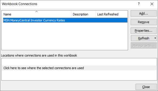
The Workbook Connections dialog box (Select Data > Connections) helps you manage one or more connections to external data sources in your workbook.
You can use this dialog box to do the following:
-
Create, edit, refresh, and delete connections that are in use in the workbook.
-
Verify where external data is coming from, because, for example, the connection was defined by another user.
-
Show where each connection is used in the current workbook.
-
Diagnose an error message about connections to external data.
-
Redirect a connection to a different server or data source, or replace the connection file for an existing connection.
-
Display the Existing Connections dialog box to create new connections. For more information, see Connect to (Import) external data.
-
Display the Connection Properties dialog box to modify data connection properties, edit queries, and change parameters. For more information, see Connection properties.
-
Make it easy to create and share connection files with users.
To manage the connections in the current workbook, do one or more of the following:
Identify a connection
In the top portion of the dialog box, all connections in the workbook are displayed automatically with the following information:
|
Column |
Comment |
|---|---|
|
Name |
The name of the connection, defined in the Connection Properties dialog box. |
|
Description |
An optional description of the connection, defined in the Connection Properties dialog box. |
|
Last refreshed |
The date and time that the connection was last successfully refreshed. If blank, then the connection has never been refreshed. |
Add a connection
-
Click Add to display the Existing Connections dialog box. For more information, see Connect to (Import) external data.
Display connection information
-
Select a connection, and then click Properties to display the Connection Properties dialog box. For more information, see Connection properties.
Refresh the external data
-
Click the arrow next to Refresh, and then do one of the following:
-
To refresh specific connections, select one or more connections, and then click Refresh.
-
To refresh all connections in the workbook, clear all connections, and then click Refresh All.
-
To get status information about a refresh operation, select one or more connections, and then click Refresh Status.
-
To stop the current refresh operation, click Cancel Refresh.
-
For more information, see Refresh an external data connection in Excel.
Remove one or more connections
-
Select one or more connections to be removed from the workbook, and then click Remove.
Notes:
-
This button is disabled when the workbook is protected or an object, such as a PivotTable report, that uses the connection is protected.
-
Removing a connection only removes the connection and does not remove any object or data from the workbook.
-
Important: Removing a connection breaks the connection to the data source and may cause unintended consequences, such as different formula results and possible problems with other Excel features.
Display the locations of one or more connections in the workbook
-
Select one or more connections, and then under Locations where connections are used in this workbook, click the link Click here to see where the selected connections are used.
The following information is displayed.
|
Column |
Comment |
|---|---|
|
Sheet |
The worksheet where the connection is used. |
|
Name |
The Excel query name. |
|
Location |
The reference to a cell, range, or object. |
|
Value |
The value of a cell, or blank for a range of cells. |
|
Formula |
The formula of a cell, or for a range of cells. |
Selecting another connection at the top of the dialog box clears the display of the current information.
See Also
Power Query for Excel Help
Need more help?
Want more options?
Explore subscription benefits, browse training courses, learn how to secure your device, and more.
Communities help you ask and answer questions, give feedback, and hear from experts with rich knowledge.
You all must have heard of Excel Workbook Connections but do know how to manage workbook connection in Excel? Well if you are not having any idea of enabling data connection in Excel workbook.
In that case our, this Excel workbook connections tutorial will help in grabbing every pinch of information reading this. So, that any Excel user can easily perform and manage external data connections in Excel.
What Is Data Connection In Excel?

Data of any Excel workbook can only be bring from different locations. Firstly, either the data is directly stored in your Excel workbook. Or secondly it may be saved in the external data source, like a database, an OLAP (Online Analytical Processing cube) or text file.
Using the data connection in Excel, external data sources are well connected with Excel workbook. Basically this data connection in Excel contains set of information about how to log in, query, locate, and perfectly access the external data source.
After connecting your excel workbook with external data source. One can easily use the refresh option to extract the updated data from their workbook. Using this way, user can get the most updated version of their data including the changes made in the data since it was last refreshed.
Well the Connection information can be stored in a connection file or in the workbook like Universal Data Connection (UDC) file (.udcx) or Office Data Connection (ODC) file (.odc)
These connection files are very useful to share connections on regular basis also to facilitate data source administration.
If you are using the connection file for connecting with the data source. Then in that case Excel will copies down the connection details from the connection file into your Excel workbook.
Different Ways To Perform Excel Workbook Connections

In this Excel workbook connections tutorial we will learn 3 different ways to use Data Connection In Excel 2010/2013/2016/2019:
- Workbook Connections dialog box
- Creating an Office Data Connection (ODC) file (.odc)
- Refresh external data connection
Method 1: Excel Workbook Connections Using Workbook Connections Dialog Box
![]()
Excel Workbook Connections dialog box option helps in easy managing of single or multiple connections with the external data sources of your workbook. Apart from this the Workbook Connections dialog box is helpful to perform the following tasks:
- It helps to edit, refresh, create and delete connections which are used in Excel workbook.
- Show the location of each connection that is already been used in the current Excel workbook.
- Easy diagnosis of error message regarding external data connections.
- With this option, user can either redirect connection to different data or to the different server. Or alternatively user can easily replace the connection file with the existing connection.
- It becomes too easy to make & share connection files.
Steps To Manage Excel Workbook Connection Using Workbook Connections Dialog Box
Here is how to manage connections in your current using Excel workbook i.e by using Workbook Connections dialog box:
Identify a connection
In the top portion of the dialog box, all connections in the workbook are displayed automatically with the following information:
| Column | Comment |
| Name | connection name is, defined within Connection Properties dialog box. |
| Description | A short description about connection, is mentioned in Connection Properties dialog box. |
| Last refreshed | when was the connection was last refreshed such as it’s date and time appears in this section. If it is blank, then it means that the connection has not refreshed yet. |
Add a connection
- Tap to the Add option to get the dialog box of Existing Connections.
Display Connection Information
- For this you need to choose a connection from the opened Existing Connections dialog box.
- Now hit the Properties option and this will open the dialog box of Connection Properties.
Refresh The External Data.
- Hit the arrow option present next to the Refresh option. After then perform anyone of the following:
- If you want to refresh any specific connections only, then make selections of those connections. After then tap to the Refresh option.
- For refreshing all connections of your workbook, just clear off all the connections. After that tap to the Refresh All option.
- If you want to get the status information about refresh operation then choose the connections about which you want to extract information. After then hit on the Refresh Status option.
- For stopping down the current running refresh operation just tap to the Cancel Refresh option.
Remove One Or More Connections
- Choose the connections which you wants to remove from your Excel workbook. After then tap to the Remove option.
Notes:
- Well this option appears disabled to you if your workbook is protected one or if it is an object, like PivotTable report, which uses the protected connection.
- Removing connection will only deletes off the connection. It will not remove any data or any object from your Excel workbook.
Important: By removing connection you are actually breaking the connection with the data source which may leads to cause unintentional consequences, Like different formula results or you may face difficulty in accessing Excel features.
Method 2: Excel Workbook Connections Using Refresh External Data Connection Option

User can connect their Excel workbook with an external data source, like to another Excel workbook, SQL Server database or an OLAP cube.
Well this connection information gets displayed on your workbook as PivotTable report, PivotChart, table.
For keeping the data of your Excel workbook updated you can make use of “Refresh” option to link the data with its source.
So whenever you will refresh your connection, you will only get the most current updated data.
Step To Use Refresh External Data Connection Option
For connections just tap to any cell of your Excel table which uses the connection. After then perform any of the following operation:
- Automatically refresh data when excel workbook is opened
- Automatically refresh data at regular interval
Step To Automatically Refresh Data When Excel Workbook Is Opened
- Tap to the cell present within the external data range.
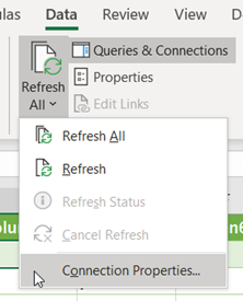
- Now on the Data tab, go to the Queries & Connections Hit the arrow key present within the Refresh All option, and from this tap to the Connection Properties.

- From the opened dialog box of Connection Properties dialog tap to the Usage tab, within Refresh control. After then choose the check box “Refresh data when opening the file”.
- In order to save your workbook with the complete query definition excluding external data. You need to choose the check box “Remove data from the external data range before saving the workbook”.
Step To Automatically refresh data at regular interval:
- Tap to the cell present within the external data range.
- Now on the Data tab, go to the Queries & Connections Hit the arrow key present within the Refresh All option, and from this tap to the Connection Properties.
- In the opened Connection Properties dialog box. Hit Usage tab option.
- Choose the check box Refresh every. After then set the minute interval that will automatically refresh your data after certain period of time.
Method 3: Excel Workbook Connections By Creating An Office Data Connection (ODC) File

By making use of the Data Connection Wizard or Connection Properties dialog box one can easily use their Excel worksheet to create an Office Data Connection (ODC) file (.odc).
- You can perform any of the following task:
- Make new connection with data source. To catch more information, have a look at following topics :
- Connect to SQL Server Analysis Services Database (Import)
- Import or export text files
- Move data from Excel to Access
- Make new connection with data source. To catch more information, have a look at following topics :
- Or you can just make use of the existing connection. For more information, see Connect to (Import) external data.
- After then save the connection detail into the connection file. For this, just make a tap to the Export Connection File option present on the Definition tab of Connection Properties dialog box. This will open the File Save dialog box, so save your current connection information into the ODC file.
Wrap Up:
Hopefully, all the above mentioned fixes to setup Excel Workbook Connections will help you in easy using of data connection in your respective Excel 2010/2013/2016/2019 application. Apart from this if you you have any other query to ask then, ask it in our comment section.


Priyanka is an entrepreneur & content marketing expert. She writes tech blogs and has expertise in MS Office, Excel, and other tech subjects. Her distinctive art of presenting tech information in the easy-to-understand language is very impressive. When not writing, she loves unplanned travels.
Содержание
- Create a relationship between tables in Excel
- More about relationships between tables in Excel
- Notes about relationships
- Example: Relating time intelligence data to airline flight data
- “Relationships between tables may be needed”
- Step 1: Determine which tables to specify in the relationship
- Step 2: Find columns that can be used to create a path from one table to the next
- Create, edit, and manage connections to external data
Create a relationship between tables in Excel
Have you ever used VLOOKUP to bring a column from one table into another table? Now that Excel has a built-in Data Model, VLOOKUP is obsolete. You can create a relationship between two tables of data, based on matching data in each table. Then you can create Power View sheets and build PivotTables and other reports with fields from each table, even when the tables are from different sources. For example, if you have customer sales data, you might want to import and relate time intelligence data to analyze sales patterns by year and month.
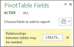
All the tables in a workbook are listed in the PivotTable and Power View Fields lists.

When you import related tables from a relational database, Excel can often create those relationships in the Data Model it’s building behind the scenes. For all other cases, you’ll need to create relationships manually.
Make sure the workbook contains at least two tables, and that each table has a column that can be mapped to a column in another table.
Do one of the following: Format the data as a table, or Import external data as a table in a new worksheet.
Give each table a meaningful name: In Table Tools, click Design > Table Name > enter a name.
Verify the column in one of the tables has unique data values with no duplicates. Excel can only create the relationship if one column contains unique values.
For example, to relate customer sales with time intelligence, both tables must include dates in the same format (for example, 1/1/2012), and at least one table (time intelligence) lists each date just once within the column.
Click Data > Relationships.
If Relationships is grayed out, your workbook contains only one table.
In the Manage Relationships box, click New.
In the Create Relationship box, click the arrow for Table, and select a table from the list. In a one-to-many relationship, this table should be on the many side. Using our customer and time intelligence example, you would choose the customer sales table first, because many sales are likely to occur on any given day.
For Column (Foreign), select the column that contains the data that is related to Related Column (Primary). For example, if you had a date column in both tables, you would choose that column now.
For Related Table, select a table that has at least one column of data that is related to the table you just selected for Table.
For Related Column (Primary), select a column that has unique values that match the values in the column you selected for Column.
More about relationships between tables in Excel
Notes about relationships
You’ll know whether a relationship exists when you drag fields from different tables onto the PivotTable Fields list. If you aren’t prompted to create a relationship, Excel already has the relationship information it needs to relate the data.
Creating relationships is similar to using VLOOKUPs: you need columns containing matching data so that Excel can cross-reference rows in one table with those of another table. In the time intelligence example, the Customer table would need to have date values that also exist in a time intelligence table.
In a data model, table relationships can be one-to-one (each passenger has one boarding pass) or one-to-many (each flight has many passengers), but not many-to-many. Many-to-many relationships result in circular dependency errors, such as “A circular dependency was detected.” This error will occur if you make a direct connection between two tables that are many-to-many, or indirect connections (a chain of table relationships that are one-to-many within each relationship, but many-to-many when viewed end to end. Read more about Relationships between tables in a Data Model.
The data types in the two columns must be compatible. See Data types in Excel Data Models for details.
Other ways to create relationships might be more intuitive, especially if you are not sure which columns to use. See Create a relationship in Diagram View in Power Pivot.
Example: Relating time intelligence data to airline flight data
You can learn about both table relationships and time intelligence using free data on the Microsoft Azure Marketplace. Some of these datasets are very large, requiring a fast internet connection to complete the data download in a reasonable period of time.
Click Get External Data > From Data Service > From Microsoft Azure Marketplace. The Microsoft Azure Marketplace home page opens in the Table Import Wizard.
Under Price, click Free.
Under Category, click Science & Statistics.
Find DateStream and click Subscribe.
Enter your Microsoft account and click Sign in. A preview of the data should appear in the window.
Scroll to the bottom and click Select Query.
Choose BasicCalendarUS and then click Finish to import the data. Over a fast internet connection, import should take about a minute. When finished, you should see a status report of 73,414 rows transferred. Click Close.
Click Get External Data > From Data Service > From Microsoft Azure Marketplace to import a second dataset.
Under Type, click Data.
Under Price, click Free.
Find US Air Carrier Flight Delays and click Select.
Scroll to the bottom and click Select Query.
Click Finish to import the data. Over a fast internet connection, this can take 15 minutes to import. When finished, you should see a status report of 2,427,284 rows transferred. Click Close. You should now have two tables in the data model. To relate them, we’ll need compatible columns in each table.
Notice that the DateKey in BasicCalendarUS is in the format 1/1/2012 12:00:00 AM. The On_Time_Performance table also has a datetime column, FlightDate, whose values are specified in the same format: 1/1/2012 12:00:00 AM. The two columns contain matching data, of the same data type, and at least one of the columns ( DateKey) contains only unique values. In the next several steps, you’ll use these columns to relate the tables.
In the Power Pivot window, click PivotTable to create a PivotTable in a new or existing worksheet.
In the Field List, expand On_Time_Performance and click ArrDelayMinutes to add it to the Values area. In the PivotTable, you should see the total amount of time flights were delayed, as measured in minutes.
Expand BasicCalendarUS and click MonthInCalendar to add it to the Rows area.
Notice that the PivotTable now lists months, but the sum total of minutes is the same for every month. Repeating, identical values indicate a relationship is needed.
In the Field List, in “Relationships between tables may be needed”, click Create.
In Related Table, select On_Time_Performance and in Related Column (Primary) choose FlightDate.
In Table, select BasicCalendarUS and in Column (Foreign) choose DateKey. Click OK to create the relationship.
Notice that the sum of minutes delayed now varies for each month.
In BasicCalendarUS and drag YearKey to the Rows area, above MonthInCalendar.
You can now slice arrival delays by year and month, or other values in the calendar.
Tips: By default, months are listed in alphabetical order. Using the Power Pivot add-in, you can change the sort so that months appear in chronological order.
Make sure that the BasicCalendarUS table is open in the Power Pivot window.
On the Home table, click Sort by Column.
In Sort, choose MonthInCalendar
In By, choose MonthOfYear.
The PivotTable now sorts each month-year combination (October 2011, November 2011) by the month number within a year (10, 11). Changing the sort order is easy because the DateStream feed provides all of the necessary columns to make this scenario work. If you’re using a different time intelligence table, your step will be different.
“Relationships between tables may be needed”
As you add fields to a PivotTable, you’ll be informed if a table relationship is required to make sense of the fields you selected in the PivotTable.
Although Excel can tell you when a relationship is needed, it can’t tell you which tables and columns to use, or whether a table relationship is even possible. Try following these steps to get the answers you need.
Step 1: Determine which tables to specify in the relationship
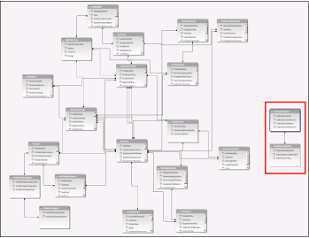
If your model contains just a few tables, it might be immediately obvious which ones you need to use. But for larger models, you could probably use some help. One approach is to use Diagram View in the Power Pivot add-in. Diagram View provides a visual representation of all the tables in the Data Model. Using Diagram View, you can quickly determine which tables are separate from the rest of the model.
Note: It’s possible to create ambiguous relationships that are invalid when used in a PivotTable or Power View report. Suppose all of your tables are related in some way to other tables in the model, but when you try to combine fields from different tables, you get the “Relationships between tables may be needed” message. The most likely cause is that you’ve run into a many-to-many relationship. If you follow the chain of table relationships that connect to the tables you want to use, you will probably discover that you have two or more one-to-many table relationships. There is no easy workaround that works for every situation, but you might try creating calculated columns to consolidate the columns you want to use into one table.
Step 2: Find columns that can be used to create a path from one table to the next
After you’ve identified which table is disconnected from the rest of the model, review its columns to determine whether another column, elsewhere in the model, contains matching values.
For example, suppose you have a model that contains product sales by territory, and that you subsequently import demographic data to find out if there is correlation between sales and demographic trends in each territory. Because the demographic data comes from a different data source, its tables are initially isolated from the rest of the model. To integrate the demographic data with the rest of your model, you’ll need to find a column in one of the demographic tables that corresponds to one you’re already using. For example if the demographic data is organized by region, and your sales data specifies which region the sale occurred, you could relate the two datasets by finding a common column, such as a State, Zip code, or Region, to provide the lookup.
Besides matching values, there are a few additional requirements for creating a relationship:
Data values in the lookup column must be unique. In other words, the column can’t contain duplicates. In a Data Model, nulls and empty strings are equivalent to a blank, which is a distinct data value. This means that you can’t have multiple nulls in the lookup column.
Data types of both the source column and lookup column must be compatible. For more information about data types, see Data types in Data Models.
To learn more about table relationships, see Relationships between tables in a Data Model.
Источник
Create, edit, and manage connections to external data
You can use Excel to create and edit connections to external data sources that are stored in a workbook or in a connection file. You can easily manage these connections, including creating, editing, and deleting them using the current Queries & Connections pane or the Workbook Connections dialog box (available in previous versions).
Note: Connections to external data may be currently disabled on your computer. To connect to data when you open a workbook, you must enable data connections by using the Trust Center bar, or by putting the workbook in a trusted location. For more information, see Add, remove, or modify a trusted location for your files, Add, remove, or view a trusted publisher, and View my options and settings in the Trust Center.
Data in an Excel workbook can come from two different locations. The data may be stored directly in the workbook, or it may be stored in an external data source, such as a text file, a database, or an Online Analytical Processing (OLAP) cube. The external data source is connected to the workbook through a data connection, which is a set of information that describes how to locate, log in, query, and access the external data source.
When you are connected to an external data source, you can also perform a refresh operation to retrieve the updated data. Each time that you refresh data, you see the most recent version of the data, including any changes that were made to the data since it was last refreshed.
Connection information can either be stored in the workbook or in a connection file, such as an Office Data Connection (ODC) file (.odc) or a Universal Data Connection (UDC) file (.udcx). Connection files are particularly useful for sharing connections on a consistent basis and for facilitating data source administration.
If you use a connection file to connect to a data source, Excel copies the connection information from the connection file into the Excel workbook. When you make changes by using the Connection Properties dialog box, you are editing the data connection information that is stored in the current Excel workbook, and not the original data connection file that may have been used to create the connection, indicated by the file name that is displayed in the Connection File property. Once you edit the connection information (with the exception of the Connection Name and Connection Description properties), the link to the connection file is removed and the Connection File property is cleared.
By using the Connection Properties dialog box or the Data Connection Wizard, you can use Excel to create an Office Data Connection (ODC) file (.odc). For more information, see Connection properties and Share data with ODC.
Do one of the following:
Use an existing connection. For more information, see Connect to (Import) external data.
Save the connection information to a connection file by clicking Export Connection File on the Definition tab of the Connection Properties dialog box to display the File Save dialog box, and then save the current connection information to an ODC file.
Note The Queries & Connections pane is available in Microsoft Office 365 for Excel and Excel stand-alone version 2019 or later. It replaced the Workbook Connections dialog box which is available in Excel stand-alone versions 2010, 2013, and 2016.
The Queries & Connections pane (Select Data > Queries & Connections) In one location, you can get to all the information and commands you need to work with your external data. This pane has two tabs:
Queries Displays all the queries in the workbook. Right click a query to see available commands. For more information, see Manage queries.
Connections Displays all the connections in the workbook. Right click a connection to see available commands. For more information, see Connection properties.
Note The Workbook Connections dialog box is available in Excel stand-alone versions 2010, 2013, and 2016, but was replaced in Microsoft Office 365 for Excel and Excel stand-alone version 2019 with the Queries & Connections pane.
The Workbook Connections dialog box (Select Data > Connections) helps you manage one or more connections to external data sources in your workbook.
You can use this dialog box to do the following:
Create, edit, refresh, and delete connections that are in use in the workbook.
Verify where external data is coming from, because, for example, the connection was defined by another user.
Show where each connection is used in the current workbook.
Diagnose an error message about connections to external data.
Redirect a connection to a different server or data source, or replace the connection file for an existing connection.
Display the Existing Connections dialog box to create new connections. For more information, see Connect to (Import) external data.
Display the Connection Properties dialog box to modify data connection properties, edit queries, and change parameters. For more information, see Connection properties.
Make it easy to create and share connection files with users.
To manage the connections in the current workbook, do one or more of the following:
Identify a connection
In the top portion of the dialog box, all connections in the workbook are displayed automatically with the following information:
The name of the connection, defined in the Connection Properties dialog box.
An optional description of the connection, defined in the Connection Properties dialog box.
The date and time that the connection was last successfully refreshed. If blank, then the connection has never been refreshed.
Add a connection
Click Add to display the Existing Connections dialog box. For more information, see Connect to (Import) external data.
Display connection information
Select a connection, and then click Properties to display the Connection Properties dialog box. For more information, see Connection properties.
Refresh the external data
Click the arrow next to Refresh, and then do one of the following:
To refresh specific connections, select one or more connections, and then click Refresh.
To refresh all connections in the workbook, clear all connections, and then click Refresh All.
To get status information about a refresh operation, select one or more connections, and then click Refresh Status.
To stop the current refresh operation, click Cancel Refresh.
Remove one or more connections
Select one or more connections to be removed from the workbook, and then click Remove.
This button is disabled when the workbook is protected or an object, such as a PivotTable report, that uses the connection is protected.
Removing a connection only removes the connection and does not remove any object or data from the workbook.
Important: Removing a connection breaks the connection to the data source and may cause unintended consequences, such as different formula results and possible problems with other Excel features.
Display the locations of one or more connections in the workbook
Select one or more connections, and then under Locations where connections are used in this workbook, click the link Click here to see where the selected connections are used.
The following information is displayed.
The worksheet where the connection is used.
The Excel query name.
The reference to a cell, range, or object.
The value of a cell, or blank for a range of cells.
The formula of a cell, or for a range of cells.
Selecting another connection at the top of the dialog box clears the display of the current information.
Источник
Microsoft Query allows you use SQL directly in Microsoft Excel, treating Sheets as tables against which you can run Select statements with JOINs, UNIONs and more. Often Microsoft Query statements will be more efficient than Excel formulas or a VBA Macro.
Contents
- 1 What is query function in Excel?
- 2 Where are query options in Excel?
- 3 What is the difference between queries and connections in Excel?
- 4 How do you query text in Excel?
- 5 What is a query in a database?
- 6 How do you create a query?
- 7 How do I remove a query in Excel?
- 8 How do I open a query in Excel?
- 9 How do I create a workbook in Excel?
- 10 How do I know if I have power query in Excel?
- 11 Where is power query?
- 12 What is a query in access?
- 13 How write SQL query in Excel?
- 14 What is Excel Vlookup?
- 15 What is query give an example?
- 16 What are examples of queries?
- 17 What is a query in computer?
- 18 What is query design?
- 19 What is a query form?
- 20 What are workbook connections in Excel?
What is query function in Excel?
Power Query is a business intelligence tool available in Excel that allows you to import data from many different sources and then clean, transform and reshape your data as needed.It allows you to set up a query once and then reuse it with a simple refresh.
Where are query options in Excel?
To display the Query Options dialog box: Power Query Editor Select File > Options and settings > Query options. Excel Select Data > Get Data > Query Options.
What is the difference between queries and connections in Excel?
Edit: Let’s put it this way: The connection is just that. It connects your workbook to a data source. Like a highway connecting two cities. A query is the request for actual data that you spell out, calling from your workbook (via the connection) into the data source.
How do you query text in Excel?
Create a simple formula
In the POWER QUERY ribbon tab, choose From Other Sources > Blank Query. In the Query Editor formula bar, type = Text. Proper(“text value”), and press Enter or choose the Enter icon. Power Query shows you the results in the formula results pane.
What is a query in a database?
A query can either be a request for data results from your database or for action on the data, or for both. A query can give you an answer to a simple question, perform calculations, combine data from different tables, add, change, or delete data from a database.
How do you create a query?
On the Create tab, in the Queries group, click Query Wizard. In the New Query dialog box, click Simple Query Wizard, and then click OK. Next, you add fields. You can add up to 255 fields from as many as 32 tables or queries.
How do I remove a query in Excel?
STEP 1: Let us edit an existing query that we want to modify. Double click on your Query to open the Power Query Editor. Right click on the Step #3 and select Delete Until End. STEP 3: Click Delete.
How do I open a query in Excel?
To open a saved query from Excel:
- On the Data tab, in the Get External Data group, click From Other Sources, and then click From Microsoft Query. The Choose Data Source dialog box is displayed.
- In the Choose Data Source dialog box, click the Queries tab.
- Double-click the saved query that you want to open.
How do I create a workbook in Excel?
On the Data tab, click Connections. On the Workbook Connections dialog box, select the connection that you just opened, and then click Properties. On the Connection Properties dialog box, on the Definition tab, select the Always use connection file check box, and then click OK.
How do I know if I have power query in Excel?
You’ll find Power Query in Excel 2016 hidden on the Data tab, in the Get & Transform group. In Excel 2016, the Power Query commands are found in the Get & Transform group on the Data tab. If you’re working with Excel 2010 or Excel 2013, you need to explicitly download and install the Power Query add-in.
Where is power query?
Overview of the Power Query Ribbon
It is now on the Data tab of the Ribbon in the Get & Transform group. In Excel 2010 and 2013 for Windows, Power Query is a free add-in. Once installed, the Power Query tab will be visible in the Excel Ribbon.
What is a query in access?
A query is an Access object used to view, analyze, or modify data. The query design determines the fields and records you see and the sort order.
How write SQL query in Excel?
How to create and run SQL SELECT on Excel tables
- Click the Execute SQL button on the XLTools tab. The editor window will open.
- On the left-hand side find a tree view of all available tables.
- Select entire tables or specific fields.
- Choose whether to place the query output on a new or an existing worksheet.
- Click Run.
What is Excel Vlookup?
VLOOKUP stands for ‘Vertical Lookup’. It is a function that makes Excel search for a certain value in a column (the so called ‘table array’), in order to return a value from a different column in the same row.
What is query give an example?
Query is another word for question. In fact, outside of computing terminology, the words “query” and “question” can be used interchangeably. For example, if you need additional information from someone, you might say, “I have a query for you.” In computing, queries are also used to retrieve information.
What are examples of queries?
Examples of Common Queries
- The Maximum Value for a Column. “What’s the highest item number?”
- The Row Holding the Maximum of a Certain Column.
- Maximum of Column per Group.
- The Rows Holding the Group-Wise Maximum of a Certain Field.
- Using User Variables.
- Using Foreign Keys.
- Searching on Two Keys.
- Calculating Visits per Day.
What is a query in computer?
A query is a question or a request for information expressed in a formal manner. In computer science, a query is essentially the same thing, the only difference is the answer or retrieved information comes from a database.
What is query design?
The query design is a visual representation of the families, fields, and criteria that the query is configured to return.The query design appears you click the Design View link on the Query Tasks menu while you are viewing query results or SQL code.
What is a query form?
A query form means the interface of a search engine. In the form, you place the search terms and choose the operators in order to formulate the query. It is essential to type the search query in a way that the search logic works correctly.
What are workbook connections in Excel?
The Workbook Connections dialog box (Select Data > Connections) helps you manage one or more connections to external data sources in your workbook. You can use this dialog box to do the following: Create, edit, refresh, and delete connections that are in use in the workbook.
How to use external data connections in Excel? Today’s tutorial is all about data import (SQL, CSV, and XML) and the managing of data sources. Stay with us!
It is not surprising that we rarely store databases and a large amount of raw data in Excel worksheets. The main reason for this is that Excel was not made for this.
Use external data connections to build a dashboard, and you have to work with a considerable amount of data. We think that the subject is so important. So, we provide a whole separate article about it.
The most common External Data Connections
The most important data sources are:
- SQL database
- CSV file
- XML
How can we import data using various external data connections into Excel?
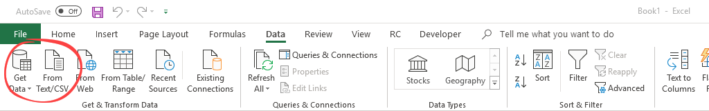
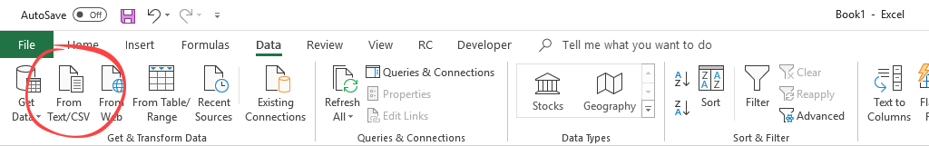
The starting point is always the same. First, go to the Data tab on the ribbon. Then, choose ‘Get data’ or ‘From Text/CSV.’ Then, of course, we can import data with the help of a web query also.
Connect to External Data Sources
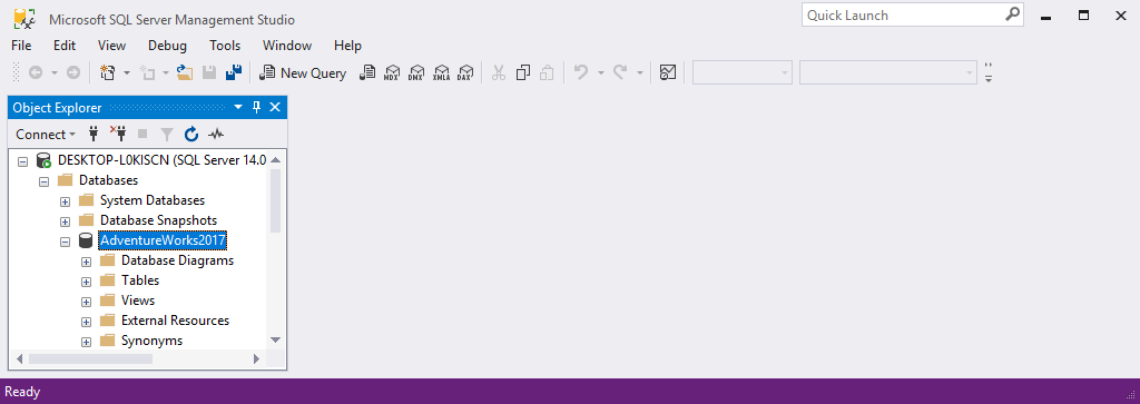
We’ll use the ‘AdventureWorks’ SQL Server database. It’s well known and used by many. SQL Server Management studio will help us import the given database from a backup.
First, start Excel.
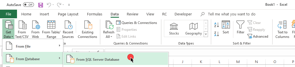
Choose the Get Data > From database > From SQL Server Database menu.
In the next window, we have to give the name of the SQL Server.
The name of the Server is a mandatory field. The name of the database is optional.
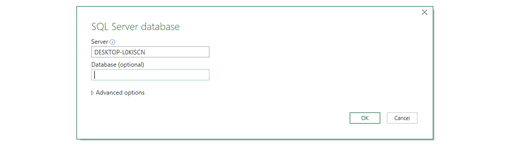
The Navigator will appear by clicking on the OK button, and we can find multiple things here. In our example, we’ll use the AdventureWorks database table.
We want to direct your attention to the ‘Select multiple items’ checkbox. If we do not check it, we can only import one table.
And what happens if we check it? Then we were able to import the highlighted table AND all the relevant connected tables also!
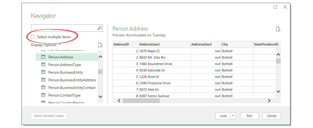
Now we’d like to import the ‘Person.Address’ table.
It can be seen in the figure below. If we need the connected tables also, we have to check the ‘Select related tables’ button, located at the bottom of the window.
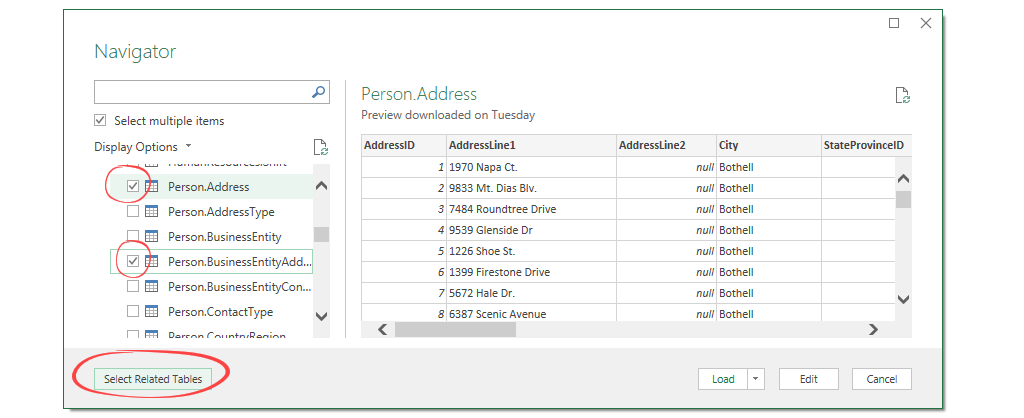
We have highlighted the data.
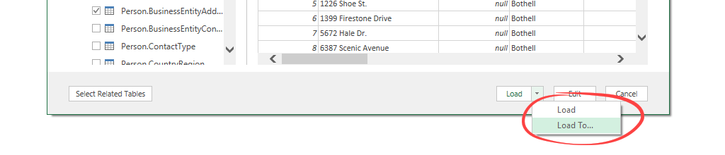
Now we’ll import with the help of the external data source. Then, finally, we’ll transfer the data into Excel by clicking on the Load button.
If we pay more attention to the button, we can see a drop-down list.
Let’s try out how the ‘Load to’ option work!
Take a closer look at the Import Data window!
We can see we have more options for data import. This chapter will show you how to create a data structure.
The Import Data Window: Select views

We can choose a view and layout for our project using the import data window.
- Table: we can display data in tabular form
- Pivot Table Report: we don’t have to specifically explain the advantages of Pivot tables. Choose this if you’d like to group the data in a short time. If you’d like to apply the drill-down method, this is the best choice!
- Pivot Chart: using the columns of the Pivot table, we can make a chart
- Only create a connection: if we don’t need the data right away, then we only create the connection between the SQL database and the Excel worksheet.
- Add this data to Data Model: in this case, the highlighted data will upload into the Power Pivot Data Model.
Explanation of the Get and Transform function: If you use this function in Excel, you create a query in your workbook. This query enables you to manage data using various external data sources. For example, suppose you want to refresh your data and keep your dashboard always-on use, the built-in Data Model in Excel. Of course, the most effective is to use the tabular format. So let’s choose this option!
How to manage and refresh External Data Connections?
We are already done with an important step.
Now we have our data in Excel. What happens when data changes in the source database? How can we keep data up to date? We’ll find the answer in this chapter.
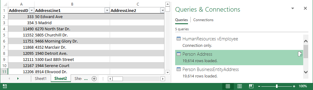
Check the ‘Queries and Connections’ window! It’s located on the right-hand side.
You can see the imported records and all related records of the Person.Address table. Every single database table is on a separate Worksheet.
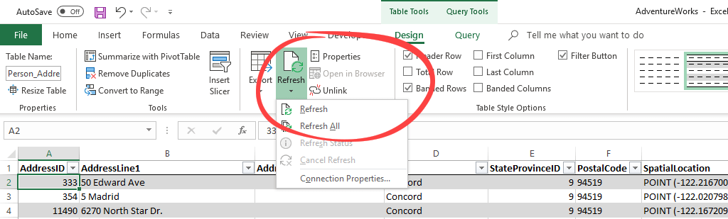
Refreshing Data Connections manually
Usually, we use two methods to refresh existing data connections. First, we can find this menu on the ribbon in the Table Tools tab. Then, click on Refresh / Refresh all icons to refresh the data connections manually.
It is important to note a big difference between the two. We use Refresh when we only want to refresh the data of the given Worksheet. For example, a specific database table. When we use the Refresh all button, every table structure and all the Worksheets are being refreshed.
Using auto-refresh control to Scheduled Data Import
We also have the option to automate this process.
How to schedule refreshing? Set a 10-minute interval and forget about the manual work.
Click on the ‘Existing connections’ icon on the Data tab.
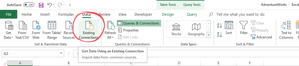
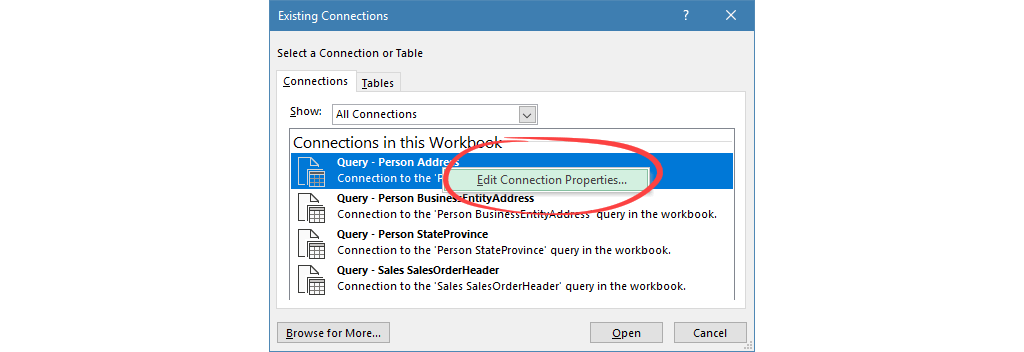
We’ll see the following window appear. We see the relevant connections of the workbook in one list.
After a right-click, you can choose the ‘Edit Connection Properties’ button.
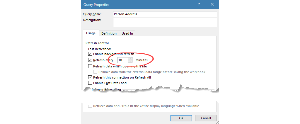
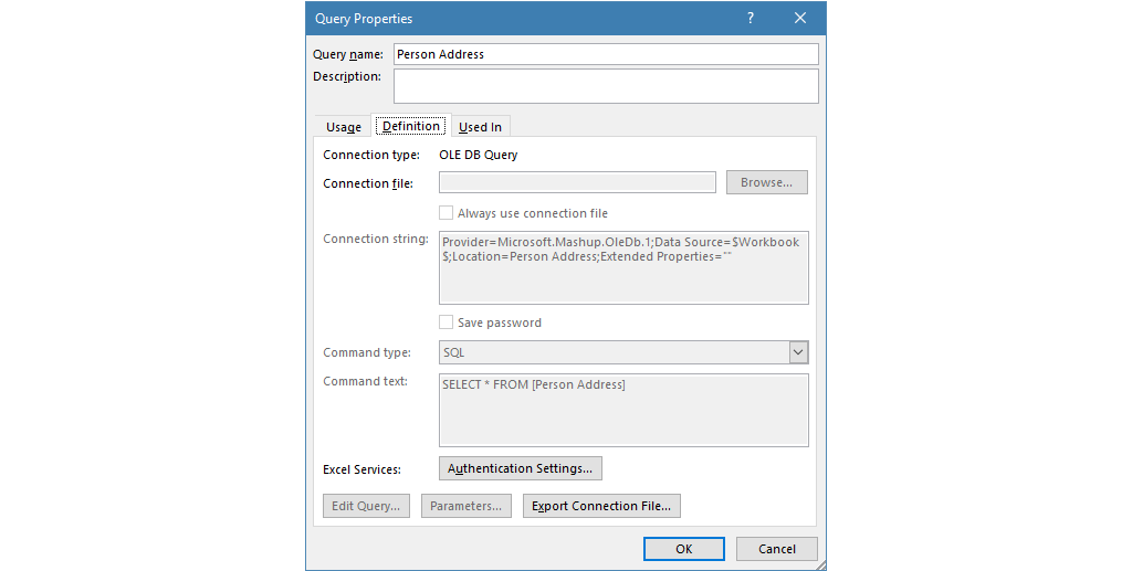
The Query Properties Window
You can find all the adjustments on the ‘Usage’ tab. First, let us set the parameters of the query! Here are the details below:
The Refresh Control section informs us of the actual setups.
- Enable Background refresh: This is a query running in the background. We’ll be informed about the status of the process. Check the marked section on the picture. The extraction is in progress.

- Refresh every x minutes: We can set the intervals of the import. Our data set will be updated using external data sources.
- Refresh Data when opening file: This setting is automatically refreshing the data connection the moment Excel Workbook is opened. Usually, we shouldn’t use this option. If a large query starts up, it can even freeze up Excel. We’re better off if we refresh data after we’ve opened the workbook.
- Refresh This Connection on Refresh All: We already talked about this, but it is very important to let’s see it again! If we allow this option, all imported tables will refresh. (If not, then only the data on the active Worksheet will refresh.)
We can find more information about the data connection on the Definition tab. Add a specific name for the query. In the description field, we can give notes also.
Now let us see further options:
- Connection Type: The type of the connection, in our case, is OLE DB Query.
- Connection file: We can save the connection file to any place we want to. Also, we can browse an already created connection file.
- Connection String: It describes how and what we’ll import using external data sources.
- Command type: In our example, this is SQL.
- Command text: If you want, you can write your own SQL query. In this case, we import all records from the Person.Address table.
Importing CSV files to Excel – External Data Connection Example
In this chapter, we’ll import a CSV file containing sales records into Excel. This will be a lot easier than the SQL data import.
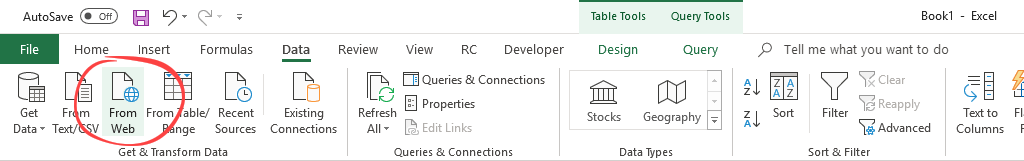
Choose the ‘From text / CSV’ option from the ‘Get and Transform Data’ option on the Data tab.
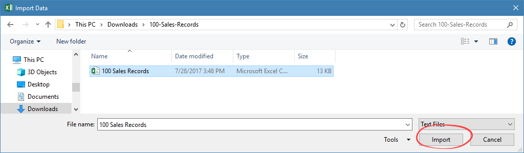
Locate the file and click import.
Before the data import, a preview window will appear. You can set the code page in the ‘File Origin’ section.
In the ‘Delimiter’ menu, you can give the character that will separate the columns of the imported table. The default ‘comma’ setting is the right one for us.
There’s the usual ‘Load / Load To’ button on the bottom right-hand corner. We have talked about this before. The Tabular format is perfect for us now.
Click on the Load button.
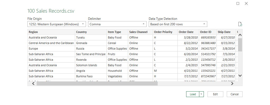
The file containing 100 sales records is in Excel in a matter of moments using external data sources!
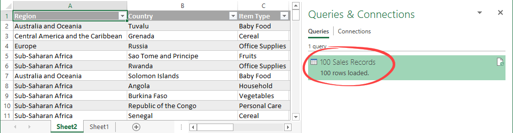
Import Data from Website into Excel using XML files
We have two choices to import from XML to Excel. We either use a specific URL address or browse the file itself.
Using Web query
In this example, we’ll import a short restaurant menu into Excel using a web query.
Type the URL and click OK.

On the left-hand side of the Navigator Window, highlight the table we would like to import. After the highlight on the right-hand side, we’ll see a preview.
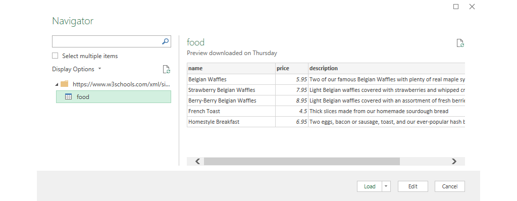
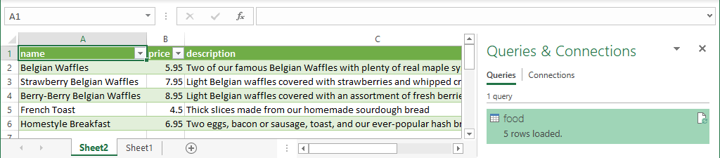
Click on the Load button.
With the help of the external data source, the table’s data will be on the given Worksheet.
Import a local XML file
On the Data Tab, choose Get Data > From file > From XML menu.

Click on the Import button and open the XML file.
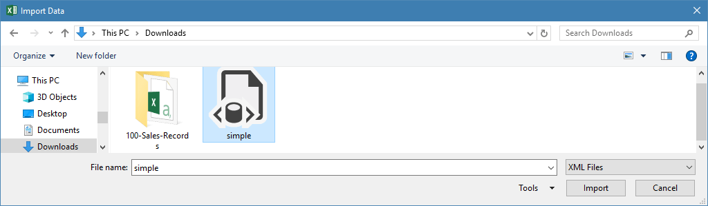
From here on, the steps are entirely the same as described in the web query tutorial.
Conclusion
In today’s article, we endeavored to show you the most critical external data sources. We can choose multiple formats for the data needed to be imported. Last but not least, we talked about the management of data connections. Excel is excellently capable of making charts, reports, and various data visualizations. We should leave the managing of large data to external data sources.
Download the examples!
Working with Excel, a day will come when you’ll need to reference data from one workbook in another one. It’s a common use case and pretty easy to pull off. Join us as we explain how to link two Excel files and discuss many possible scenarios.
How to link Excel files – what are the available options?
Just as there are many different versions of Excel, the ways to link data also differ. It’s a lot easier if you share your Excel files in OneDrive rather than locally but we’ll discuss both scenarios.
Choosing how to link data depends also on the sheer volume of what you wish to link. If we’re talking here about particular cells or a column from your workbook, the default methods will do just fine. If you’re after linking entire Excel files, using tools such as Coupler.io with its Excel integrations may prove to be more efficient. But we’ll get to that!
You can link two or more Excel files stored on your hard drive. When the data changes in a Source file, the change will be quickly reflected in the Destination file.
The drawback of this approach is that it will only work on your local machine. Even if you share both files with another user, the link will cease to exist and they’ll be forced to re-add it. What’s more, the data will be only updated if both files are open at the same time.
So if you have a choice, it’s better to add both files to your OneDrive. If they’re already in there, you may as well jump to the How to link between Cloud-based Excel files section.
To link 2 Excel files stored locally, you have two options:
- Type in a formula referencing the exact location in a Source file
- Copy the desired cells and paste them as a link
How to link between files in desktop Excel?
To reference a single cell in another local file, you’ll use the following formula:
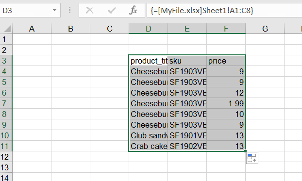
=[SourceWorkbook.xlsx]Sheet1!$A$1
Replace SourceWorkbook.xlsx with the name of the file stored on your machine. Then, point to an exact sheet and a cell. A reference to a range of cells could like this:
=[MyFile.xlsx]Sheet1!A1:C8
Press ENTER to save the formula and pull the data. If you’re on an older version of Excel, you may need to press CTRL+SHIFT+ENTER instead.
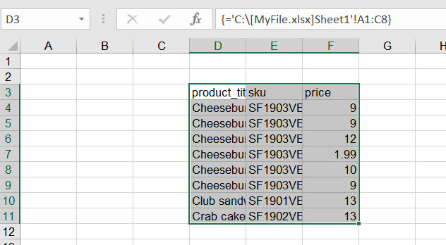
When you close the Source file, the formulas will change to include the entire path of the file – for example:
='C:[MyFile.xlsx]Sheet1'!A1:C8
As an alternative, you can:
- Open a Source file, select the desired cells, and copy them.

- Head back to the Destination file, right-click on a desired cell or cells and choose to paste as a link.

- Here is the result:
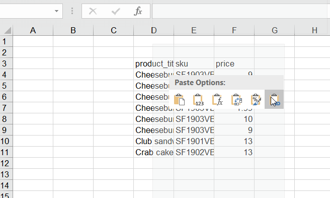
Note that if the Source file is closed, and you reference it with a formula, no data will be pulled until you open a file.
How to link between cloud-based files in Excel?
When you wish to link Excel Online files or use those stored in OneDrive, things become easier. You can freely share files among coworkers and any interlinking won’t be affected. Links in files also refresh in near real time, giving you peace of mind that you’re working with the latest data.
The feature that enables it is called Workbook Links. We’ll explain how it works in the following chapters.
Workbook Links are suitable for individual cells or ranges of them. You may also link individual columns but the more data is involved, the slower your calculations will be. If you’re going to be linking entire worksheets or workbooks, it’s far better to focus on importing, rather than linking them. This is best done with dedicated tools.
There is more on that in the How to link a wide range of cells to Excel or another service chapter.
How to link two Excel files?
Let’s start with a most basic use case – you’re running some operations in your Excel workbook. In one of the fields, you wish to use the value(s) from another workbook and have it update automatically.
The flow is simple:
- In workbook 1 (source), highlight the data you want to link and copy it.
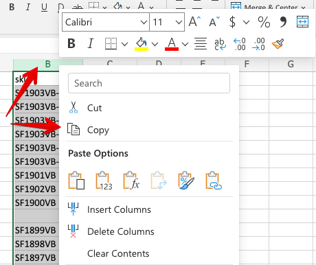
- In workbook 2 (destination), right-click on the first row and select the Link icon.

The latest data will be imported. A yellow bar will, however, appear now as well as every time you open a destination workbook.

To enable the data sync, select Enable Content.
For some more advanced settings, you can choose the Manage Workbook Links button to look up the list of connected workbooks and a status for each – most likely it will be Connection Blocked.
To sync, press the Enable Content button from the yellow bar.

If any errors occur, you’ll see them in the menu to the right. For each of the connected files, you can press the Refresh button to manually pull the latest data. You can also use the button above to refresh data for all your links.
Of course, the whole idea of creating links between workbooks is not to keep refreshing the data manually. Once the data has been refreshed, an option to set automatic updates will be enabled.
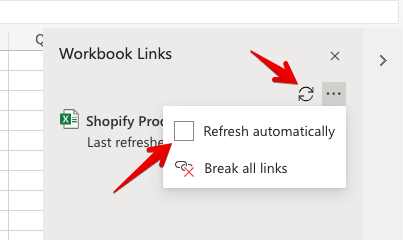
If you tick Refresh automatically, the data will start to refresh periodically.
How to link a wide range of cells to Excel or another service?
The more data you link, the more computing your Excel needs to perform to pull the data and refresh it. It’s not an issue if you have a few or a few dozens of links spread across files.
However, if you wish to regularly pull thousands of cells into your workbooks, it will significantly slow down your workbooks. It may delay the data refresh and may leave you wondering whether the data has already been refreshed or not.
To avoid that, for larger operations it’s better to use tools dedicated to importing data such as Coupler.io. With Coupler.io, you can pull the desired ranges of cells directly into another Excel workbook or worksheet. You can then refresh the data automatically at a chosen schedule.
If you wish to, you can also import the Excel data to other services, such as Google Sheets or Google BigQuery, or bring it to Excel from Airtable, Pipedrive, Hubspot, and many others.
To get started with Coupler.io, create an account, log in, and click the Add an importer button.
From the list of source applications, choose Excel.

Next, click the Connect button. Log in with your Microsoft account and allow for Coupler.io to connect.
Once connected, you’ll need to choose the workbook from your OneDrive that we’ll be importing from. Also select the worksheet in this file.
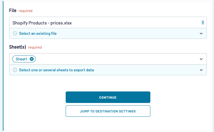
Although it’s optional, most often you’ll want to specify the range of cells to import. If you don’t, all data from a given sheet will be fetched.
You may use the standard Excel formatting and pull, for example, cells C1:D8. You may also pull an entire column by typing, for example, C1:C.

Jumping to the Destination settings, choose where to import the data to. We’ll go with Excel as we just want to move the data from one workbook to another but there are other options available too.
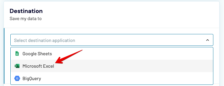
If you’re importing from Excel to Excel, there’s no need to connect your account again, unless you’re importing to someone else’s account. Select it, and specify the exact destination.
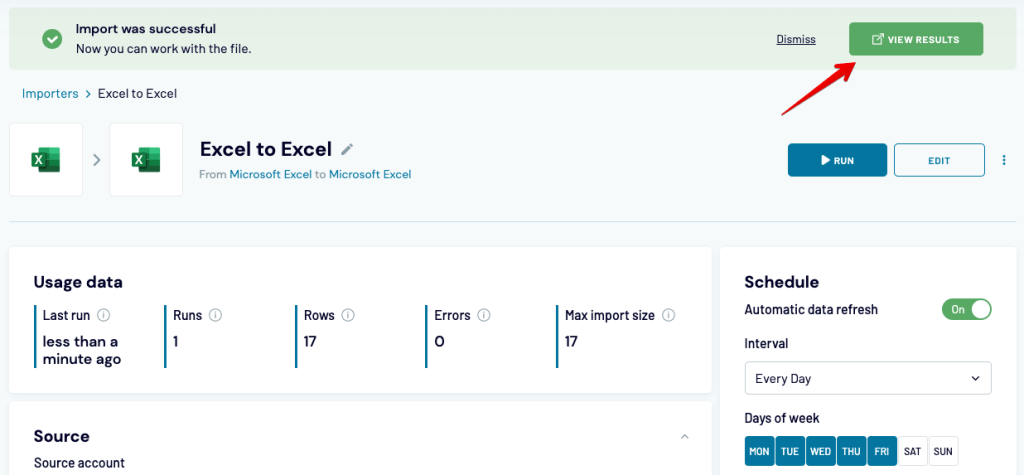
Finally, you can create a schedule for when the data should be imported. Choose what works best for you and run the importer.

Give it a little while to load, and then open the destination worksheet to see the results.
How to link Excel files and sync in real-time?
One of the advantages of using Excel files stored on OneDrive is their ability to sync data between one another. Microsoft advertises it as real-time sync but after some tests, we would call it a near real time.
If you’re used to the refresh rate of Google Sheets, for example, you may be disappointed. However, in most situations, a slight delay won’t cause any trouble.
To link files in Excel, follow the steps we outlined in the How to link Excel files chapter.
When data is changed in the destination file, most likely you won’t see an update visible right away in the source file. If you do nothing about it and just move on to the next task, you should see a refreshed number in a cell in a few minutes’ time. It will then continue refreshing at regular intervals.
If you want to speed things up, you can run an instant refresh by clicking Data -> Workbook Links in the menu and then the icon to refresh the data from a particular workbook.

This will often work, but only if the data in the source workbook has already been saved. Once again, it doesn’t happen instantly but only at regular (quite frequent) intervals.
If you’re anxious to have the data refreshed presently, you may consider refreshing the source file after making a change. This will prompt an automatic save. After that, manually force a data refresh in the destination file and it will fetch the latest saved data.
As a reminder, if you use Coupler.io to import data from one Excel workbook to another, you decide on the refresh schedule. For some, morning sync from Monday to Friday will do just fine. Others will prefer more frequent syncs – with Coupler.io you can even do it every 15 minutes.
FAQ: How to link Excel files
Let’s now discuss some specific use cases for how to link files in Excel. The tips below apply for files stored in OneDrive. If you only use Excel locally, jump back to the How to link local files in Excel section.
How to link cells in different Excel files?
For linking individual cells across files, the procedure is very much the same as we discussed earlier:
- Highlight the cell you want to reuse elsewhere and copy it.
- Right-click on the desired destination and select the Link icon from the Paste Options section.
If you’re importing to the same workbook as before, you won’t need to Enable Content again. If you reloaded it in the meantime, or are just linking the data to a new workbook, choose Manage Workbook Links and then Enable Content from the same bar.
Note that if you link multiple sets of cells or data ranges from the same workbook serving as a Source, they will all appear as a single position on your list of Workbook Links.
In the example below, you can see the data we imported from our sample Shopify store using Coupler.io.
We have a range of prices to the left linked from the respective workbook. Below there’s also a name of one of our products linked from another place in the same workbook. To the right, we can refresh data for all linked fields or, for example, enable automatic data refreshes.

How to link two Excel files without opening the source file?
You can link files in Excel without actually opening the source file. Of course, you’ll need to know the exact location of the cell or range of cells you wish to link. What’s more, to link Excel Online files or anything else stored on your OneDrive, you’ll need to fetch your unique ID.
To do so, set up a link in the traditional way we described above. Then, click on any linked cell in the Destination file and check its formula. It will look something like this:
='https://d.docs.live.net/18644c626caae38c/[myworkbook1.xlsx]Sheet1'!$C$2
The ID will follow right after the live.net link:

To insert a link from any given workbook, copy the formula with your ID and swap the file name and the cell range with the right values. Press ENTER and the latest data will be fetched.
How to link Excel columns between files?
Choosing a range of cells limits you to only the values currently present in the Source workbook. If anything new appears, it won’t be linked and, as such, won’t appear in the Destination workbook.
The solution is often to link an entire column and reference it in another file. To do so, click on any column in the Source file and copy it.
Then, select the first row of a column you want to add a link to and choose the Link icon. All the rows from the chosen column will be imported.

Rather than click, you can also enter the formulas directly. To link an entire column, it’s best to link to the first cell and then stretch the formula to the other rows.
When you insert the formula for the first row, be sure to remove the second $ (dollar) sign pointing to the specific cell. So, instead of the reference:
(...)Sheet1'!$C$2
Make it:
(...)Sheet1'!$C2
How to link fields between multiple files in Excel?
Advanced calculations may require referencing data from multiple spreadsheets at the same time. In the same way, the calculated data can then be referenced in other workbooks, creating a complex network of interconnected links.
As you recall from the earlier chapters, the formulas for linking cells between Excel Online files look somewhat like this:
='https://d.docs.live.net/18373e637ca3e48c/[Shopify Products - prices.xlsx]Sheet1'!$C$8
For the purpose of running any calculations or just adjusting the formulas as we go, the link is far too complex. It’s much better to link the desired fields into the destination workbook and then reference them from another worksheet in the same workbook.
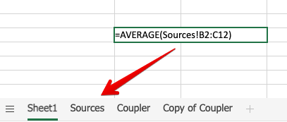
To do so, create a separate worksheet in your destination file where you’ll link all the external data. Name it accordingly – for example, “Sources”. Link the desired data by copying it from the source file and then pasting it as links (just as we did before).
Then, jump to the worksheet in the destination file. To reference the data from another sheet, use the following pattern:
Sheet_name!$A$1
For example, for calculating the average value of a range of cells present now in another worksheet, we would use:
=AVERAGE(Sources!B2:B12)
You can also type in the “=” sign (plus optionally a function name) and then jump to another worksheet and highlight the arguments. Press ENTER and the formula will be resolved.
In the standard version of Excel, the approach is pretty much the same, just with some small changes in the syntax of the links, as we mentioned earlier.
How to link Excel files – summing up
Linking Excel files can save you plenty of time and help you automate many dull processes.
It can also make things harder if you begin to link from one file to another, then to another, and another. The more interconnected workbooks become, the more complex it will be to troubleshoot the entire flow.
Find the right balance and use the right methods for linking your data.
When moving individual cells or ranges of them, Workbook Links work perfectly and are very easy to set up.
For moving large sets of data between workbooks or linking entire files, it’s a lot better to use tools such as Coupler.io. You’ll be able to set up your own schedule for imports, and all data transfers will happen outside of Excel. As a result, no Excel resources will be used, and you’ll be able to work much more smoothly while the information is synced in the background.
Thanks for reading!
-

Technical Content Writer on Coupler.io who loves working with data, writing about it, and even producing videos about it. I’ve worked at startups and product companies, writing content for technical audiences of all sorts. You’ll often see me cycling🚴🏼♂️, backpacking around the world🌎, and playing heavy board games.

Back to Blog
Focus on your business
goals while we take care of your data!
Try Coupler.io
Last Update: Jan 03, 2023
This is a question our experts keep getting from time to time. Now, we have got the complete detailed explanation and answer for everyone, who is interested!
Asked by: Delia Swift MD
Score: 4.9/5
(20 votes)
To open the Existing Connections dialog box, select Data > Existing Connections. You can display all the connections available to you and Excel tables in your workbook. You can open a connection or table from the list and then use the Import Data dialog box to decide how you want to import the data.
How do I change an existing connection in Excel?
Manually Editing Data Connections in Excel
- Go to the Data tab on the Ribbon and select Connections. …
- Choose the connection you want to edit and then click the Properties button.
- The Connection Properties dialog box opens. …
- Change the Command Type property to SQL and then enter your SQL statement.
How do you delete an existing connection in Excel?
By default the data>existing connections will display the connections which are on your computer. If you want to remove connections which are connected to the workbook then follow steps below: Excel> data>connections section> connections> Remove whichever is not needed.
Where is the Connections group in Excel?
Connections group tools of Data tab MS Excel
The third group, after the Get & Transform group is the Connections group. The Connections group is part of the Data tab ribbon in Microsoft Excel 2016. In the previous post, the New Query, Show Queries, From Table and the Recent Sources buttons have been discussed.
How do I use query and connections in Excel?
In Excel, select Data > Queries & Connections, and then select the Queries tab. In the list of queries, locate the query, right click the query, and then select Load To. The Import Data dialog box appears. Decide how you want to import the data, and then select OK.
29 related questions found
How do I automatically import Data into Excel?
You can also import data into Excel as either a Table or a PivotTable report.
- Select Data > Get Data > From Database > From SQL Server Analysis Services Database (Import).
- Enter the Server name, and then select OK. …
- In the Navigator pane select the database, and then select the cube or tables you want to connect.
What is the difference between queries and connections in Excel?
«When you upload a table into web query and then save as a connection.» — I think it is the other way around… You upload data from a Web Query (via a connection) into a Table. ‘Connection’ is to a data-source. When you create and save a connection it is stored within the Workbook.
What are data connections in Excel?
About data connections
The external data source is connected to the workbook through a data connection, which is a set of information that describes how to locate, log in, query, and access the external data source.
How do I remove Powerpivot connection?
You can edit or delete an existing relationship in Data Model. Click the Design tab in the Power Pivot window. Click Manage Relationships in the Relationships group.
…
To delete a relationship
- Click on a Relationship.
- Click on the Delete button. …
- Click OK if you are sure you want to delete.
Why is my pivot table not updating with new Data?
Click anywhere in the PivotTable to show the PivotTable Tools on the ribbon. Click Analyze > Options. On the Data tab, check the Refresh data when opening the file box.
How do you update a connection string in Excel?
Update the connection:
- Update an Excel Connection:
- Select the Data tab.
- Select Connections.
- Select the Connection.
- Select the properties button.
- Modify the settings required.
- Select the Definition tab.
- Modify the Connection string to connect to a different database.
How do I change a connection only query?
Right-click on each query and select Load To…, then…
- Select connection only — this will not load anywhere, but would be used as a query for use by other queries in Power Query.
- Table — this will load the query into an Excel Table.
How can we remove a relationship defined between two tables?
We can remove a relationship defined between two tables by
- From edit menu choose delete relationship.
- Select the relationship line and press delete.
- Choose delete option from relationship menu.
- All of above.
How do I change connection in Powerpivot?
Follow these steps:
- In the Power Pivot window, click Home > Connections > Existing Connections.
- Select the current database connection and click Edit. …
- In the Edit Connection dialog box, click Browse to locate another database of the same type but with a different name or location. …
- Click Save > Close.
Is Power Pivot same as pivot table?
Power Pivot tables are pivot tables that that allow the user to mix data from different tables, affording them powerful filter chaining when working on multiple tables.
How do I enable Data connections in Excel?
Well-known Member
- Activate Microsoft Excel, click on File on the top left.
- Choose Options, Trust Center, Trust Center Settings.
- On the left choose External Content, then “Enable all Data Connections (not recommended)”
- Select OK, then exit and reopen your spreadsheet.
How do I merge Data in Excel?
Combine data with the Ampersand symbol (&)
- Select the cell where you want to put the combined data.
- Type = and select the first cell you want to combine.
- Type & and use quotation marks with a space enclosed.
- Select the next cell you want to combine and press enter. An example formula might be =A2&» «&B2.
How do I link Data between two Excel files?
Create a link to a worksheet in the same workbook
- Select the cell or cells where you want to create the external reference.
- Type = (equal sign). …
- Switch to the worksheet that contains the cells that you want to link to.
- Select the cell or cells that you want to link to and press Enter.
What is the query function in Excel?
Power Query is a business intelligence tool available in Excel that allows you to import data from many different sources and then clean, transform and reshape your data as needed. It allows you to set up a query once and then reuse it with a simple refresh.
How do I view a SQL query in Excel?
From the Data tab in Excel, select From Other Sources > From Microsoft Query. You will be presented with a dialog box that allows you to select the DSN you created in the previous chapter. Select the Exinda SQL Database DSN. This will allow you to choose from the available tables and select the columns to query.
How do I hide queries and connections in Excel?
To protect Power Queries we simply need to take advantage of the Protect Workbook Structure settings:
- In Excel (not Power Query), go to the Review tab.
- Choose Protect Workbook.
- Ensure that Structure is checked.
- Provide a password (optional)
- Confirm the password (if provided)
How do I import data into Excel 2016?
You can import data from a text file into an existing worksheet.
- Click the cell where you want to put the data from the text file.
- On the Data tab, in the Get External Data group, click From Text.
- In the Import Data dialog box, locate and double-click the text file that you want to import, and click Import.
How do I import JSON into Excel 2016?
Import JSON Data in Excel 2016 or 2019 or Office 365 using a Get & Transform Query
- Step 1: Open The Data in the Query Editor. …
- Step 2: Craft the Query. …
- Step 3: Bring the Table Back Into Excel. …
- 4 thoughts on “Import JSON Data in Excel 2016 or 2019 or Office 365 using a Get & Transform Query”
How do you import data into Excel?
Excel can import data from external data sources including other files, databases, or web pages.
- Click the Data tab on the Ribbon..
- Click the Get Data button. …
- Select From File.
- Select From Text/CSV. …
- Select the file you want to import.
- Click Import. …
- Verify the preview looks correct. …
- Click Load.
How can you edit a relationship already established between two tables?
How you can edit a relationship already established between two tables?
- Click on the Database Tools tab, and then click on the Relationships tool in the Show/Hide group on the ribbon.
- Double-click the line joining the two tables whose relationship you want to modify.
- Make the required changes.
- Click OK.
![]()
Download Article
![]()
Download Article
This wikiHow teaches you how to link data between multiple worksheets in a Microsoft Excel workbook. Linking will dynamically pull data from a sheet into another, and update the data in your destination sheet whenever you change the contents of a cell in your source sheet.
Steps
-

1
Open a Microsoft Excel workbook. The Excel icon looks like a green-and-white «X» icon.
-
2
Click your destination sheet from the sheet tabs. You will see a list of all your worksheets at the bottom of Excel. Click on the sheet you want to link to another worksheet.
Advertisement
-
3
Click an empty cell in your destination sheet. This will be your destination cell. When you link it to another sheet, the data in this cell will be automatically synchronized and updated whenever the data in your source cell changes.
-
4
Type = in the cell. It will start a formula in your destination cell.
-
5
Click your source sheet from the sheet tabs. Find the sheet where you want to pull data from, and click on the tab to open the worksheet.
-
6
Check the formula bar. The formula bar shows the value of your destination cell at the top of your workbook. When you switch to your source sheet, it should show the name of your current worksheet, following an equals sign, and followed by an exclamation mark.
- Alternatively, you can manually write this formula in the formula bar. It should look like =<SheetName>!, where «<SheetName>» is replaced with the name of your source sheet.
-
7
Click a cell in your source sheet. This will be your source cell. It could be an empty cell, or a cell with some data in it. When you link sheets, your destination cell will be automatically updated with the data in your source cell.
- For example, if you’re pulling data from cell D12 in Sheet1, the formula should look like =Sheet1!D12.
-
8
Click ↵ Enter on your keyboard. This will finalize the formula, and switch back to your destination sheet. Your destination cell is now linked to your source cell, and dynamically pulls data from it. Whenever you edit the data in your source cell, your destination cell will also be updated.
-
9
Click your destination cell. This will highlight the cell.
-
10
Click and drag the square icon in the lower-right corner of your destination cell. This will expand the range of linked cells between your source and destination sheets. Expanding your initial destination cell will link the adjacent cells from your source sheet.
- You can drag and expand the range of linked cells in any direction. This could include the entire worksheet, or only parts of it.


Advertisement
Ask a Question
200 characters left
Include your email address to get a message when this question is answered.
Submit
Advertisement
Thanks for submitting a tip for review!
About This Article
Article SummaryX
1. Open Excel.
2. Click your destination cell.
3. Type «=«.
4. Click another sheet.
5. Click your source cell.
6. Press Enter on your keyboard.
Did this summary help you?
Thanks to all authors for creating a page that has been read 335,103 times.
Is this article up to date?
Although Excel does a great job at saving data in a nice table structure, some projects require data to be stored or exported elsewhere. Text files, other excel files, databases, or even web pages can be used as a means to consume or store data. If you need to periodically update your data, moving or copying to an Excel spreadsheet can be time consuming and prone to errors. Data connection features of Excel can help establish permanent links with other data sources and automate this process.
Excel can pull data from an external data source into your spreadsheet with the help of data connection features. Excel can connect external data sources when you provide certain information about the external data and allows you to refresh them manually, automatically in specified intervals, or in a more customized fashion using VBA. In this article, we’re going to be using an equipment rental data and connect it with data from a Microsoft Access database. You can download the workbook and the Access file below.
Data connection features can be found under the DATA tab and consists of two categories:
- Get External Data
- Connections
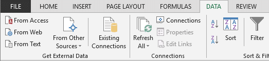
Features under the Get External Data section help create a connection with sources like other workbooks, databases, text files, or websites. Connections section contains features for managing existing connections. To begin creating a new link, click Connections. You will be taken to the Workbook Connections window.

When you connect an external data in Excel, data will be first saved in the workbook. This data can then be exported in other formats, such as Office Data Connection (ODC) (.odc), or a Universal Data Connection (UDC) file (.udcx), to save or share the information.
Creating a data connection
Follow the steps below to connect an external data source to your workbook.
- Begin by going to the Data tab and selecting the connection type that corresponds to your data source. In this example, we are using a Microsoft Access database. Please note that the exact steps will be different if you choose another data type. For example, while you need to select a file for an Access or a text file, you will need to enter the server address for a SQL database. Click the From Access icon to connect to an Access file.

- Select your file and click Open.

- Select Table window will appear. Select the table you’d like to use and click OK to continue.

- In the Import Data window, you can choose how and where to display your data, and you can access advanced settings by pressing the Properties You don’t have to this now as you can open the Properties window at any time after creating connection.


In our example, we choose the Table option. Here is brief summary of all options.
- Table: Data is displayed in a tabular form
- PivotTable Report: You can use the columns to create a PivotTable
- PivotChart: You can use the columns to create a PivotChart
- Only Create Connection: Data will not be displayed, but the connection can be used by other features or VBA, and can be exported.
- Add this data to Data Model: Data is added to the Power Pivot Data Model. This option is independent from the display option above. However, it is advisable to use it with Only Create Connection option, because you can manage your data better in the Data Model.
You can choose to pull certain columns, instead of the entire table, if necessary. Try the PivotTable and Only Create Connection options to create connections without displaying the data in your spreadsheet.
Refreshing and managing data connections
There are several ways to refresh existing connections. The first method is by using the icons under both DATA and TABLE TOOLS — DESIGN tabs in the ribbon. These icons can be used to refresh data connection manually.
Both options essentially do the same thing. However, the default actions are different for the Refresh buttons in the DATA and TABLE TOOLS – DESIGN tabs. While Refresh All action is the default action in DATA tab. Refresh action is the default in the TABLE TOOLS – DESIGN tab. The Refresh button only refreshes the active table’s connection.

Power Pivot and Power Query windows also contain refresh buttons.

To automate this process, you can set a time interval to refresh data connections. To set a refresh interval, and manage the connections (including advanced Properties), use the Connections button to open the Workbook Connections window. You can add new connections, or refresh existing ones in this menu. Select the existing connection and click the Properties button to open Connection Properties window.
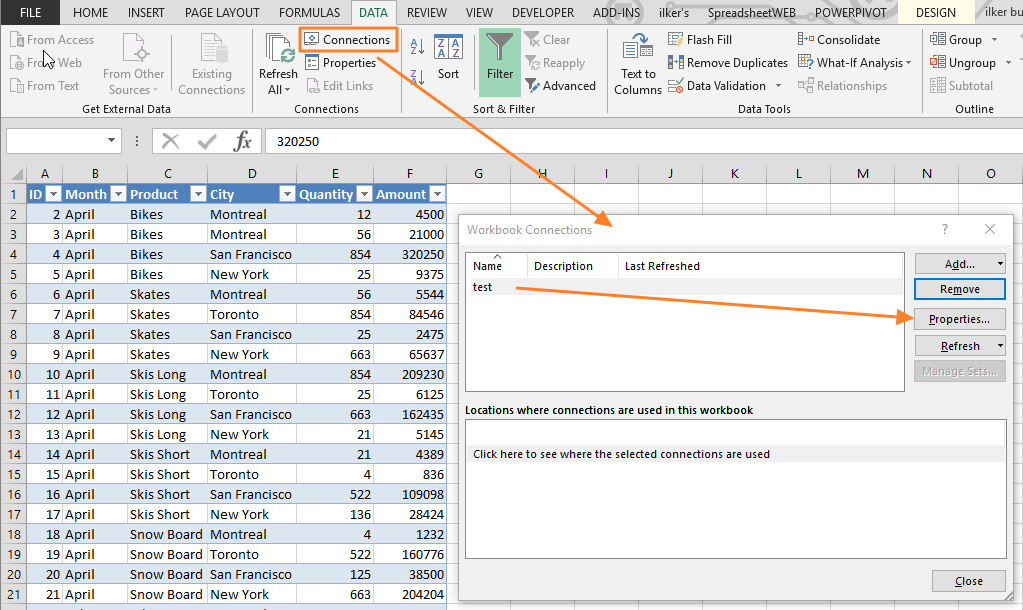
Enable the Refresh every option and modify the number that represents minutes. When you click OK, your data connection will be updated in selected intervals.
An alternative way to automatically refresh data is using VBA. This allows combining data connection features with your own custom code. Below is sample codes that can refresh data connections.
    ActiveWorkbook.Connections("test").Refresh 'Refresh only the connection named "test"

    ActiveWorkbook.RefreshAll 'Refresh all connections