Weighting averages in excel

Usually when you calculate an average, all of the numbers are given equal significance; the numbers are added together, and then, divided by the number of numbers. With a Weighted Average, one or more numbers is given a greater significance, or weight.

Find a Weighted Average

Use the SUMPRODUCT and the SUM functions to find a Weighted Average, which depends on the weight applied to the values.

• For example, a shipment of 10 cases of pencils is 20 cents per case. But a second shipment of 40 cases costs 30 cents per case, because pencils are in high demand. If you averaged the cost of each shipment this way (0.20+0.30)/2 = 0.25, the result isn’t accurate.

  The math doesn’t take into account that there are more cases being sold at 30 cents than at 20 cents. To get the correct average, use this formula to get the result (28 cents per shipment):

  =SUMPRODUCT(A2:A3,B2:B3)/SUM(B2:B3)

  The formula works by dividing the total cost of the two orders by the total number of cases ordered.

Want more?

Calculate the average of a group of numbers

AVERAGE function

AVERAGEIF function

Usually when you calculate an average, all of the numbers are given equal significance.

The numbers are added together and then divided by the number of numbers, as in this example, which returns an unweighted average of 5.

With a Weighted Average, one or more numbers is given a greater significance, or weight.

In this example, the Mid-term and Final exams have a greater weight than Tests 1 and 2.

We’ll use the SUMPRODUCT and SUM functions to determine the Weighted Average.

The SUMPRODUCT function multiplies each Test’s score by its weight, and then, adds these resulting numbers.

We then divide the outcome of SUMPRODUCT by the SUM of the weights.

And this returns the Weighted Average of 80.

SUMPRODUCT is essentially the Sum of Test 1 times its weight, plus the Mid-term times its weight, and so on.

To get the Weighted Average, you divide by the Total of the weights.

If we had just averaged the Test scores, the value would be 75.5, a significant difference.

For more information about the SUMPRODUCT and SUM functions, see the course summary.

Now, you have a good idea about how to average numbers in Excel.

Of course, there’s always more to learn.

So, check out the course summary at the end, and best of all, explore Excel 2013 on your own.

We all know how averages work, right? Means or averages are easily calculable and represent a central value. That’s all fine for regular numbers but the more factors you add, the average value starts seeming a bit misrepresentative.

This can be resolved by associating some quantitative data to each number that will work as weights. Their inclusion in calculating an average gives more weightage to the numbers, slightly shifting the final value from the central value towards the weighted values.

With a bit more demonstration, you will master the weighted average in no time. This tutorial will give you a full picture of weighted averages. What a weighted average really is, how it differs from the average we all know, and how to calculate it. Let’s see what this is all about.

What is Weighted Average?

Weighted average or mean calculates the average of numbers in a dataset by multiplying the numbers to their respective weights. The weights signify the importance or probability of the numbers and therefore, a weighted average delivers a more accurate average. If all the numbers held equal weight or importance, the average of those numbers would equal their weighted average.

A weighted average is calculated by summation of the weights multiplied by the numbers. This value is then divided by the sum of the weights. The syntax for the weighted average is as follows:

Weighted Average = (number1 x weight1) + (number2 x weight2) + ……. / sum of weights

Average vs Weighted Average

An average is the central value in a dataset and is calculated by dividing the sum of the numbers by the number of the numbers. From the formula shown above, we can conclude that there is no weightage involved. Let’s talk about the difference in concept of the two averages without the numbers first.

The most common example of a weighted average, one you may have encountered yourself is that of grading in a semester. Let’s say that students’ performance will be assessed based on their marks on a class test, assignment, mock exam, and final exam.

If a student does exceptionally well in the test and assignment, they wouldn’t need to score well in the exam because the overall total would average out the performance. But if weights were assigned to each, giving more importance to the final exam, the students will take the exam seriously and their overall assessment would be better represented by a weighted average.

Now we can proceed with the numbers.

Let’s get averaging!

Calculate Weighted Average Using SUM Function

Calculating a weighted average does require summation and nothing does summing better than the SUM function. The basic of them all, SUM function adds all the numbers in a range of cells. For calculating a weighted average, the SUM function can help us by adding the product of the numbers and weights for the numerator and for adding the weights in the denominator.

Let’s move on to the formula for calculating the weighted average using the SUM function:

=SUM(C3:C10*D3:D10)/SUM(D3:D10)

Let’s understand the scenario first. Suppose we’re house-hunting. We have a few options and need help deciding so we’ve stacked up a list of factors and scored the houses out of 10 on those factors. For easiness’ sake, instead of writing e.g. 7/10, we’ll write the score as 0.7. We’ve also added weights to those factors according to how much each factor is important to us in a house.

An example of the rating of one house is shown below with the scores in column C and the related weights in column D. Using the SUM function, we have multiplied the scores in C3:C10 by the weights in D3:D10. The outcome will be divided by the sum of the weights in D3:D10 and we arrive at our weighted average score of 0.70.

Now if you look at the average score, which is calculated by applying the AVERAGE function on C3:C10, we can see that this house scores 0.73 or 7.3 out of 10. If we then consider the weights, the factors with lower weightage have pretty high scores and the most important factor, the interior has the least score. Therefore, the weighted average is a truer reflection of the average as it takes into account the importance of each value included in the calculation of the average.

Calculate Weighted Average Using SUMPRODUCT Function

The SUM function was easy to understand and familiar. Weighted averages can also be calculated with the SUMPRODUCT function which also offers a very simple formula. The SUMPRODUCT function returns the sum of the products of corresponding ranges. Let’s have a look at the formula and calculate the weighted average:

=SUMPRODUCT(C3:C10,D3:D10)/SUM(D3:D10)

The formula is very similar to the previous one we used but for multiplying column C with D, we have incorporated the SUMPRODUCT function. SUMPRODUCT multiplies one by one the values in C3:C10 with the corresponding values in D3:D10 (0.7 x 15%, 0.8 x 5%…..).

In the second part of the formula, the sum of the products is divided by the total weights. The total is performed using the SUM function. The final figure we get is the weighted average score of 0.7. This result is consistent with the one of SUM function so we know we’re on the right track.

The weights in this example equal 100%. However, this is not necessary for the calculation, you will still arrive at a weighted average if the weights do not add up to 100%. The formula also doesn’t require the weights in percentages. See another example below to find out how to work with non-percentage weights.

Weights not as Percentages

It’s not important for the weights to be in percentages. Our weights in the next example are quantitative data. Using the SUMPRODUCT function we will calculate the weighted average in an identical manner. This is the formula:

=SUMPRODUCT(C3:C7,D3:D7)/SUM(C3:C7)

In this example case, we have a product i.e. Product 1 of 50 grams made up of 5 materials of varying prices. The quantities of the 5 materials in Product 1 are listed below. To find out on average, the price of each material that goes into the finished product, we’ve calculated a weighted average price.

The SUMPRODUCT function calculates the total of the column C values multiplied by the respective column D values. This amount is denominated by the total of the materials used, mentioned in C3:C7, using the SUM function. The final outcome is the weighted average price of $1.03 which differs from the arithmetic mean of $1.05.

Just a while ago we said we were on the right track and we’ve finished already! See how easy that was? It might sound a little daunting but a weighted average is only a meaningful average, that is all and we have shown you two simple ways of calculating it.

It is our mission to take the trouble out of your Excel troubles and we’re going at it non-stop! See you on the other side of another Excel solution!

When you’re calculating the average for a set of values, you’re generally working with values that have the same weight and importance.

But what happens if some values weigh more than others? This is where the weighted average formula comes in.

In this article, we will break down how to use this formula in Excel, plus provide some examples.

How to Calculate Weighted Average in Excel

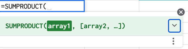
To calculate the weighted average in Excel, you must use the SUMPRODUCT and SUM functions using the following formula:

=SUMPRODUCT(X:X,X:X)/SUM(X:X)

This formula works by multiplying each value by its weight and combining the values. Then, you divide the SUMPRODUCT but the sum of the weights for your weighted average.

Still confused? Let’s go over the steps in the next section.

Using SUMPRODUCT to Calculate Weighted Average in Excel

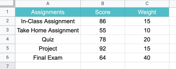
1. Enter your data into a spreadsheet then add a column containing the weight for each data point.

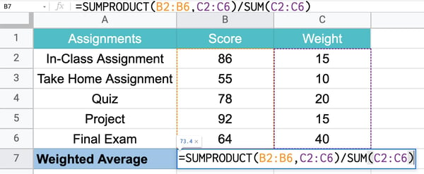
2. Type =SUMPRODUCT to start the formula and enter the values.

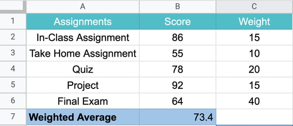
3. Click enter to get your results.

How to Find Weighted Moving Averages in Excel

A weighted moving average is a technique used to keep the time period of the average the same as you add new data or give more weight to certain time periods. This can allow you to identify trends and patterns more easily.

For instance, say you have the number of views your website got in the last five days, you can easily determine the average views in a five-day period.

Now, say the next week, I ask for the five-day average, you would use data from the last five days, not the original five days from the previous week.

As such, you’re still relying on the same time period but updating the data to generate the moving average.

For a weighted moving average, you give more weight to certain time periods than others. You may say that day 5 weights 60% with the remaining percentages decreasing by day.

As such, you’ll need to manually calculate this formula.

WMA = [value 1 x (weight)] + [value 2 x (weight)] + [value 3 x (weight)] + [value 4 x (weight)]

Once you get the hang of it, using the weighted average formula is easy. All it takes is a little practice.

When we calculate a simple average of a given set of values, the assumption is that all the values carry an equal weight or importance.

For example, if you appear for exams and all the exams carry a similar weight, then the average of your total marks would also be the weighted average of your scores.

However, in real life, this is hardly the case.

Some tasks are always more important than the others. Some exams are more important than the others.

And that’s where Weighted Average comes into the picture.

Here is the textbook definition of Weighted Average:

Now let’s see how to calculate the Weighted Average in Excel.

Calculating Weighted Average in Excel

In this tutorial, you’ll learn how to calculate the weighted average in Excel:

• Using the SUMPRODUCT function.
• Using the SUM function.

So let’s get started.

Calculating Weighted Average in Excel – SUMPRODUCT Function

There could be various scenarios where you need to calculate the weighted average. Below are three different situations where you can use the SUMPRODUCT function to calculate weighted average in Excel

Below are three different situations where you can use the SUMPRODUCT function to calculate weighted average in Excel

Example 1 – When the Weights Add Up to 100%

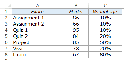
Suppose you have a dataset with marks scored by a student in different exams along with the weights in percentages (as shown below):

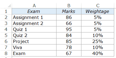
In the above data, a student gets marks in different evaluations, but in the end, needs to be given a final score or grade. A simple average can not be calculated here as the importance of different evaluations vary.

For example, a quiz, with a weight of 10% carries twice the weight as compared with an assignment, but one-fourth the weight as compared with the Exam.

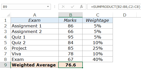
In such a case, you can use the SUMPRODUCT function to get the weighted average of the score.

Here is the formula that will give you the weighted average in Excel:

=SUMPRODUCT(B2:B8,C2:C8)

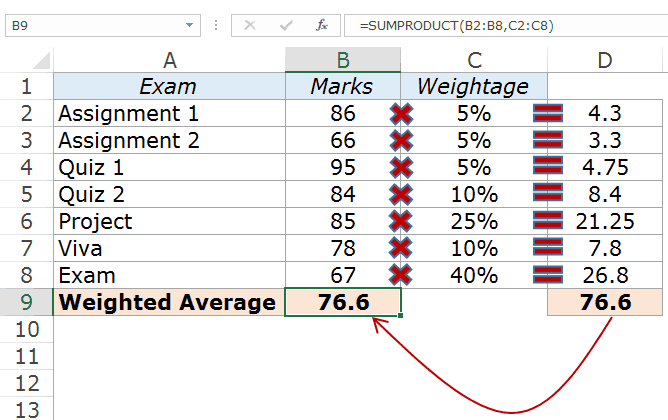
Here is how this formula works: Excel SUMPRODUCT function multiplies the first element of the first array with the first element of the second array. Then it multiplies the second element of the first array with the second element of the second array. And so on..

And finally, it adds all these values.

Here is an illustration to make it clear.

Example 2 – When Weights Don’t Add Up to 100%

In the above case, the weights were assigned in such a way that the total added up to 100%. But in real life scenarios, it may not always be the case.

Let’s have a look at the same example with different weights.

In the above case, the weights add up to 200%.

If I use the same SUMPRODUCT formula, it will give me the wrong result.

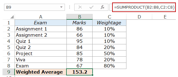
In the above result, I have doubled all the weights, and it returns the weighted average value as 153.2. Now we know a student can’t get more than 100 out of 100, no matter how brilliant he/she is.

The reason for this is that the weights don’t add up to 100%.

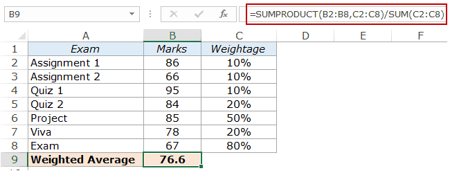
Here is the formula that will get this sorted:

=SUMPRODUCT(B2:B8,C2:C8)/SUM(C2:C8)

In the above formula, the SUMPRODUCT result is divided by the sum of all the weights. Hence, no matter what, the weights would always add up to 100%.

One practical example of different weights is when businesses calculate the weighted average cost of capital. For example, if a company has raised capital using debt, equity, and preferred stock, then these will be serviced at a different cost. The company’s accounting team then calculates the weighted average cost of capital that represents the cost of capital for the entire company.

Example 3 – When the Weights Need to be Calculated

In the example covered so far, the weights were specified. However, there may be cases, where the weights are not directly available, and you need to calculate the weights first and then calculate the weighted average.

Suppose you are selling three different types of products as mentioned below:

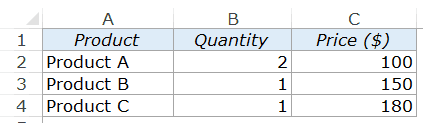
You can calculate the weighted average price per product by using the SUMPRODUCT function. Here is the formula you can use:

=SUMPRODUCT(B2:B4,C2:C4)/SUM(B2:B4)

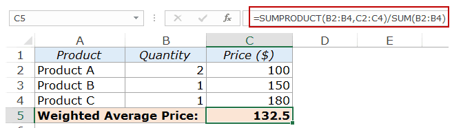
Dividing the SUMPRODUCT result with the SUM of quantities makes sure that the weights (in this case quantities) add up to 100%.

Calculating Weighted Average in Excel – SUM Function

While SUMPRODUCT function is the best way to calculate the weighted average in Excel, you can also use the SUM function.

To calculate the weighted average using the SUM function, you need to multiply each element, with its assigned importance in percentage.

Using the same dataset:

Here the formula that will give you the right result:

=SUM(B2*C2,B3*C3,B4*C4,B5*C5,B6*C6,B7*C7,B8*C8)

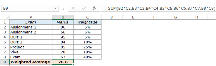
This method is alright to use when you have a couple of items. But when you have many items and weights, this method could be cumbersome and error-prone. There is shorter and better way of doing this using the SUM function.

Continuing with the same data set, here is the short formula that will give you the weighted average using the SUM function:

=SUM(B2:B8*C2:C8)

The trick while using this formula is to use Control + Shift + Enter, instead of just using Enter. Since SUM function can not handle arrays, you need to use Control + Shift + Enter.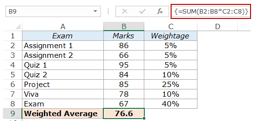

When you hit Control + Shift + Enter, you would see curly brackets appear automatically at the beginning and the end of the formula (see the formula bar in the above image).

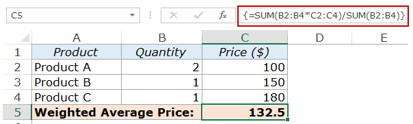
Again, make sure the weights add up to 100%. If it does not, you need to divide the result by the sum of the weights (as shown below, taking the product example):

You May Also Like the Following Excel Tutorials:

• How to Calculate CAGR in Excel
• 5 Easy Ways to Calculate Running Total in Excel (Cumulative Sum)
• Calculating Loan Payment Using PMT Function
• How to Calculate and Format Percentages in Excel
• How to Calculate Age in Excel using Formulas
• Calculating Standard Deviation in Excel
• Calculating Compound Interest in Excel
• Calculating Moving Average in Excel [Simple, Weighted, & Exponential]
• How to Calculate Average Annual Growth Rate (AAGR) in Excel

The weighted average (also known as the weighted mean) is a calculation that provides an average where each value does not carry an equal impact on the final result. Using Excel’s AVERAGE function in these scenarios would give a misleading result. Thankfully, we can easily calculate the weighted average in Excel too.

When to use a weighted average?

It’s not always easy to know when to calculate an average vs. a weighted average. Here are some examples to help you see where a weighted average is the correct calculation.

• In education, all assessments and exams do not have the same impact on the final grade. For example, at university, my final paper counted as 40% of my overall result, with other exams all having equal value. Therefore, we need to calculate the correct result by using a weighted average.
• Looking at average payment terms for suppliers can be a way to understand cash flow. For example, if a business has 10 suppliers with varying payment terms from 7 to 60 days, it may be tempting to use an average. However, if one supplier is 85% of total spend and only that supplier has 7-day terms, then it is necessary to use a weighted average. That one supplier will have a massive impact on the final result.
• A company may calculate its weighted average cost of capital, and use this as the discount rate to assess projects/investments. The idea is that if capital costs 4%, then we need projects to make a return larger than 4%. Otherwise, the cost of financing the project is more than the project returns, so it would be better not to invest at all.

The calculations above clearly demonstrate the importance of selecting the correct calculation. The average calculations would be mathematically accurate; however, they would be the wrong measure for decision-making.

Basic calculation

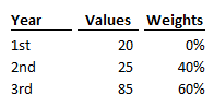
Here is a basic scenario. For a qualification, 40% of Year 2 and 60% of Year 3 count towards the final grade. One student’s results are as follows, what is their final grade?

To calculate a weighted average:

• Step 1: Each value is multiplied by the the corresponding weight
  20 x 0% = 0
  25 x 40% = 10
  85 x 60% = 51
• Step 2: Calculate the sum of each item from Step 1
  0 + 10 + 51 = 61
• Step 3: Divide the result from Step 2 by the SUM of total weights.
  61 / (0% + 40% + 60%) = 61%

The final result is 61%

We can use simple functions to calculate the weighted average in Excel.

Traditional Excel

=SUMPRODUCT(weights,values)/SUM(weights)

Dynamic Array enabled Excel

=SUM(weights*values)/SUM(weights)

To use these formulas, we just need to insert the weights and values for our data. Let’s look at this with the 3 examples we introduced earlier.

Weighted average to calculate exam results

In this scenario, 10 exams and one written paper contribute to the final result. The written paper is worth 40% of the final result; therefore, each exam is only worth 6% of the result.

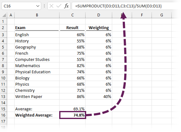
The formula in Cell C16 is:

=SUMPRODUCT(D3:D13,C3:C13)/SUM(D3:D13)

The SUMPRODUCT function achieves Steps 1 and 2 of the calculation; it multiplies each value with each corresponding weight and aggregates the total. Finally, step 3 calculates as the result of SUMPRODUCT divided by the SUM of the weights.

Exam results are a reasonably straightforward scenario to understand. The total weights add to 100%, so we can have a gut feeling about whether the total looks accurate.

Weighted average to calculate average payment terms

In this scenario, we have one supplier on 7-day terms who is 85% of the cost, and then 7 other suppliers varying from 30 to 60 days.

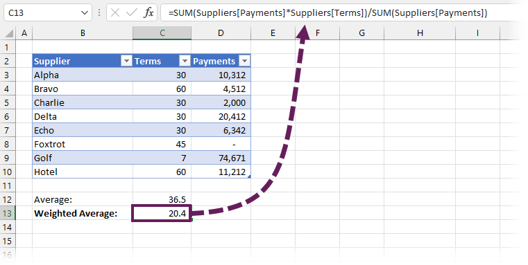
The values have been entered inside an Excel Table, and I am using a dynamic array enabled version of Excel. Therefore, I can use a calculation with only SUM functions.

The formula in Cell C13 is:

=SUM(Suppliers[Payments]*Suppliers[Terms])/SUM(Suppliers[Payments])

The first SUM function achieves Steps 1 and 2 (i.e., the multiplication and initial aggregation). Then in Step 3, the result is divided by the aggregated of the weights.

If we don’t have a dynamic array-enabled version of Excel, we can still use this method. Press Ctrl + Shift + Enter to confirm the formula. This will surround the formula in curly brackets, as shown below, and calculate the correct value in all versions of Excel.

{=SUM(Suppliers[Payments]*Suppliers[Terms])/SUM(Suppliers[Payments])}

Weighted average cost of capital (WACC)

For this final example, we calculate a common business requirement: weighted average cost of capital in Excel.

Weighted average cost of capital (WACC) has the added complexity that the cost of debt is tax-deductible while return on equity is not. In practical terms, it means the published debt rate needs to be adjusted for tax before being included in the calculation.

The numbers below are based on an article from investopedia.com. The company’s equity of $394B has a cost of 4.99%, while the debt of $44B has a cost of 3.99%. The debt rate is adjusted for a 33% tax rate.

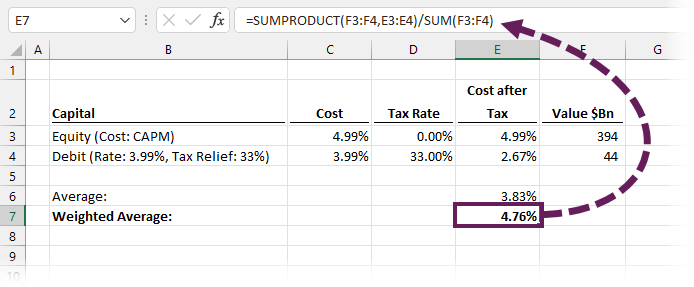
The formula in Cell E7 is:

=SUMPRODUCT(F3:F4,E3:E4)/SUM(F3:F4)

This example demonstrates that in some scenarios, we may need to adjust values where there are factors affecting some numbers but not others. We want to calculate on a consistent basis.

Common errors

Here are some common errors you might encounter when calculating weighted average in Excel:

• In the multiplication, the #VALUE! error will be returned if the ranges or arrays are of different sizes. This is true for the SUMPRODUCT or SUM approach.
• SUMPRODUCT and SUM both treat text as zeros, so if your ranges contain any text, it may not calculate the correct result

Conclusion

There is no weighted average function in Excel, but with two simple functions, SUMPRODUCT and SUM, we can easily calculate it ourselves.