
Excel for Microsoft 365 Excel for Microsoft 365 for Mac Excel for the web Excel 2021 Excel 2021 for Mac Excel 2019 Excel 2019 for Mac Excel 2016 Excel 2016 for Mac Excel 2013 Excel 2010 Excel 2007 Excel for Mac 2011 Excel Starter 2010 More…Less
This article describes the formula syntax and usage of the WEEKDAY
function in Microsoft Excel.
Description
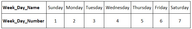
Returns the day of the week corresponding to a date. The day is given as an integer, ranging from 1 (Sunday) to 7 (Saturday), by default.
Syntax
WEEKDAY(serial_number,[return_type])
The WEEKDAY function syntax has the following arguments:
-
Serial_number Required. A sequential number that represents the date of the day you are trying to find. Dates should be entered by using the DATE function, or as results of other formulas or functions. For example, use DATE(2008,5,23) for the 23rd day of May, 2008. Problems can occur if dates are entered as text.
-
Return_type Optional. A number that determines the type of return value.
|
Return_type |
Number returned |
|
1 or omitted |
Numbers 1 (Sunday) through 7 (Saturday). Behaves like previous versions of Microsoft Excel. |
|
2 |
Numbers 1 (Monday) through 7 (Sunday). |
|
3 |
Numbers 0 (Monday) through 6 (Sunday). |
|
11 |
Numbers 1 (Monday) through 7 (Sunday). |
|
12 |
Numbers 1 (Tuesday) through 7 (Monday). |
|
13 |
Numbers 1 (Wednesday) through 7 (Tuesday). |
|
14 |
Numbers 1 (Thursday) through 7 (Wednesday). |
|
15 |
Numbers 1 (Friday) through 7 (Thursday). |
|
16 |
Numbers 1 (Saturday) through 7 (Friday). |
|
17 |
Numbers 1 (Sunday) through 7 (Saturday). |
Remark
-
Microsoft Excel stores dates as sequential serial numbers so they can be used in calculations. By default, January 1, 1900 is serial number 1, and January 1, 2008 is serial number 39448 because it is 39,448 days after January 1, 1900.
-
If serial_number is out of range for the current date base value, a #NUM! error is returned.
-
If return_type is out of the range specified in the table above, a #NUM! error is returned.
Example
Copy the example data in the following table, and paste it in cell A1 of a new Excel worksheet. For formulas to show results, select them, press F2, and then press Enter. If you need to, you can adjust the column widths to see all the data.
|
Data |
||
|
2/14/2008 |
||
|
Formula |
Description (Result) |
Result |
|
=WEEKDAY(A2) |
Day of the week, with numbers 1 (Sunday) through 7 (Saturday) (5) |
5 |
|
=WEEKDAY(A2, 2) |
Day of the week, with numbers 1 (Monday) through 7 (Sunday) (4) |
4 |
|
=WEEKDAY(A2, 3) |
Day of the week, with numbers 0 (Monday) through 6 (Sunday) (3) |
3 |
Need more help?
Purpose
Get the day of the week as a number
Return value
A number between 0 and 7.
Usage notes
The WEEKDAY function takes a date and returns a number between 1-7 representing the day of the week. The WEEKDAY function takes two arguments: serial_number and return_type. Serial_number should be a valid Excel date in serial number format. Return_type is an optional numeric code that controls which day of the week is considered the first day. By default, WEEKDAY returns 1 for Sunday and 7 for Saturday, as seen in the table below:
| Result | Meaning |
|---|---|
| 1 | Sunday |
| 2 | Monday |
| 3 | Tuesday |
| 4 | Wednesday |
| 5 | Thursday |
| 6 | Friday |
| 7 | Saturday |
WEEKDAY supports several numbering schemes, controlled by the return_type argument. Return_type is optional and defaults to 1. The table below shows available return_type codes, the numeric result of each code, and which day is the first day in the mapping scheme.
| Return type | Numeric result | Day mapping |
|---|---|---|
| none | 1-7 | Sunday-Saturday |
| 1 | 1-7 | Sunday-Saturday |
| 2 | 1-7 | Monday-Sunday |
| 3 | 0-6 | Monday-Sunday |
| 11 | 1-7 | Monday-Sunday |
| 12 | 1-7 | Tuesday-Monday |
| 13 | 1-7 | Wednesday-Tuesday |
| 14 | 1-7 | Thursday-Wednesday |
| 15 | 1-7 | Friday-Thursday |
| 16 | 1-7 | Saturday-Friday |
| 17 | 1-7 | Sunday-Saturday |
Note: the WEEKDAY function will return a value even when the date is empty. Take care to trap this result if blank dates are possible.
Examples
By default and without a value fore return_type, WEEKDAY starts counting on Sunday:
=WEEKDAY("3-Jan-21") // Sunday, returns 1
=WEEKDAY("4-Jan-21") // Monday, returns 2
To configure WEEKDAY to start on Monday, set return_type to 2:
=WEEKDAY("3-Jan-21",2) // Sunday, returns 7
=WEEKDAY("4-Jan-21",2) // Monday, returns 1
In the example shown above, the formula in D5 (copied down) is:
=WEEKDAY(B5) // Sunday start
The formula in E5 (copied down) is:
=WEEKDAY(B5,2) // Monday start
Notes
- By default, WEEKDAY returns 1 for Sunday and 7 for Saturday.
- WEEKDAY returns a value (7) even if the date is empty.
The WEEKDAY function in excel returns the day corresponding to a specified date. The date is supplied as an argument to this function. The returned day is an integer, which can take any value from 0 to 7. This value is calculated from a beginning day specified by the user.
For example, if the date supplied is August 4, 2018, the WEEKDAY function returns 7 as the output. In this case, the number 7 corresponds to Saturday.

The purpose of using the WEEKDAY() in excel is to ascertain the day coinciding with the given date. This helps calculate the duration of a project, schedule a to-do list, estimate the per-day cost of a service provider, create daily or weekly reports, and so on.
The WEEKDAY function is categorized as a Date and Time function of Excel.
Table of contents
- What is Weekday () Function in Excel?
- Syntax of the WEEKDAY Function of Excel
- Outputs of the WEEKDAY Function When the “Return_Types” Differ
- How to Use the WEEKDAY Function in Excel?
- Example #1–Use the WEEKDAY Function to Compare Outputs Having Different “Return_Types”
- Example #2–Use the Nested IF, CHOOSE and WEEKDAY, and TEXT Functions to Extract the Name of Days
- Example #3–Use the IF, OR, and WEEKDAY Functions to Separate Weekdays from Weekends
- Example #4–Use the IF, WEEKDAY, and SUM Functions to Calculate the Per-Day Cost of a Service Provider
- Frequently Asked Questions
- WEEKDAY Excel Function Video
- Recommended Articles
Syntax of the WEEKDAY Function of Excel
The syntax of the WEEKDAY excel function is shown in the following image:
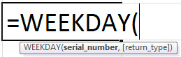
The WEEKDAY() in excel accepts the following arguments:
- Serial_number: This is the date for which the respective day is required. It can be entered as a direct date, sequential number representing a date or a cell reference containing a date.
- Return_type: This decides from which day the calculation of the output should begin. It can take any value from 1-3 and 11-17. For instance, if this argument is entered as 1, the week starts from Sunday (beginning day counted as 1) and ends on Saturday (ending day counted as 7). In this case, the output 2 represents Monday, 3 stands for Tuesday, and so on.
The “serial_number” is a required argument, while “return_type” is an optional one. When the “return_type” argument is omitted, Excel assumes it as 1.
Note: Excel stores dates as sequential numbers called serial values or serial numbers. The first date is January 1, 1900, which is stored as number 1. The last date is December 31, 9999, which is stored as the number 2958465.
Outputs of the WEEKDAY Function When the “Return_Types” Differ
The outputs obtained by the different values of the “return_type” argument are listed as follows:
When the “return_type”=1, the outputs 1 and 7 signify Sunday and Saturday respectively. So, the week starts from Sunday and ends on Saturday.

When the “return_type”=2, the outputs 1 and 7 signify Monday and Sunday respectively. So, the week starts from Monday and ends on Sunday.
When the “return_type”=3, the outputs 0 and 6 signify Monday and Sunday respectively. So, the week starts from Monday and ends on Sunday.

When the “return_type” ranges from 11 to 17, the outputs obtained are listed as follows:

Note 1: The “return_type” values ranging from 11 to 17 were introduced in Excel 2010. So, in the earlier versions of Excel, only values 1 to 3 of the “return_type” argument are available. However, the WEEKDAY function is available in all versions of Excel.
Note 2: If the “return_type” argument is supplied (to the WEEKDAY function) as a value other than 1 to 3 or 11 to 17, Excel returns the “#NUM!” error.
How to Use the WEEKDAY Function in Excel?
Let us consider some examples to understand the working of the WEEKDAY() in excel .
You can download this WEEKDAY Function Excel Template here – WEEKDAY Function Excel Template
Example #1–Use the WEEKDAY Function to Compare Outputs Having Different “Return_Types”
The succeeding image shows some dates (in column A), which pertain to August 2018. We want to perform the following tasks:
- Supply each date to the WEEKDAY function to obtain the corresponding days.
- Observe the different outputs when the “return_type” argument is set at 1, 2, and 3. Set one “return_type” in one column.
The steps to perform the given tasks are listed as follows:
Step 1: Supply the cell reference of each date to the WEEKDAY function. For this, enter the following WEEKDAY formulas in row 2 of three different columns.
- “=WEEKDAY(A2,1)”
- “=WEEKDAY(A2,2)”
- “=WEEKDAY(A2,3)”
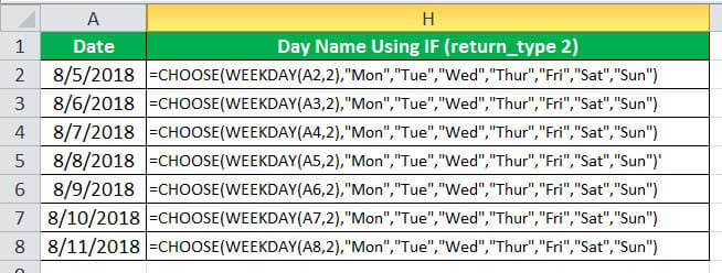
We have set the “return_type” argument as 1, 2, and 3 in the different columns. For ease of understanding, we have given the different formulas in the following image.

Step 2: Press the “Enter” key after entering each formula of row 2. Drag the formula of row 2 till row 8 of the three columns.
The outputs are shown in the following image. We have retained the dates in column A and displayed the outputs in columns B, D, and F.
The “return_type” argument is set at 1, 2, and 3 for columns B, D, and F respectively.

Step 3: The consolidated results are shown in the following image.
Note: This step has been added only to facilitate comparisons across the changing “return_type” arguments. However, steps 1 and 2 are complete within themselves.

Explanation: When “return_type” is 1, the date 5th August is a Sunday, 6th August is a Monday, and 7th August is a Tuesday. This is because the week starts from Sunday (output 1) and ends on Saturday (output 7).
Similarly, when “return_type” is 2 and 3, the date 5th August still falls on Sunday, 6th August is a Monday, and so on. This is because, with “return_type”=2, the week starts from Monday (output 1) and ends on Sunday (output 7).
Likewise, for “return_type”=3, the week starts from Monday (output 0) and ends on Sunday (output 6).
Hence, Excel returns the correct day irrespective of the “return_type” specified in the WEEKDAY function. With the different “return_types,” each day is counted differently, though the final interpretation stays the same.
Example #2–Use the Nested IF, CHOOSE and WEEKDAY, and TEXT Functions to Extract the Name of Days
Working on the dataset of example #1, we want to replace each numeric output (of example #1) with the corresponding day of the week. For instance, in place of 1, the output should be Sunday. The “return_type” values and the functions of Excel to be used are stated as follows:
- For “return_type” values 1, 2, and 3: The IF and WEEKDAY excel functions should return the full names of the different days as the output.
- For “return_type” values 1 and 2: The CHOOSE and W should return the first three letters of the different days as the output.
- For “return_type” value 3: The TEXT function should return the full names of the different days as the output.
Work on each “return_type” value one by one. Create three cases with the “return_type” argument as 1, 2, and 3.
Case 1: The “return_type” argument is 1.
a. The steps to use the IF and WEEKDAY excel functions for the given task are listed as follows:
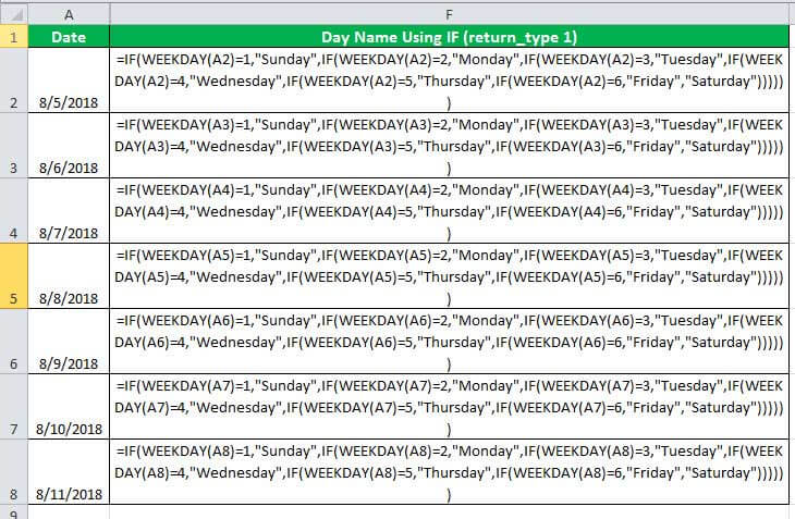
Step 1: Enter the following formula in cell F2.
IF(WEEKDAY(A2)=4,”Wednesday”,IF(WEEKDAY(A2)=5,”Thursday”,
IF(WEEKDAY(A2)=6,”Friday”,”Saturday”))))))
For ease of understanding, the IF and WEEKDAY formulas for the entire range (F2:F8) are shown in the following image. Since the “return_type” argument is 1 for all WEEKDAY formulas, we have omitted it.
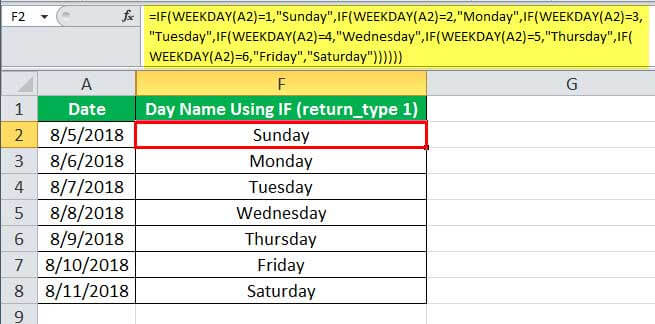
Step 2: Press the “Enter” key once the complete formula has been entered in cell F2. Drag the formula of cell F2 till cell F8. The outputs of column F are shown in the following image.
Hence, the full names of the different days have been obtained with the help of the IF and WEEKDAY functions.
Explanation: The formula entered in step 1 (of this example) is a nested IF formula. With this formula, Excel is given the following instructions:
- If the logical test “WEEKDAY(A2)=1” is true, return the string “Sunday.” If this logical test is false, evaluate the second logical test.
- Next, if the logical test “WEEKDAY(A2)=2” is true, return the string “Monday.” If this logical test is false, evaluate the next logical test. This evaluation of logical tests goes on till the last logical test.
- Thereafter, if the last logical test “WEEKDAY(A2)=6” is true, return the string “Friday.” If this logical test is false, return the string “Saturday.” The string “Saturday” is returned when none of the supplied logical tests is true.
Hence, Excel evaluates all the given logical tests, which are represented by the different WEEKDAY formulas. Accordingly, an output is returned depending on whether a particular logical test is met or not.
Note: The syntax of the IF function is “IF(logical_test,[value_if_true],[value_if_false]).” The “logical_test” is the condition to be evaluated. The “value_if_true” is returned if the “logical_test” evaluates to true. The “value_if_false” is returned if the “logical_test” evaluates to false.
b. The steps to use the CHOOSE and WEEKDAY excel functions for the mentioned task are listed as follows:
Step 1: Enter the following formula in cell F2.
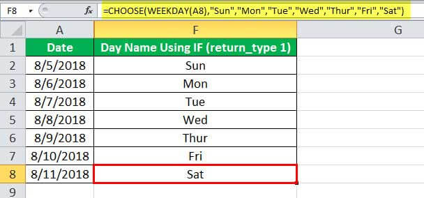
“=CHOOSE(WEEKDAY(A2),”Sun”,”Mon”,”Tue”,”Wed”,”Thur”,”Fri”,”Sat”)”
To help the reader understand, the formulas for the entire range (F2:F8) are shown in the following image. Notice that the “return_type” argument has been omitted in all these formulas.
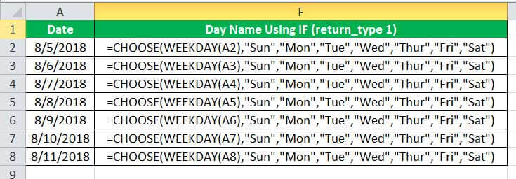
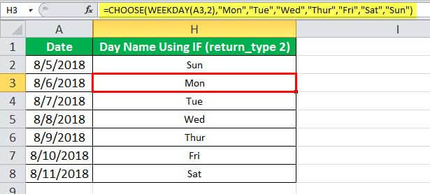
Step 2: Press the “Enter” key once the formula has been entered in cell F2. Drag this formula till cell F8. The outputs of column F are shown in the following image.
Hence, the first three letters of the different days have been obtained by using the CHOOSE and WEEKDAY functions.
Explanation: The formula “WEEKDAY(A2)” entered as a part of the CHOOSE formula (in step 1) returns the number 1. This output of the WEEKDAY function is considered as the “index_num” argument of the CHOOSE function.
Since the “index_num” argument is 1 (for cell F2), the CHOOSE function returns the first value (Sun) from the given list of values (“Sun,” “Mon,” Tue,” etc.). Likewise, the formula “WEEKDAY(A3)” returns the number 2. So, the “index_num” argument for cell F3 is 2. Consequently, the CHOOSE function returns the second value from the list, which is “Mon.”
Notice that in the given CHOOSE formula, we have entered the values beginning from “Sun” and ending on “Sat.” This is because when the “return_type” argument is set at 1, the week begins on Sunday and ends on Saturday.
Note 1: The syntax of the CHOOSE function is “CHOOSE(index_num,value1,[value2],…).” The “index_num” is the position from which a value is returned. “Value1,” “value2,” “value3,” and so on are the list of values from which a value is returned by the CHOOSE function.
Note 2: If the list of values had consisted of two letters like “Su,” “Mo,” “Tu,” “We” etc., the output also would have contained exactly two letters of each day.
Case 2: The “return_type” argument is 2.
a. The steps to perform the given task with the IF and WEEKDAY functions are listed as follows:
Step 1: Enter the following formula in cell H2.
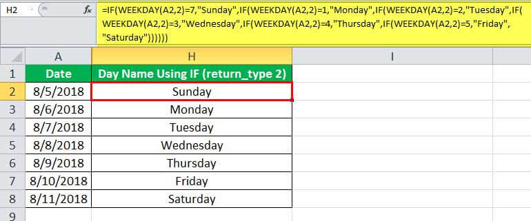
=IF(WEEKDAY(A2,2)=7,”Sunday”,IF(WEEKDAY(A2,2)=1,”Monday”, IF(WEEKDAY(A2,2)=2,“Tuesday”,IF(WEEKDAY(A2,2)=3,”Wednesday”, IF(WEEKDAY(A2,2)=4,”Thursday”,IF(WEEKDAY(A2,2)=5,”Friday”,“Saturday”))))))
For ease of understanding, the IF and WEEKDAY formulas for the range H2:H8 are shown in the following image.
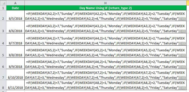
Step 2: Press the “Enter” key once the formula in cell H2 has been entered. Drag this formula till cell H8. The outputs are shown in column H of the following image.
Hence, the complete names of the different days have been obtained by the IF and WEEKDAY functions.
Explanation: Notice that the IF and WEEKDAY formula entered this time is different from the one entered in step 1 of case 1 (pointer “a”). The difference is that the “return_type” argument has been entered as 2 this time. Moreover, the outputs 1 to 7 have been allotted different text strings this time.
For instance, the output 1 (of the WEEKDAY function) has been assigned “Monday” while the output 7 has been allotted the string “Sunday.” In contrast, the output 1 was allotted “Sunday” and 7 was allotted “Saturday” in step 1 of case 1 (pointer “a”).
This change in the allotment of text strings is because the beginning and ending days differ with a change in the “return_type” argument. However, the outputs in step 2 of this case and step 2 of the preceding case (pointer “a”) are the same.
Note: For more details related to the working of the IF and WEEKDAY formula, refer to the “explanation” given after step 2 of case 1 (pointer “a”).
b. The steps to perform the given task with the CHOOSE and WEEKDAY excel functions are listed as follows:
Step 1: Enter the following formula in cell H2.
“=CHOOSE(WEEKDAY(A2,2),”Mon”,”Tue”,”Wed”,”Thur”,”Fri”,”Sat”,”Sun”)”
To help the reader understand, we have given the formulas for the range H2:H8 in the following image.
Step 2: Press the “Enter” key after entering the formula in cell H2. Drag this formula till cell H8. The outputs are shown in the following image.
Hence, the CHOOSE and WEEKDAY functions have returned the first three letters of the different days.
Explanation: Notice that the list of values of the CHOOSE formula (entered in step 1) begins from “Mon” and ends on “Sun.” In contrast, this list began from “Sun” and ended on “Sat” in the CHOOSE formula entered in step 1 of case 1 (pointer “b”).
However, the results of both CHOOSE formulas are the same. In these formulas, the start and end points of the list of values are different. This is because the beginning and ending days vary with a change in the “return_type” argument.
Note: For details related to the syntax and working of the CHOOSE formula, refer to the “explanation” given after step 2 of case 1 (pointer “b”).
Case 3: The “return_type” argument is 3.
a. The steps to perform the given task with the IF and WEEKDAY functions are listed as follows:
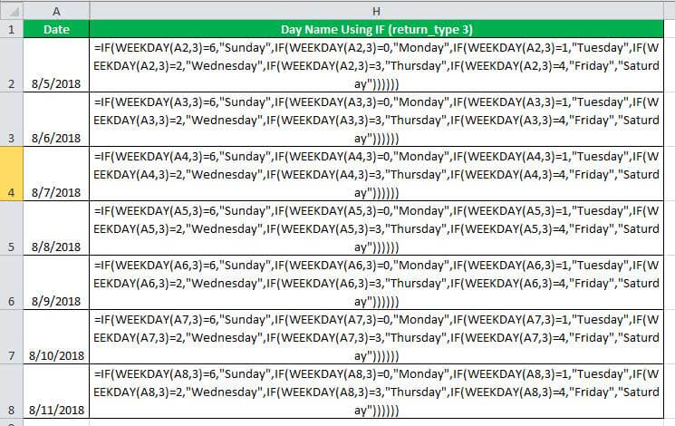
Step 1: Enter the following formula in cell H2.
IF(WEEKDAY(A2,3)=1,”Tuesday”,IF(WEEKDAY(A2,3)=2,”Wednesday”,IF(WEEKDAY(A2,3)=3,”Thursday”,IF(WEEKDAY(A2,3)=4,”Friday”,”Saturday”))))))
For ease of understanding, we have given the IF and WEEKDAY formulas for the entire range in the following image.
Step 2: Press the “Enter” key after the formula in cell H2 has been entered. Next, drag the formula till cell H8. The outputs appear, as shown in the following image.

Explanation: For details related to the working of the IF and WEEKDAY formulas, refer to the “explanation” of pointer “a” of cases 1 and 2. This section is given after step 2 in the preceding cases.
b. The question of this example does not suggest performing the task in pointer “b” when the “return_type” argument is 3.
It must be noticed that for “return_type” value 3, we cannot use the combination of CHOOSE and WEEKDAY functions of Excel. This is because the formula “=WEEKDAY(A3,3)” returns the output 0. If the “index_num” argument of the CHOOSE function is less than 1, it returns the “#VALUE!” error.
c. The steps to perform the given task using the TEXT function are listed as follows:
Step 1: Enter the following formula in cell H2.
“=TEXT(A2,”dddd”)”
To help the reader understand, we have displayed the formulas for the range H2:H8 in the following image.

Step 2: Press the “Enter” key once the formula in step 1 has been entered. Drag this formula till cell H8. The outputs are shown in the following image.
Hence, the full names of the different days have been obtained with the help of the TEXT function.

Explanation: The TEXT formula entered in step 1 has converted the dates (of column A) to text strings (in column H). This conversion has been carried out in the format “dddd.” This format (dddd) represents the complete name of the day.
Note: The syntax of the TEXT function is “TEXT(value,format_text).” The “value” is the numeric value that needs to be converted to a text string. The “format_text” is the format to be applied to the numeric value.
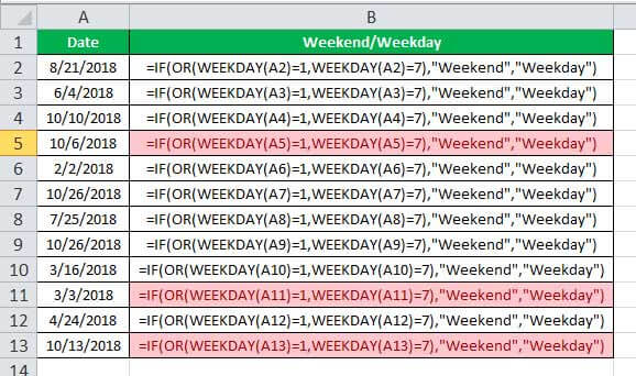
Example #3–Use the IF, OR, and WEEKDAY Functions to Separate Weekdays from Weekends
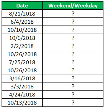
The following image shows some random dates of 2018 in column A. We want to perform the following tasks:
- Determine the weekdays and the weekends (Saturday and Sunday) from the given dates.
- Separate the weekdays from the weekends by coloring the latter pink.
Use the IF, OR, and WEEKDAY functions of Excel. Set the “return_type” argument of the WEEKDAY function as 1.
The steps to perform the given tasks are listed as follows:
Step 1: First, let us recall the outputs returned by the WEEKDAY() in excel when the “return_type” argument is set at 1. In this case, 1 signifies Sunday and 7 implies Saturday. This is shown in the following image.
Step 2: Enter the following formula in cell B2.
“=IF(OR(WEEKDAY(A2)=1,WEEKDAY(A2)=7),”Weekend”,”Weekday”)”
Since the “return_type” argument has been omitted in this formula, Excel considers it as 1. Further, this formula checks whether each cell of column A evaluates to Saturday (output 7) or Sunday (output 1) or to a day other than these two.
If a cell does evaluate to either Saturday or Sunday, the output is “weekend,” otherwise the output is “weekday.”
The following image shows the list of formulas of the range B2:B13. This is given only to make the reader aware of the different formulas used. At this stage, ignore the pink color applied to certain cells.
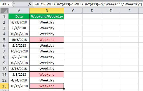
Step 3: Press the “Enter” key after entering the formula in cell B2. Drag this formula till cell B13. The outputs are shown in the following image.
Hence, all dates of column A have been classified as “weekday” or “weekend” in column B. Further, the cells containing “weekend” have been colored pink to distinguish them from the cells containing “weekday.”
Explanation: The formula entered in step 2 (of this example) works as follows:
- The two OR conditions are evaluated first. The first OR condition is “WEEKDAY(A2)=1” and the second OR condition is “WEEKDAY(A2)=7.”
- In the first OR condition, the formula “WEEKDAY(A2)” returns 3, which is not equal to 1. So, this condition evaluates to false.
- In the second OR condition, output 3 of “WEEKDAY(A2)” is compared with 7. Since 3 is not equal to 7, this condition also evaluates to false. For row 2, the final output of both the OR conditions is “false.”
- Next, Excel processes the IF formula. Since the OR conditions have evaluated to false (for row 2), the IF function realizes that the logical test has not been met. So, for row 2, the IF function returns the “value_if_false,” which is “weekday.”
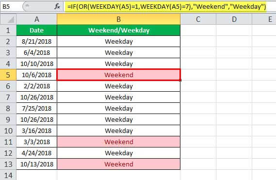
Likewise, all IF formulas of column B work this way. The formula of row 5 has been highlighted in the formula bar of the following image.
In row 5, the first OR condition evaluates to false, while the second OR condition evaluates to true. This is because the formula “WEEKDAY(A5)” returns 7.
Since the final OR output is “true” (for row 5), the IF function realizes that the logical test has been met. Hence, for row 5, the IF function returns the “value_if_true,” which is “weekend.”
Note: The OR function returns “true” if any or all conditions are true. It returns “false” if all conditions are false. For the syntax of the IF function, refer to the “explanation” of case 1 (pointer “a”).
In this way, we can obtain customized responses (like “weekend” and “weekday” in this example) for the other days of the week as well.
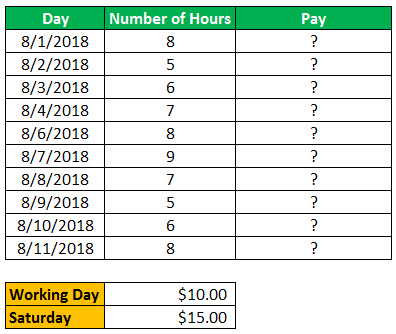
Example #4–Use the IF, WEEKDAY, and SUM Functions to Calculate the Per-Day Cost of a Service Provider
A freelancer provides service to an organization from Monday to Saturday. Each day he works for a few hours and charges as per the following rates:
- $10 per hour for Monday to Friday
- $15 per hour for Saturday
The following image shows the number of hours worked by the freelancer in August 2018. Calculate the total amount paid to the freelancer in the given time period.
Use the IF, WEEKDAY, and SUM functions of Excel. For the WEEKDAY function, set the “return_type” argument as 1.
The steps to calculate the total payment by using the IF, WEEKDAY, and SUM functions are listed as follows:
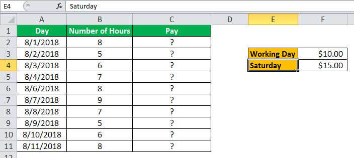
Step 1: First, let us place the boxes containing “working day,” “Saturday,” and their respective amounts in the range E3:F4. These boxes should be next to the dataset since they will be used in the formula of the subsequent step.
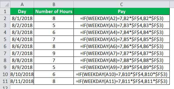
Step 2: Enter the following formula in cell C2.
“=IF(WEEKDAY(A2)=7,B2*$F$4,B2*$F$3)”
The “return_type” argument for the WEEKDAY function has been omitted, implying that Excel will consider it as 1.
For clarity, the IF and WEEKDAY formulas for the range C2:C11 are shown in the following image. Notice that both relative and absolute references have been used in all the formulas.
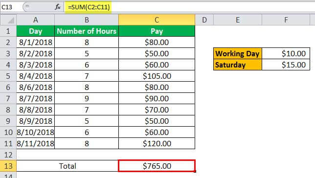
Step 3: Press the “Enter” key once the formula in cell C2 has been entered. Drag this formula till cell C11. The outputs are shown in the following image. The amounts paid for each working day have been obtained.
The highest amount paid is $120 for 11th August 2018, which is a Saturday.

Step 4: Enter the following formula in cell C13. This adds the individual amounts paid.
“=SUM(C2:C11)”
Press the “Enter” key. The output is shown in the following image. Hence, $765 is paid to the freelancer for his service provided in August 2018.
Explanation: The IF and WEEKDAY formula, entered in step 2, gives the following instructions to Excel:
- If the condition “WEEKDAY(A2)=7” is true, multiply the value of cell B2 by the value of cell F4. In other words, if the output of this condition is 7, multiply 5 by 15.
- If the condition “WEEKDAY(A2)=7” is false, multiply the value of cell B2 by the value of cell F3. In other words, if the output of this condition is not 7, multiply 5 by 10.
When the WEEKDAY function returns 7, it corresponds to Saturday. In this case, the number of hours must be multiplied by the rate of Saturday ($15) to find the amount paid for this day.
Likewise, when the output of the WEEKDAY() is not 7, it corresponds to a day other than Saturday. The number of hours is then multiplied by the rate of the other working days ($10). In this way, all outputs of column C have been calculated by the IF and WEEKDAY functions.
Finally, the amounts of column C have been added by using the SUM function. This returns the total amount paid to the freelancer for the given time period.
Frequently Asked Questions
1. Define the WEEKDAY function in Excel with the help of an example.
The WEEKDAY function in Excel returns an integer that represents the day of a specified date. The output returned can take any value from 0 to 7. The day from which this value is calculated can be specified by the user.
For instance, the formula [=WEEKDAY(“14/1/2022”)] returns 6 when entered without the beginning and ending square brackets in Excel. The number 6 represents Friday. In this case, the output has been calculated from 1, which represents Sunday.
Note: For the syntax of the WEEKDAY function, refer to the heading “syntax of the WEEKDAY function of Excel” given in this article.
2. By using the WEEKDAY function of Excel, how can one obtain the names of the days from a date range?
The WEEKDAY function of Excel does not directly return the names of the days. Instead, it returns numerical values by processing each date. These values can then be converted to the names of the days. The steps for the entire process are listed as follows:
a. Enter the WEEKDAY formula adjacent to the cell containing the date. For instance, if the date is in cell A2, the formula in cell B2 should be “=WEEKDAY(A2).” One can set the “return_type” argument as required. Exclude the beginning and ending double quotation marks while entering this formula.
b. Press the “Enter” key once the formula has been entered. If required, drag this formula to the remaining range of cells. The outputs of the WEEKDAY function for the entire range are obtained.
c. Select the range of outputs obtained in the preceding step. Right-click the selection and choose “format cells” from the context menu.
d. The “format cells” window opens. Under “category,” select “custom.” In the box under “type,” enter the format “dddd.” Click “Ok.”
The names of the days are obtained for the entire range of outputs selected in step “c.”
Note: Alternatively, the names of the days can be obtained by using either the TEXT or a mix of CHOOSE and WEEKDAY functions of Excel. For the usage of the TEXT function, refer to the third case of example #2 (pointer “c”).
For the CHOOSE and WEEKDAY formula of Excel, refer to pointer “b” of the first and second cases (example #2). Note that the CHOOSE function cannot be used when the “return_type” argument is 3. This is because the “index_num” argument cannot be zero.
3. With the help of the WEEKDAY function of Excel, how can one check whether a date represents a weekday or weekend?
To check whether a date represents a weekday or weekend, the WEEKDAY formula should be used with the conditional formatting feature of Excel. With this feature, one can highlight the dates representing weekends. This helps distinguish between weekdays and weekends.
The steps to apply conditional formatting with the WEEKDAY formula are listed as follows:
a. Select the date range which needs to be checked for weekdays or weekends.
b. From the Home tab, click the “conditional formatting” drop-down from the “styles” group. Select “new rule.”
c. The “new formatting rule” window opens. Under “select a rule type,” choose the option “use a formula to determine which cells to format.”
d. Under “format values where this formula is true,” enter the OR and WEEKDAY formula. For instance, the range A2:A12 contains dates and the “return_type” argument is 1. Type the formula “=OR(WEEKDAY(A2)=1,WEEKDAY(A2)=7)” without the beginning and ending double quotation marks.
e. Click “format” and choose the desired color from the “fill” tab. Next, click “Ok.”
f. Click “Ok” again in the “new formatting rule” window.
The dates representing weekends (Saturday and Sunday) have been colored in the selected range (selected in step “a”). The dates representing weekdays have not been colored. So, one can easily figure out whether a date represents a weekday or a weekend.
Note 1: Since the “return_type” argument is set at 1, Excel considers Saturday and Sunday as weekends.
Note 2: For “return_type”=2, use the formula “=OR(WEEKDAY(A2,2)=1,WEEKDAY(A2,2)=7)” without the beginning and ending double quotation marks.
So, had the “return_type” argument been set at 2, the two OR conditions would have again been tested for values 1 and 7. However, this time the weekends would have been Monday and Sunday. So, the dates representing these two days would have been highlighted.
WEEKDAY Excel Function Video
Recommended Articles
This has been a guide to the WEEKDAY in Excel. Here we discuss the WEEKDAY formula in Excel and how to use the WEEKDAY function along with Excel examples and downloadable Excel templates. You may also look at these useful functions of Excel–
- WORKDAY in ExcelThe WORKDAY function returns the forthcoming work day after a given number of days from the start date. It has an optional argument for holidays that, if not provided, automatically considers weekends (Saturdays and Sundays) to be holidays.read more
- DAY In ExcelIn Excel, the DAY function calculates the day value from a given date. This function accepts a date as an argument and returns a two-digit numeric value as an integer value representing the given date’s day. The formula to use this function is =Edate(serial number).read more
- TODAY’s Date in ExcelToday function is a date and time function that is used to find out the current system date and time in excel. This function does not take any arguments and auto-updates anytime the worksheet is reopened. This function just reflects the current system date, not the time.read more
- TIME in Excel
- Sentence Case in ExcelThe sentence case excel changes the «case» of the supplied text string. The text string is modified using three functions: UPPER, LOWER, and PROPER. These functions exist because MS Excel lacks a button for changing the case of text.read more
На чтение 2 мин
Функция WEEKDAY (ДЕНЬНЕД) в Excel используется для вычисления порядкового номера дня недели (от 1 до 7).
Содержание
- Что возвращает функция
- Синтаксис
- Аргументы функции
- Дополнительная информация
- Примеры использования функции WEEKDAY (ДЕНЬНЕД) в Excel
Что возвращает функция
Число от «1» до «7» в зависимости от даты, из которой требуется провести расчет.
 Больше лайфхаков в нашем Telegram Подписаться
Синтаксис
=WEEKDAY(serial_number, [return_type]) — английская версия
=ДЕНЬНЕД(дата_в_числовом_формате;[тип]) — русская версия
Аргументы функции
- serial_number (дата_в_числовом_формате): дата, из которой нужно вычислить порядковый номер дня недели;
- [return_type] ([тип]): (Необязательно) Вы можете выбрать день с которого начинается неделя, например «Понедельник» или «Воскресенье». От этого параметра зависит какой порядковый номер будет присвоен дате при расчете формулы. По умолчанию, неделя начинается в Понедельник (это означает, что если день вычисляемой даты — Понедельник, тогда функция вернет число «1». Если это Вторник — «2» и так далее…)
Дополнительная информация
- По умолчанию, если вы не используете дополнительный аргумент функции, она возвращает значение «1» для Понедельника и значение «7» для Воскресенья;
- В аргументе функции [return_type] ([тип)] вы можете указать день, с которого начинается неделя;
- Помимо чисел, дата может быть указана как:
— результат формулы или вычисления;
— дата указанная в текстовом формате;
— дата указанная как текст внутри формулы WEEKDAY (ДЕНЬНЕД) в кавычках.
Примеры использования функции WEEKDAY (ДЕНЬНЕД) в Excel
WEEKDAY | NETWORKDAYS | WORKDAY | NETWORKDAYS.INTL | Fill Weekdays | WORKDAY.INTL | Highlight Weekdays
Use WEEKDAY, NETWORKDAYS and WORKDAY to create cool weekday formulas in Excel. Are you ready to improve your Excel skills?
WEEKDAY
The WEEKDAY function in Excel returns a number from 1 (Sunday) to 7 (Saturday) representing the day of the week of a date.
1. The WEEKDAY function below returns 2. 12/22/2025 falls on a Monday.

2. You can also use the TEXT function to display the day of the week.

3. Or create a custom date format (dddd) to display the day of the week. Cell A1 still contains a date.

NETWORKDAYS
The NETWORKDAYS function in Excel returns the number of workdays between two dates. NETWORKDAYS excludes weekends (Saturday and Sunday).
1. The NETWORKDAYS function below returns 11. There are 11 workdays between 12/17/2025 and 12/31/2025.

Explanation: the NETWORKDAYS function includes the start date and the end date. The calendar below helps you understand this formula. Simply count the number of circles.

2. If you supply a list of holidays, the NETWORKDAYS function also excludes holidays.

Explanation: simply count the number of circles in the calendar below.

WORKDAY
The WORKDAY function in Excel returns the date before or after a specified number of workdays. WORKDAY excludes weekends (Saturday and Sunday).
1. The WORKDAY function below returns the date 1/1/2026.

Explanation: the WORKDAY function does not include the start date. The calendar below helps you understand this formula. There are 11 circles.

2. If you supply a list of holidays, the WORKDAY function also excludes holidays.

Explanation: there are 11 circles in the calendar shown below.

NETWORKDAYS.INTL
Use NETWORKDAYS.INTL instead of NETWORKDAYS to specify different weekend days. Use a string of 0’s and 1’s (third argument) to specify which days are weekend days.
1. The NETWORKDAYS.INTL function below returns 8.

Explanation: the first 0 tells Excel that Monday is not a weekend day. The second 0 tells Excel that Tuesday is not a weekend day, etc. In this example, Friday, Saturday and Sunday are weekend days. The calendar below helps you understand this formula.

Fill Weekdays
To quickly create a list of dates excluding Saturdays and Sundays, execute the following steps.
1. For example, enter the date 12/17/2025 into cell A1.

2. Select cell A1 and drag the fill handle down. AutoFill automatically fills in the days.

3. Instead of filling in days, use the AutoFill options to fill in weekdays (ignoring weekend days).

Note: use WORKDAY.INTL to exclude different weekend days and holidays. Read on.
WORKDAY.INTL
Use WORKDAY.INTL instead of WORKDAY to specify different weekend days. Let’s create a list of dates excluding Mondays, Sundays and holidays.
1. Enter the date 12/17/2025 into cell A1 and specify a list of holidays (E1:E2).

2. Enter the WORKDAY.INTL function shown below.

Explanation: use a string of 0’s and 1’s (third argument) to specify which days are weekend days. The first 1 tells Excel that Monday is a weekend day. The second 0 tells Excel that Tuesday is not a weekend day, etc. In this example, Monday and Sunday are weekend days.
3. Select cell A2 and drag the fill handle down.

Explanation: the calendar below helps you understand this formula.

Conclusion: this formula automatically skips Mondays, Sundays and holidays. Pretty cool.
Highlight Weekdays
You can use conditional formatting in Excel to highlight dates that are weekdays (Monday, Tuesday, Wednesday, Thursday or Friday).
1. For example, select the range A1:A8.

2. On the Home tab, in the Styles group, click Conditional Formatting.

3. Click New Rule.

4. Select ‘Use a formula to determine which cells to format’.
5. Enter the formula =AND(WEEKDAY(A1)>1,WEEKDAY(A1)<7)
6. Select a formatting style and click OK.

Result. Excel highlights all weekdays.

Explanation: always write the formula for the upper-left cell in the selected range. Excel copies the formula to the other cells. Use the formula =OR(WEEKDAY(A1)=1,WEEKDAY(A1)=7) to highlight weekend dates.