Create a waterfall chart
-
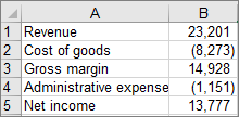
Select your data.

-
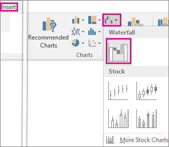
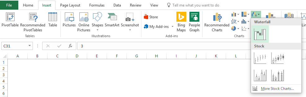
Click Insert > Insert Waterfall or Stock chart > Waterfall.
You can also use the All Charts tab in Recommended Charts to create a waterfall chart.
Tip: Use the Design and Format tabs to customize the look of your chart. If you don’t see these tabs, click anywhere in the waterfall chart to add the Chart Tools to the ribbon.

Start subtotals or totals from the horizontal axis
If your data includes values that are considered Subtotals or Totals, such as Net Income, you can set those values so they start on the horizontal axis at zero and don’t «float».
-
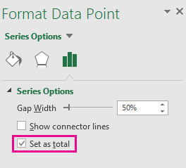
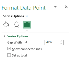
Double-click a data point to open the Format Data Point task pane, and check the Set as total box.
Note: If you single-click the column, you’ll select the data series and not the data point.
To make the column «float» again, uncheck the Set as total box.
Tip: You can also set totals by right-clicking on a data point and picking Set as Total from the shortcut menu.
Show or hide connector lines
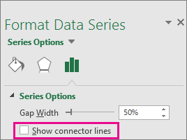
Connector lines connect the end of each column to the beginning of the next column, helping show the flow of the data in the chart.
-
To hide the connector lines, right-click a data series to open the Format Data Series task pane, and uncheck the Show connector lines box.
To show the lines again, check the Show connector lines box.
Tip: The chart legend groups the different types of data points in the chart: Increase, Decrease, and Total. Clicking a legend entry highlights all the columns that make up that group on the chart.
Here’s how you create a waterfall chart in Excel for Mac:
-
Select your data.
-
On the Insert tab on the ribbon, click
(Waterfall icon) and select Waterfall.Note: Use the Chart Design and Format tabs to customize the look of your chart. If you don’t see these tabs, click anywhere in the Waterfall chart to display them on the ribbon.
 (Waterfall icon) and select Waterfall.
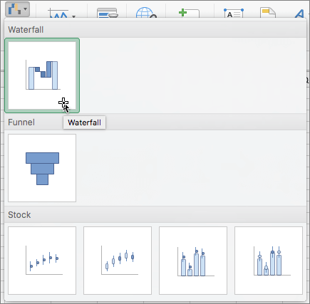
Waterfall charts are a powerful tool for visualizing changes in data over time. From analyzing financial statements to tracking project progress, waterfall charts can provide valuable insights into complex datasets. Excel is a popular solution for creating waterfall charts, but many users struggle to create charts that are both visually appealing and easy to understand.
In this step-by-step guide, you’ll learn how to create an impressive waterfall chart in Excel that will help you communicate your data effectively. Whether you’re a beginner or an experienced Excel user, our guide provides all the necessary tips and tricks to create a stunning waterfall chart that will impress your audience. So let’s dive in and learn how to create an eye-catching waterfall chart in Excel!
Waterfall charts 101
A waterfall chart (also known as a cascade chart or a bridge chart) is a special kind of chart that illustrates how positive or negative values in a data series contribute to the total. In other words, it’s an ideal way to visualize a starting value, the positive and negative changes made to that value, and the resulting end value. In a waterfall chart, the first column is the starting value and the last column is the end value. The floating columns between them are the contributing positive or negative values.
Note: Other fun names for waterfall charts include Mario chart and flying bricks chart, because individual chart elements resemble an old arcade game.
Some people like to connect the lines between the contributions to make the chart look like a bridge (giving us the bridge chart name), while others leave the columns floating.
Uses of waterfall charts
Waterfall charts are popular in the corporate and financial environment because they are very useful for a visualization of the positive and negative movements within a measured quantity or KPI, such as your Monthly Net Profit or Cash Flow.
Other examples of quantitative analyses, where waterfall charts are used, include:
- Visualizing profit and loss statements
- Comparing product earnings
- Highlighting budget changes on a project
- Analyzing inventory or sales over a period of time
- Showing product value over a period of time
- Creating executive dashboards
In a nutshell, use a waterfall chart whenever you want to show how a starting value increases or decreases through a series of positive or negative changes.
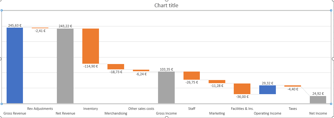
Tip: While the most typical waterfall chart is the one with a starting and ending value, you can also create subtotals as visual milestones in the series. These show up as full columns. For example, you might want to use Net revenue and Gross Income as two checkpoints between Gross Revenue and Net income starting and ending values.
How to create a waterfall chart in Excel
Before Office 2016, creating waterfall charts in Excel was a notoriously difficult process. Note that I used the word «creating» and not «inserting». That’s right — you did not insert a waterfall chart, you created it.
Let’s start with the process of creating a waterfall chart👇
The easiest way:
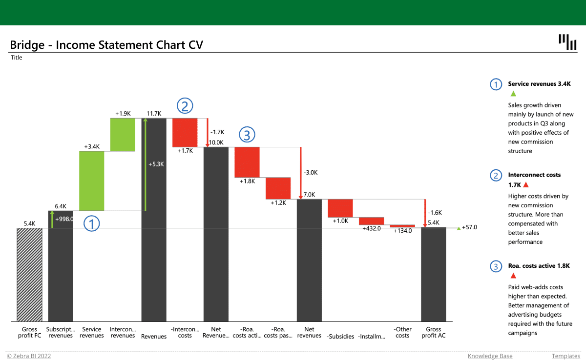
This is what your waterfall chart could look like in just a couple of clicks:
Amazing, right?
If you don’t have time to tweak the default Excel waterfall charts, as explained further in the guide, and would like to add those advanced features to your waterfall charts fast, Zebra BI for Office is just what you need. See just how easy creating a waterfall chart can be:
Compared to the other methods explained, this looks so easy it’s scary! By the way, you can do this in Office 2019 and 2021, Office 365, and Office for Mac! It’s also possible to do the same thing in PowerPoint, too.
Zebra BI for Office is already available in Excel. Download the sample file and follow the instructions that will help you get started.
Get started
download
And now, let’s check how to do it with the native Excel charts👇
Excel 2016 way:
Microsoft decided to listen to user feedback and introduced 6 highly requested charts in Excel 2016, including a built-in Excel waterfall chart.
No more templates, additional series, formulas, or tinkering with the charts. Just 2 clicks and your awesome waterfall chart is inserted.
Or is it? 🤨
While the addition of waterfall charts in Excel 2016 is a great step forward, the current functionality still leaves much to be desired.
10 steps to a perfect Excel waterfall chart
Here are some ways that can help you create better Excel waterfall charts and some things that are still missing. If you change your mind and want to do it easier, just download our free template and save your time for some better things.
1. Remember to set the totals
Let’s say we want to have this data table visualized with a waterfall chart: EBITDA of our fictional company for the years 2015, and 2016 and the individual contributions of 7 small business units to the change from 2015 to 2016.
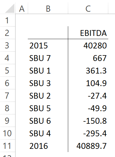
This shouldn’t be too hard. Click inside the data table, go to the «Insert» tab and click «Insert Waterfall Chart» and then click on the chart. Voila:
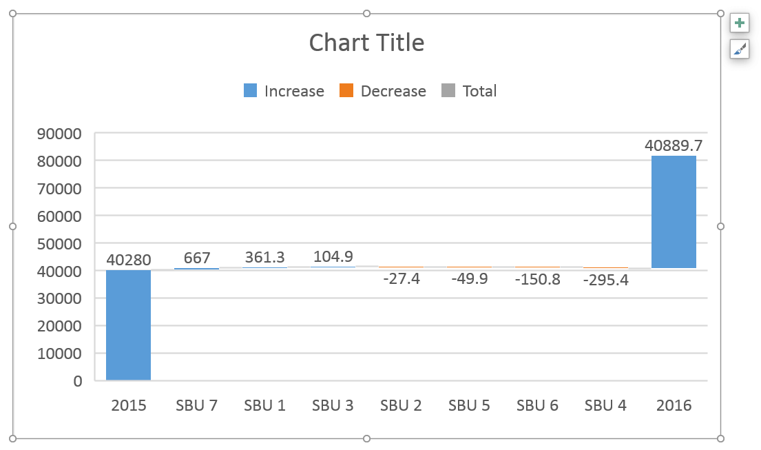
OK, technically this is a waterfall chart, but it’s not exactly what we hoped for. In the legend we see Excel 2016 has 3 types of columns in a waterfall chart:
- Increase
- Decrease
- Total
This is correct, but in the chart, there are no Total columns, only Increase and Decrease. The first and last columns should be Total (start on the horizontal axis) and to set them as such, we have to double-click on each of them to open the Format Data Point task pane and check the Set as total box.

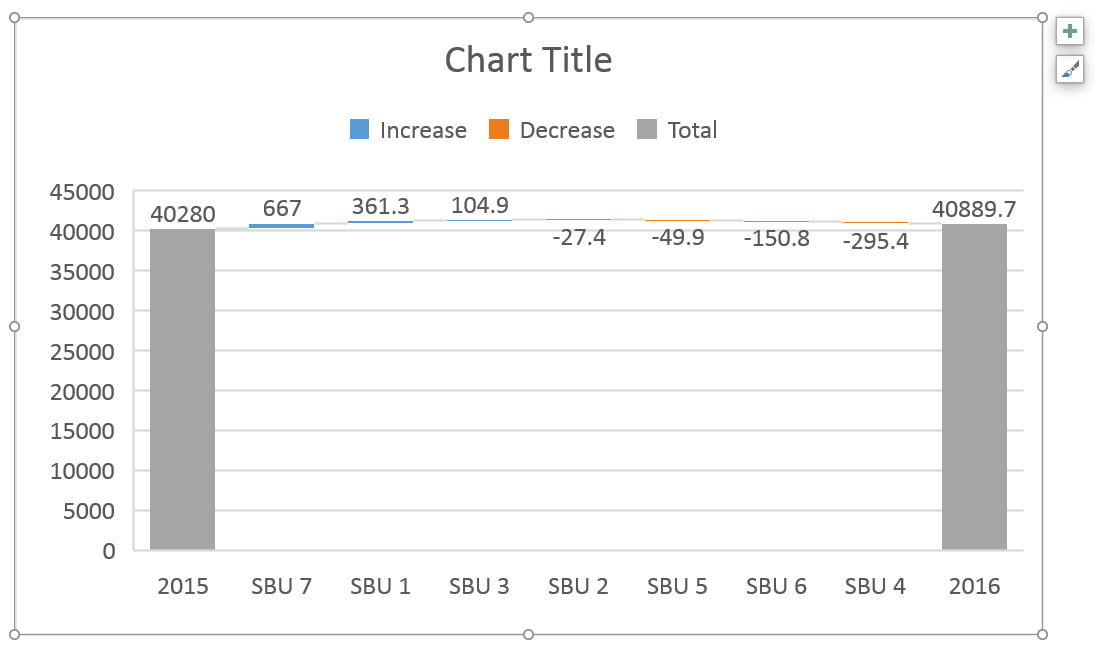
You can also right-click the data point and select Set as Total from the list of menu options.
Or, you can skip all this and use Zebra BI for Office to do the hard work for you.
Finally, we have our waterfall chart:
2. Ditch the clutter on your visualization
Data visualization best practice is to remove ALL elements from the visualization that is not absolutely necessary (if you’re interested, you can learn more about this in our free webinar: Data visualization in depth).
Similar to other Excel charts, the default Excel waterfall chart also suffers from having too much clutter. The legend, the vertical axis, and labels, the horizontal grid lines — none of them contribute to the reader’s better understanding of the data. If anything, they are a distraction.
So, let’s remove all unnecessary elements and write our key message to the title. It’s a shame that the chart title cannot be inserted automatically from a cell.
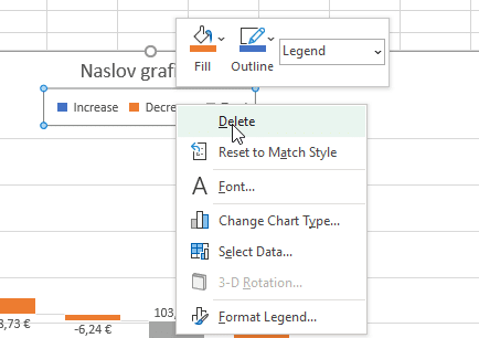
Tip: To remove the distracting chart elements, right-click on each of them and then click «Delete«.
Great, this is much better. But it required additional work that would not be required if Excel defaults were better. We’ll show you how to do it better in Zebra BI for Office.
3. Break the axis to highlight contributions
This limitation is especially noticeable in waterfall charts because waterfall charts have essentially two different types of data:
- Totals: usually the first and last column in a series.
- Contributions: the floating bricks make up the “bridge” between the two totals.
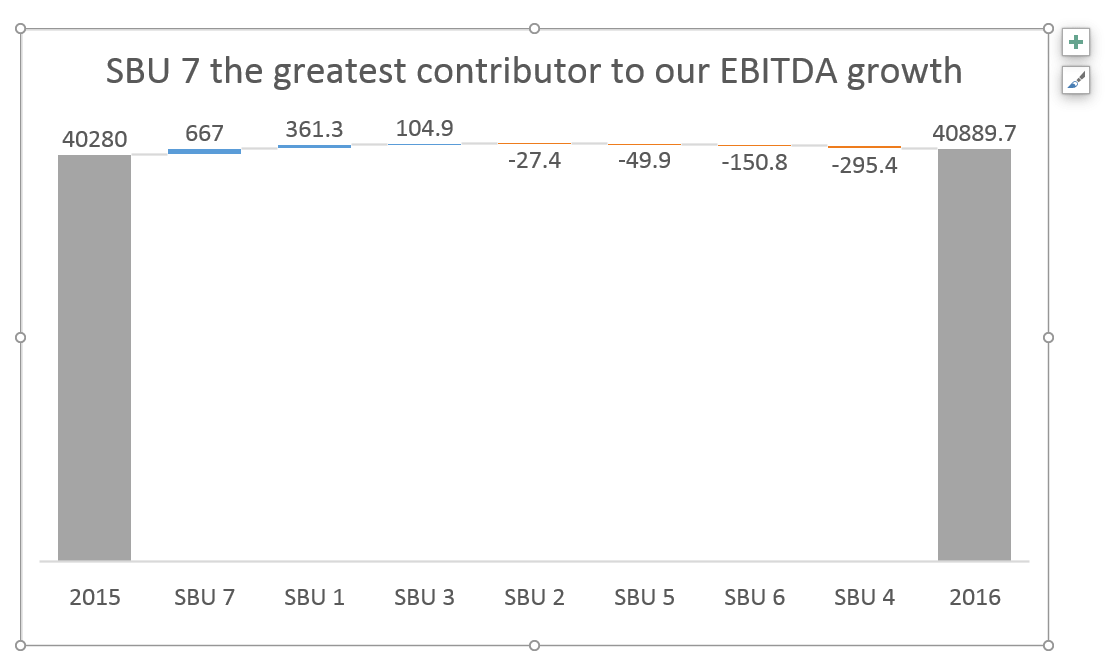
A common problem is that contributions are often very small compared to totals. This is also apparent in our example (see the image above).
First, a point of order: this chart correctly visualizes the situation as the contributions really ARE that small compared to totals. Our 2016 result is essentially the same as our 2015 result.
This visualization is also completely in line with IBCS Standards.
However, users (and their bosses) are sometimes more interested in contributions than in totals and the relationship between the two.
In this case, the only viable option would be to break the vertical axis and have the totals start at some value larger than 0. Let’s say 35,000. This highlights individual contributions, but risks guiding unaware readers to false conclusions about the data.
You can again resort to using tutorials:
- http://peltiertech.com/broken-y-axis-in-excel-chart/
- http://www.tushar-mehta.com/excel/newsgroups/broken_y_axis/tutorial/index.html
Another, somewhat simpler option is to do the following:
- Click on the chart to select it
- Re-add vertical axis: Go to Design >> Add Chart Element >> Axes >> Primary Vertical
- «Break» vertical axis: right click on the vertical axis and click «Format Axis…«, then under Axis Options write «35000» under Bounds >> Minimum.
- Remove the vertical axis: right click on the vertical axis and click «Delete«
This is the chart we end up with:
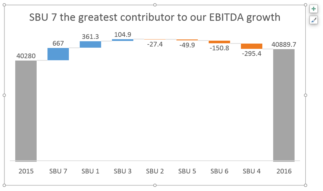
Now the contributions are much more prominent, but there’s no obvious indication that the vertical axis does not start at zero which is really bad because the user does not draw the correct conclusion from the visualization.
4. Add relative contributions in percentages
When analyzing contributions you’re sometimes more interested in relative contributions (in percentages of the total) than in absolute contributions.
Unfortunately, if you want to do that in a default Excel waterfall chart, you’re out of luck — you’re stuck with displaying absolute contributions only.
✔️ Look to the end of the article to see how easy this is to do in Zebra BI for Office.
5. Highlight differences between totals
Another thing that you’re not able to do in an Excel waterfall chart is to display the total difference between 2015 and 2016 in our example.
Sure, you can see in the chart that the 2016 column is higher than the 2015 column (especially now that we cut the vertical axis). But by how much? Unless you can do complex subtractions in your head, you don’t know the exact number. There’s also no way to display the relative difference in percentage.
Since this difference between totals is rather important, it’s definitely a major feature that’s missing in Excel waterfall charts.
✔️ Of course, it’s much easier to highlight the differences in Zebra BI for Office.
6. Use vertical waterfall charts
We know from the How to Choose the Right Business Chart article that horizontal charts (i.e. the charts that have a horizontal category axis) are used to display time-related data. For everything else, we should use vertical charts instead.
Waterfall charts are no exception. Strangely, in Excel 2016, there is no way to insert a vertical waterfall chart. While this feature has been requested, there’s no indication of whether it will be implemented and when.
✔️ We prepared a demonstration in Zebra BI for Office, so you can see how to create an income statement with vertical waterfall charts.
7. Add (some) subtotals
Since we’re on the subject of visualizing income statements — in a typical income statement, there are some categories that are actually sums of several other categories.
For example, you can choose to calculate a sum of all Operating Expenses (OpEx). This better visualizes the relationship between «Revenue» and «Earnings before interest and taxes» (EBIT). EBIT = Revenue — OpEx.
In a table, this is easy to do — just write a formula and you’re done.
When you create a waterfall chart in Excel? Not so much. It’s apparently so hard to do it manually that there’s not a single tutorial or template available on the internet.
You can, however, enter subtotals and designate them as such in your waterfall chart. However, you need to calculate them yourself to make sure they are correct.
✔️ You can see how Zebra BI for Office automatically creates subtotals in this handy animated gif at the end of this article.
8. Customize your chart with colors
The default color scheme in Excel could be better. Visit the Chart Design tab and open the Change Colors gallery.

Here, you can select a color palette. You can also choose a different theme on the Page Layout tab. To adjust how the colors are used, click the Colors button and select Customize Colors at the bottom of the list.

You can set it up to display positive values in green and negative values in red, which is a common approach in financial reporting.
9. Turn connector lines on or off
Connector lines connect columns to show the movements in values in the chart. You can turn them on or off by right-clicking a data series to open the Format Data Series pane, and checking/unchecking the Show connector lines box.
10. Scale your charts
Finally, we arrive at one major feature that’s missing in Excel from the very beginning: scaling multiple charts.
While this problem is not limited to waterfall charts, it’s too important not to mention it here.
Making sure that all related charts in a report or dashboard are on the same scale is one of the most important concepts in data visualization.
If you don’t synchronize scales, don’t even insert the charts
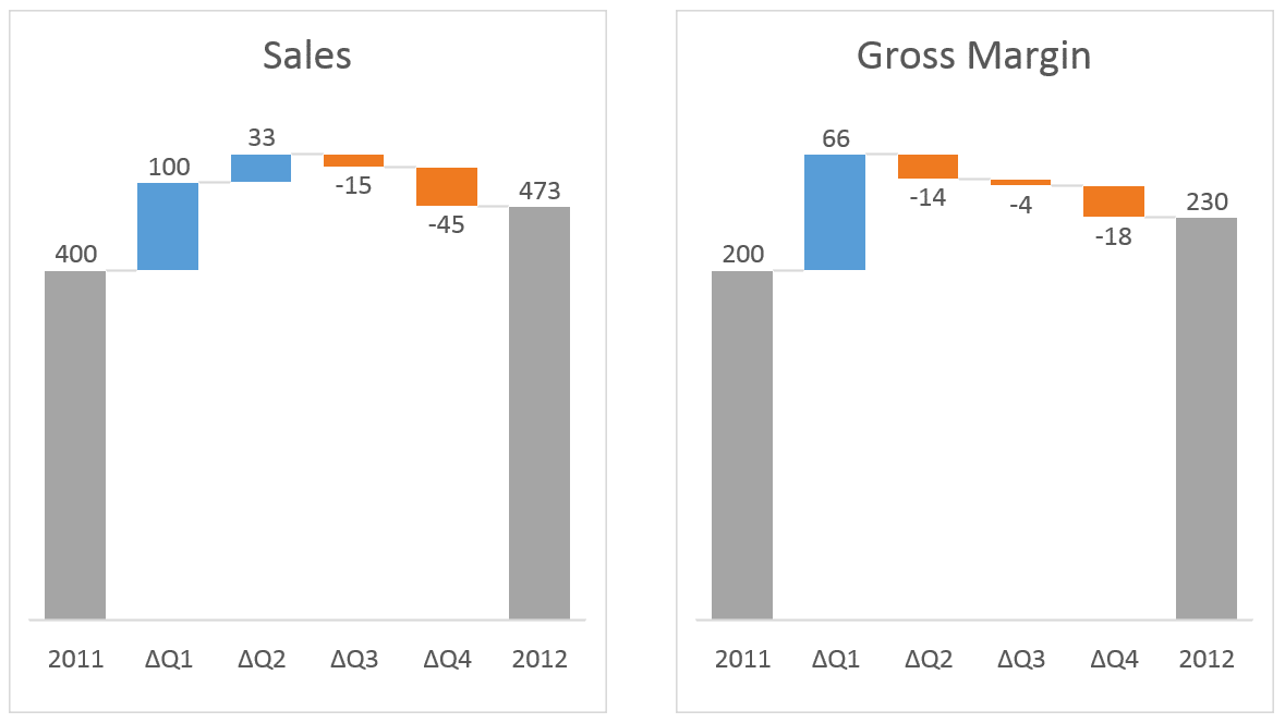
All too often you see two Excel charts side by side with completely different scales. While each of them is an adequate data visualization on its own, you must make sure they are scaled once you put them side by side! Otherwise don’t even insert the charts and just leave the data in a table — or risk misleading/incorrect interpretation.
So, how do you synchronize scales of Excel charts? While the procedure is not particularly hard, it is time-consuming. It’s a similar procedure that we used to break the axis.
Say we have these two default Excel waterfall charts and we need to scale them:
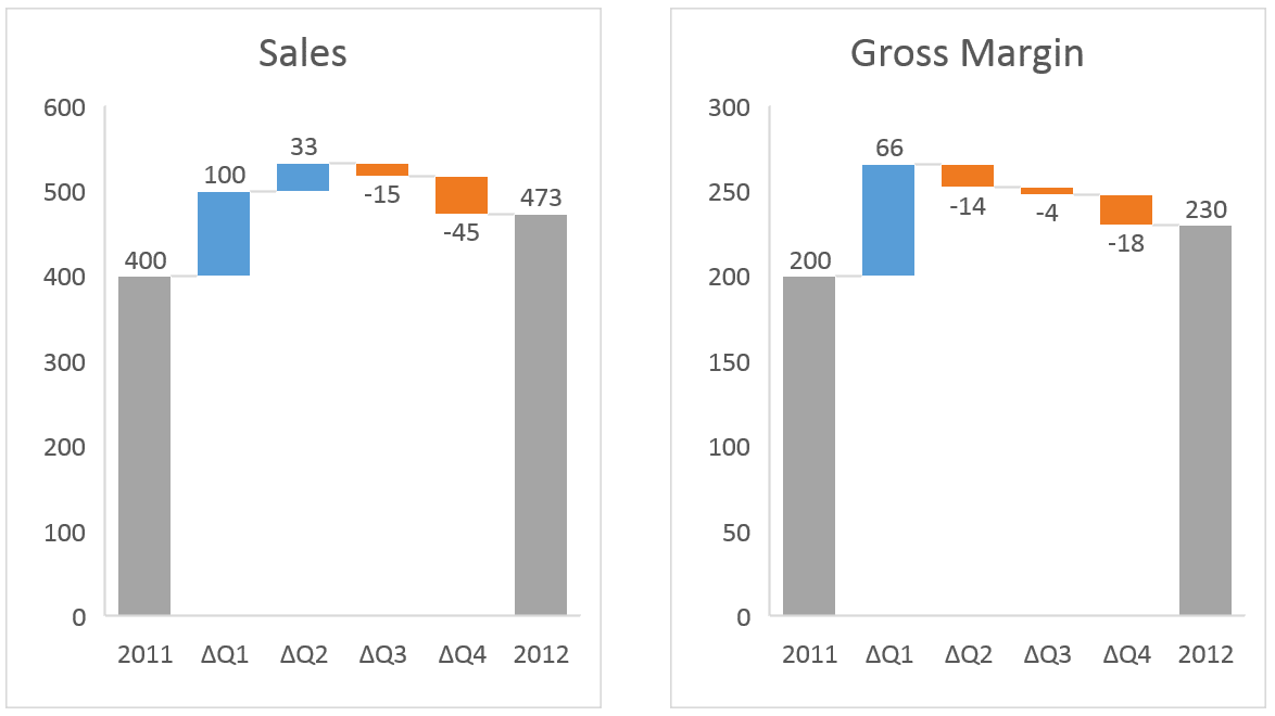
The first step is to re-add Vertical Axis on both charts.
- Click on the first chart to select it
- Re-add vertical axis: Go to Design >> Add Chart Element >> Axes >> Primary Vertical
- Repeat for the second chart
This is what we have so far:
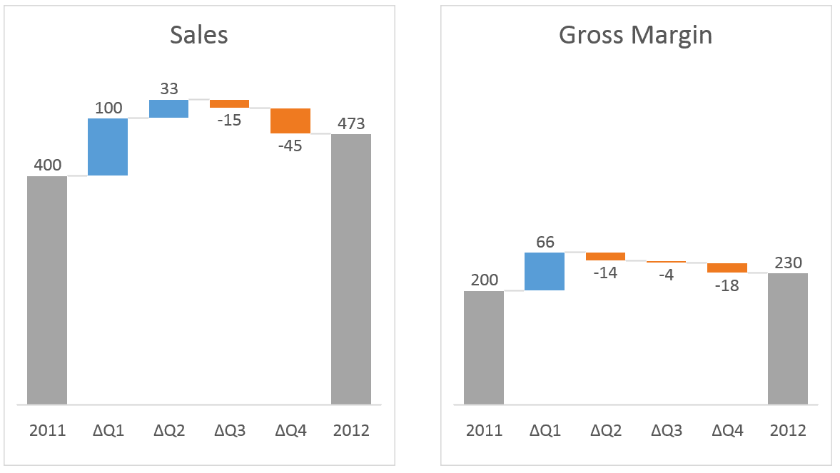
Now we have to adjust the scale of the right chart to be the same as the left. Right-click on the vertical axis and click «Format Axis…», then under Axis Options write «600» under Bounds >> Minimum.
Remove the vertical axis from both charts (right-click on the vertical axis and click «Delete«) and we have our correct visualization:
OK, that wasn’t too bad. Now, what if you have a monthly report with 6 waterfall charts on it? Would you do this procedure for 6 charts every month when the data changes? I guess not.
Of course, you can automate this, but you have to use VBA to do it. If you don’t want to use VBA, maybe this article from 2012 by Jon Peltier will help you.
Some more advanced things you can do much easier
You got it so far: everything is much easier if you use Zebra BI for Office instead of native Excel charts. See what else can be done 👇
Adding variances and difference highlights
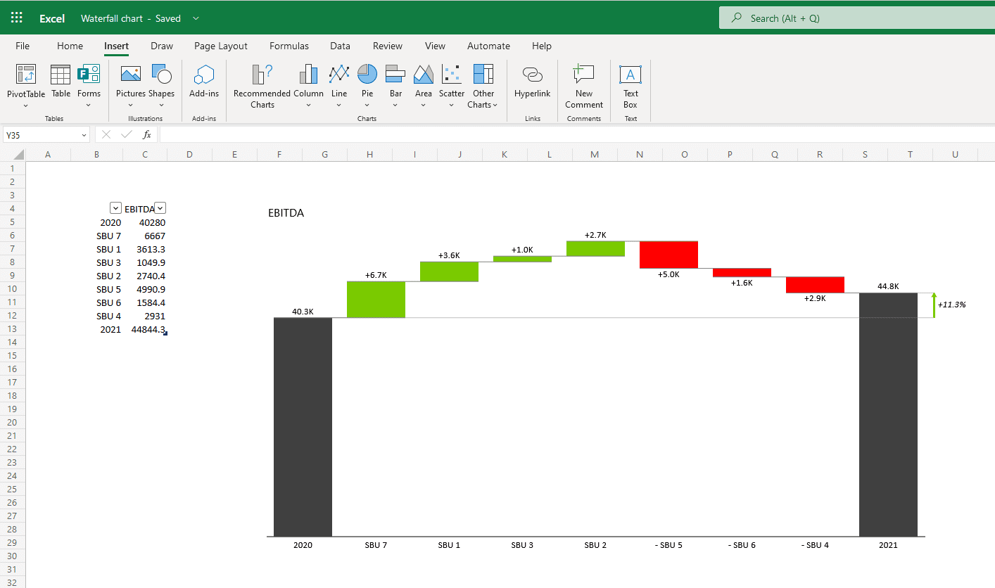
The default Excel waterfall charts do not show a very important feature that is crucial for the understanding of your performance: variances (absolute & relative) and difference highlights. In Zebra BI for Office, both features are applied automatically.
You can also control whether an increase is a positive or a negative event. We know that in some cases, like when it comes to costs, an increase is a negative development. You can simply right-click on the category where data should be inverted and select a custom calculation «Invert». This will automatically adapt the visualization to display the right context.
Another useful feature we added is the difference highlights between starting and ending values. The difference highlight is added automatically and is on by default. By going to the settings in the global toolbar, you can also switch it off.
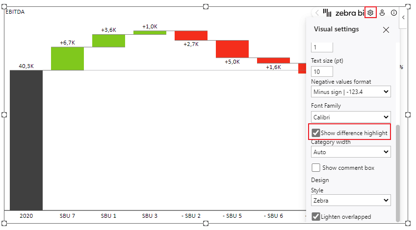
In the previous example, you can see that the increase between EBITDA in 2020 and 2021 was 4.6k or 11.3%.
Creating an income statement with vertical waterfall charts
How about inserting a waterfall chart into an income statement? With the Zebra BI Tables for Office add-in, this is just a few clicks away.
The cool thing about this is that by glancing at the waterfall chart, you can already see how you’re performing. The calculations like «Result» and «Invert» are reflected in the waterfall chart and all categories get subtracted so that you can clearly see the contribution of each to the final result.
Small multiples with waterfall charts
How about creating up to 200 waterfall charts at once?
Here are 6 waterfall charts in a few clicks:
You only need to select a single cell in your data and insert the Zebra BI Charts for Office add-in. Use the chart slider to get to the waterfall chart, use the custom calculation «Result» on the first and last entry, and Zebra BI will do the rest.
You will see the automatically calculated variances and highlighted differences. But, most importantly, no matter how many charts you have, they are all inserted within the same visual and also automatically scaled between each other which immediately puts the data into the right perspective.
Check this short video to see how easy is to create Waterfall charts with Zebra BI for Office:
Все чаще и чаще встречаю в отчетности разных компаний и слышу просьбы от слушателей на тренингах объяснить как строится каскадная диаграмма отклонений — она же «водопад», она же «waterfall», она же «мост», она же «bridge» и т.д. Выглядит она примерно так:
")
Издали действительно похожа на каскад водопадов на горной реке или навесной мост — кто что видит 
Особенность такой диаграммы том, что:
- Мы наглядно видим начальное и конечное значение параметра (первый и последний столбцы).
- Положительные изменения (рост) отображаются одним цветом (обычно зеленым), а отрицательные (спад) — другим (обычно красным).
- Иногда в диаграмме могут присутствовать ещё и столбцы промежуточных итогов (серые, приземленные на ось Х столбцы).
В повседневной жизни такие диаграммы используются обычно в следующих случаях:
- Наглядное отображение динамики какого-либо процесса во времени: потока наличности (cash-flow), инвестиций (вкладываем деньги в проект и получаем от него прибыль).
- Визуализация выполнения плана (крайний левый столбик в диаграмме — факт, крайний правый — план, вся диаграмма отображает наш процесс движения к желаемому результату)
- Когда нужно наглядно показать факторы, влияющие на наш параметр (факторный анализ прибыли — из чего она складывается).
Есть несколько способов построения такой диаграммы — всё зависит от вашей версии Microsoft Excel.
Способ 1. Самый простой: встроенный тип в Excel 2016 и новее
Если у вас Excel 2016, 2019 или новее (или Office 365), то построение такой диаграммы не составит труда — в этих версиях Excel такой тип уже встроен по умолчанию. Нужно будет лишь выделить таблицу с данными и выбрать на вкладке Вставка (Insert) команду Каскадная (Waterfall):

В результате мы получим практически готовую уже диаграмму:

Сразу же можно настроить желаемые цвета заливки для положительных и отрицательных столбцов. Удобнее всего это сделать, выделив соответствующие ряды Увеличение и Уменьшение прямо в легенде и, щёлкнув по ним правой кнопкой мыши, выбрать команду Заливка (Fill):

Если нужно добавить в диаграмму столбцы с промежуточными итогами или финальный столбец-итог, то удобнее всего это сделать с помощью функций ПРОМЕЖУТОЧНЫЕ.ИТОГИ (SUBTOTALS) или АГРЕГАТ (AGGREGATE). Они посчитает накопленную с начала таблицы сумму, исключив при этом из нее выше расположенные аналогичные итоги:

В данном случае, первый аргумент (9) — это код математической операции суммирования, а второй (0) заставляет функцию не учитывать в результатах уже вычисленные итоги за предыдущие кварталы.
После добавления строк с итогами останется выделить на диаграмме появившиеся итоговые колонки (сделать два последовательных одиночных щелчка по столбцу) и, щёлкнув правой кнопкой мыши, выбрать команду Установить в качестве итога (Set as total):

Выбранный столбец «приземлится» на ось Х и автоматически поменяет цвет на серый.
Вот, собственно, и всё — диаграмма-водопад готова:

Способ 2. Универсальный: невидимые столбцы
Если у вас Excel 2013 или более древние версии (2010, 2007 и т.д.), то описанный выше способ вам не подойдёт. Придется идти обходным путем и выпиливать недостающую каскадную диаграмму из обычной гистограммы с накоплением (суммированием столбиков друг на друга).
Хитрость тут заключается в использовании прозрачных столбцов-подпорок, приподнимающих наши красные и зеленые ряды данных на нужную высоту:

Для построения такой диаграммы нам потребуется добавить к исходным данным еще несколько вспомогательных колонок с формулами:

- Во-первых, нужно разделить наш исходный столбец, выделив положительные и отрицательные значения в разные колонки с помощью функции ЕСЛИ (IF).
- Во-вторых, нужно будет добавить перед сделанными столбцами колонку Пустышки, где первое значение будет 0, а начиная со второй ячейки формулой будет вычисляться высота тех самых прозрачных подпирающих столбцов.
После этого останется выделить всю таблицу кроме исходного столбца Поток и создать обычную гистограмму с накоплением через Вставка — Гистограмма (Insert — Column Chart):

Если теперь выделить синие столбцы и сделать их невидимыми (по ним правой кнопкой мыши — Формат ряда — Заливка — Нет заливки), то мы как раз и получим то, что требуется.
В плюсах подобного способа — простота. В минусах — необходимость считать вспомогательные колонки.
Способ 3. Если уходим в минус — всё сложнее
К сожалению, предыдущий способ адекватно работает только для положительных значений. Если хотя бы на каком-то участке наш водопад уходит в отрицательную область, то сложность задачи возрастает в разы. В этом случае необходимо будет формулами просчитать каждый ряд (пустышки, зеленые и красные) отдельно для отрицательной и положительной частей:

Чтобы не сильно мучиться и не изобретать велосипед, готовый шаблон для такого случая можно скачать в заголовке этой статьи.
Способ 4. Экзотический: полосы повышения-понижения
Этот способ основан на использовании специального малоизвестного элемента плоских диаграмм (гистограмм и графиков) — Полос повышения-понижения (Up-Down Bars). Эти полосы попарно соединяют точки двух графиков, чтобы наглядно показать какая из двух точек выше-ниже, что активно используется при визуализации план-факта:

Легко сообразить, что если убрать линии графиков и оставить на диаграмме только полосы повышения-понижения, то мы получим все тот же «водопад».
Для такого построения нам потребуется добавить к нашей таблице еще два дополнительных столбца с простыми формулами, которые расчитают положение двух требуемых невидимых графиков:

Для создания «водопада» нужно выделить столбец с месяцами (для подписей по оси Х) и два дополнительных столбца График 1 и График 2 и построить для начала обычный график через Вставка — График (Insert — Line Сhart):

Теперь добавим к нашей диаграмме полосы повышения-понижения:
- В Excel 2013 и новее для этого необходимо выбрать на вкладке Конструктор команду Добавить элемент диаграммы — Полосы повышения-понижения (Design — Add Chart Element — Up-Down Bars)
- В Excel 2007-2010 — перейти на вкладку Макет — Полосы повышения-понижения (Layout — Up-Down Bars)
Диаграмма после этого начнёт выглядеть примерно так:

Осталось выделить графики и сделать их прозрачными, щелкнув по ним по очереди правой кнопкой мыши и выбрав команду Формат ряда данных (Format series). Аналогичным образом можно изменить и стандартные, весьма убого выглядящие, чёрно-белые цвета полос на зелёные и красные, чтобы получить в итоге более приятную картинку:

В последних версиях Microsoft Excel ширину полос можно изменить, щёлкнув по одному из прозрачных графиков (не по полосам!) правой кнопкой мыши и выбрав команду Формат ряда данных — Боковой зазор (Format series — Gap width).
В старых версиях Excel для такого исправления приходилось использовать команду на Visual Basic:
- Выделите построенную диаграмму
- Нажмите сочетание клавиш Alt+F11, чтобы попасть в редактор Visual Basic
- Нажмите сочтетание клавиш Ctrl+G, чтобы открыть панель прямого ввода команд и отладки Immediate (обычно она расположена внизу).
- Скопируйте и вставьте туда вот такую команду: ActiveChart.ChartGroups(1).GapWidth = 30 и нажмите Enter:

При желании можно, конечно, поиграться со значением параметра GapWidth, чтобы добиться нужной величины зазора:

Ссылки по теме
- Как в Excel построить диаграмму-шкалу (bullet chart) для визуализации KPI
- Новые возможности диаграмм в Excel 2013
- Как в Excel создать интерактивную «живую» диаграмму
The Definitive Guide to Creating a Waterfall Chart
Smartsheet Contributor
Kate Eby
March 4, 2016
No matter what industry you work in, at some point you will need to analyze a value over time like yearly sales, total profit, or inventory balance. When doing so, it is helpful to see where you started and how you arrived at the final value. A waterfall chart is an ideal way to visualize a starting value, the positive and negative changes made to that value, and the resulting end value.
Using a template is the easiest way to create a waterfall chart. In this article, you’ll find the best Excel waterfall chart template and we’ll show you how to customize the template to fit your needs. Plus, we’ll give you step-by-step instructions to create a waterfall chart in Excel, from scratch.
You’ll also learn how to create a waterfall chart using Smartsheet, a spreadsheet-inspired work management tool that provides real-time visualization that dynamically updates as values are changed.
What Is a Waterfall Chart?
A waterfall chart is also known by many other names: waterfall graph, bridge graph, bridge chart, cascade chart, flying bricks chart, Mario chart (due to its resemblance to the video game), and net profit waterfall chart. Regardless of the name, this versatile chart is a great way to provide a quick visual into positive and negative changes to a value over a period of time.
Within a waterfall chart, the initial and final values are shown as columns with the individual negative and positive adjustments depicted as floating steps. Some waterfall charts connect the lines between the columns to make the chart look like a bridge, while others leave the columns floating.
Waterfall charts became popular in the late 20th century, when the management consulting organization McKinsey & Company used them in presentations to clients. Then McKinsey associate Ethan M. Rasiel made them widely popular in corporate analysis in his 1999 book, The McKinsey Way.
The key feature of a waterfall chart, per Rasiel, is that it shows changes not only over time, but in relation to the previous period or other milestone of measurement. Each step in the waterfall gets you to the final result and demonstrates how you got there. And the beauty of a waterfall chart is its simplicity of construction, even in analyzing complex information — which means it will likely enjoy heavy use into the future.
When to Use a Waterfall Chart?
Waterfall charts are helpful for a variety of scenarios, from visualizing financial statements to navigating large amounts of census data. Here are some examples of situations where you might want to use a waterfall chart:
- Evaluating company profit.
- Comparing product earnings.
- Highlighting budget changes on a project.
- Analyzing inventory or sales over a period of time.
- Showing product value over a period of time.
- Visualizing profit and loss statements.
- Creating executive dashboards.
- Tracking consulting jobs.
- Keeping track of retail inventory.
- Documenting contracts.
- Demonstrating how operating costs have changed from one time period to another.
- Contrasting competitors.
Who Typically Uses a Waterfall Chart?
Waterfall charts began as a way to track monetary performance over time and have become a mainstay among financial industries and departments. However, more and more industries, as well as departments within those industries, are finding it useful to adopt waterfall charts to track and present performance. These include the following:
- Sales companies and teams
- Developers and IT professionals
- Retailers and ecommerce companies
- Legal departments and lawyers
- Construction companies
- Educators and exam-scoring companies
The Benefits of Using a Waterfall Chart
Waterfall charts are a simple visual format that presents your data in an impactful manner, which is why they have become increasingly popular in recent years. There are other benefits of using waterfall charts as well. Here are some examples of advantages you can enjoy:
- Customize the appearance of your waterfall charts, as you would with any other chart.
- Make them as simple and bare-bones or as complex as you like.
- Deploy them for analytical purposes, especially to explain or present the gradual changes in the value of an item.
- Study a wide variety of data, such as inventory analysis or performance analysis.
- Demonstrate how you have arrived at a net value, by breaking down the cumulative effect of positive and negative contributions.
The Challenges in Using a Waterfall Chart
That said, there have been and continue to be challenges in creating and using waterfall charts. Some of the roadblocks users have encountered include the following:
- Before Office 2016, creating waterfall charts in Excel was very difficult and labor-intensive. The instructions below are for editions before Office 2016; the PowerPoint instructions are for 2016 and later editions.
- It can take a lot of input work to set totals.
- There’s a lot of unnecessary data and content around and on the chart.
- It takes too many clicks to break the axis.
- It’s not possible to display relative contributions in percentages.
- There’s no difference in the highlights.
- You can’t create a vertical Excel waterfall chart.
- They don’t allow subtotals.
- Scaling multiple charts is time-consuming.
The Typical Features of a Waterfall Chart
Each waterfall chart will have a slightly different appearance, depending on the type of data you choose to visualize. However, your final chart will likely include the following features:
- Floating Columns: To quickly provide a visual into the status of a value over time, the floating columns (also known as plot or plotted values) represent the positive and negative changes made to the initial value.
- Spacers: Because each of the columns in a waterfall chart don’t begin at zero, they need to be offset by a certain margin. This area is known as the spacer or padding.
- Connector Lines: The connector lines (also known as datum) show the relationships between the floating columns. Although they are not necessary for all waterfall charts, connector lines can be a helpful addition to improve the professional look of your chart.
- Color Coding: By assigning specific colors to the different column types, you can quickly tell positive from negative values and provide a quick visual of the movement over time.
- Crossover: There are some instances, depending on the values you’re plotting in your chart, where the values will move across the x-axis. For example, if you are creating a waterfall chart as a visual for a profit-and-loss statement and the first figure is 1,000 while the second figure is -2,000, part of the floating column will be above the x-axis and part will be below. This is an important feature of the waterfall chart, as the chart should adjust automatically to show movement across the axis.
Download Our Free Excel Waterfall Chart Template

The easiest way to assemble a waterfall chart in Excel is to use a premade template. A Microsoft Excel template is especially convenient if you don’t have a lot of experience making waterfall charts. All you need to do is to enter your data into the table, and the Excel waterfall chart will automatically reflect the changes.
Download Waterfall Template
Excel (2016/Office 365) | Excel (2010-2013) | Smartsheet
When adding your own data to the template, the waterfall chart will automatically update, but you may need to add or delete rows in your table depending on how much information you need to input. Adding or deleting rows could throw off your column formulas and totals. The solution is to copy the column formulas down to adjacent cells using the fill handle.
If you’re unsure how to fix the formulas as you add new rows, see below for “Step 2: Insert Formulas to Complete Your Table.”
After updating your waterfall chart to fit your needs, you can simply copy and paste it as an image into a PowerPoint presentation, dashboard, or report. Also, see the separate “How to Create a Waterfall Chart in PowerPoint” section below.
If you want to build a waterfall chart of your own, we’ve got the step-by-step instructions for you. Although Excel 2016 includes a waterfall chart type within the chart options, if you’re working with any version older than that, you will need to construct the waterfall chart from scratch.
Step 1: Create a data table
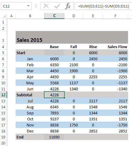
Let’s start with a simple table like annual sales numbers for the current year. You will see in the table below that the sales amounts vary for each month. Some months will have positive sales growth, while others will be negative.
- Insert three additional columns to your Excel table to represent the movement of the columns on the waterfall chart. The base column will represent the starting point for the fall and rise of the chart. You will input all the negative numbers from the sales flow in the fall column and all the positive numbers in the rise column.
*You will also want to add a Start and End row to your table to provide total values for the beginning and end of your sales year.
Step 2: Insert formulas to complete your table
The easiest way to complete your table is by adding formulas to the first cells in each of the corresponding columns and then copy them down to the adjacent cells using the fill handle.
- Select C4 in the Fall column and enter the following formula: =IF(E4<=0, -E4, 0)
*Drag the fill handle down to the end of the column to copy the formula.
- Select D4 in the Rise column and enter the following formula: =IF(E4>0, E4,0)
*Copy the formula down to the end of the table using the fill handle.
- Select B5 in the Base column and enter the following formula: =B4+D4-C5
*Use the fill handle to drag and copy the formula to the end of the column.
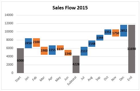
Step 3: Build a stacked column chart
Now you have all the necessary data to build your waterfall chart.
- Select the data you would like to highlight in your chart. Include the row and column headers, and exclude the sales flow column.
- Go to the Insert tab, click on the Column Charts group, and select Stacked Chart.
*Your stacked chart now appears in the worksheet, with all your data included, but it is not a waterfall chart just yet. Next, we will turn the stacked column chart into a waterfall chart.
Step 4: Convert your stacked chart to a waterfall chart
In order to make your stacked column chart look like a waterfall chart, you will need to make the Base series invisible on the chart.
- Click on the Base series to select them. Right-click and choose Format Data Series from the list.
- Once the Format Data Series pane appears to the right of your worksheet, Click on the Fill & Line icon (looks like a paint bucket).
- Select No fill in the Fill section and No line in the Border section.
- Now that the Base series is invisible, you should remove the Base label listed in the legend. To do this, double click on Base in the legend, right-click on the selected label, and click Delete from the dropdown list.
Step 5: Format your waterfall chart
To make your waterfall chart more engaging, let’s apply some formatting.
- Let’s start by color-coding the columns to help identify positive versus negative values. Select the Fall series in the chart, right-click and select Format Data Series from the list.
- Once the Format Data Series pane appears to the right of your worksheet, select the Fill & Line icon.
- Click on the color dropdown to select a color.
- Once you’ve picked the color for the Fall series, complete the same steps for the Rise series.
*You should also color-code the start and end columns to make them stand out, and will need to do those separately.
If you want to make your waterfall chart look a little nicer, remove most of the white space between the columns.
- Double-click on one of the columns in your chart.
- Once the Format Data Series pane opens up, change the Series Overlap to 100% and the Gap Width to 15%.
You’re almost finished. You just need to change the chart title and add data labels.
- Click the title, highlight the current content, and type in the desired title.
- To add labels, click on one of the columns, right-click, and select Add Data Labels from the list. Repeat this process for the other series.
- To format the labels, select one of the labels, right-click, and select Format Data Labels from the list.
- Once the Format Data Labels pane opens, you can adjust the label position, text color and font to make the numbers more readable.
*Once you’re done labeling the columns, you can delete unnecessary elements like zero values and the legend.
How to Add Subtotal or Total Columns
After completing your initial waterfall chart, you may decide to add a subtotal column to visualize status at a midway point. For example, in our sales flow example, it would be helpful to include a column showing mid-year sales.
- In your table, insert a row above July.
- Name the row Subtotal, and insert a formula to calculate total Rise for months Jan through Jun, minus total Fall for the same months.
- Next, you need to fill in the new subtotal column. Select the individual subtotal column in the waterfall chart. Right-click the column, select the Fill icon, and choose the color you would the column to be filled with.
Helpful Tips to Make Waterfall Charts
As you make more waterfall charts for more kinds of reports and data, there are some helpful tips that may come in handy.
- You’re allowed to enter two or more values into a column. If you have a column composed of more than one segment, you can enter an e (for “equals”) for, at maximum, one of them.
- For basic waterfall charts, every two columns are connected by only one horizontal connector. Select the connector, and it will show two handles.
- To change the column connections in the waterfall, drag the connectors’ handles.
- To start a new summation, remove the connector by deleting it. To add a connector, click Add Waterfall Connector in the context menu.
- Connectors may conflict with each other, which will result in skew connectors. You can resolve the problem by removing some of the skew connectors.
- To connect the “equals” column with the top of the last segment, drag the right handle of the highlighted connector.
- If you want to create a build-down waterfall chart, use the image toolbar icon.
- By using labels for level difference arrows, you’ll support the display of values as percentages of the 100%= value in the datasheet.
- Incorporate subtotals as a visual checkpoint in the chart.
- Customize the chart with logos, colors, etc., for maximum impact.
- Waterfall charts aren’t limited to financial analysis; they can also show user growth or any other changes in a vital base metric.
How to Create a Waterfall Chart in PowerPoint
It used to be a ponderous, difficult process to create or embed a waterfall chart in PowerPoint, but thankfully it’s now much easier in Office 365 and editions of PowerPoint 2016 and later. You’ll still need to use Excel to create the chart and values, but that functionality is built right into the newer editions of PowerPoint. Here’s how you do it.
Open a new PowerPoint presentation, and add a new blank slide after the title slide. Alternatively, you can work on a deck you’ve already started, but add a new slide where the waterfall chart will go.
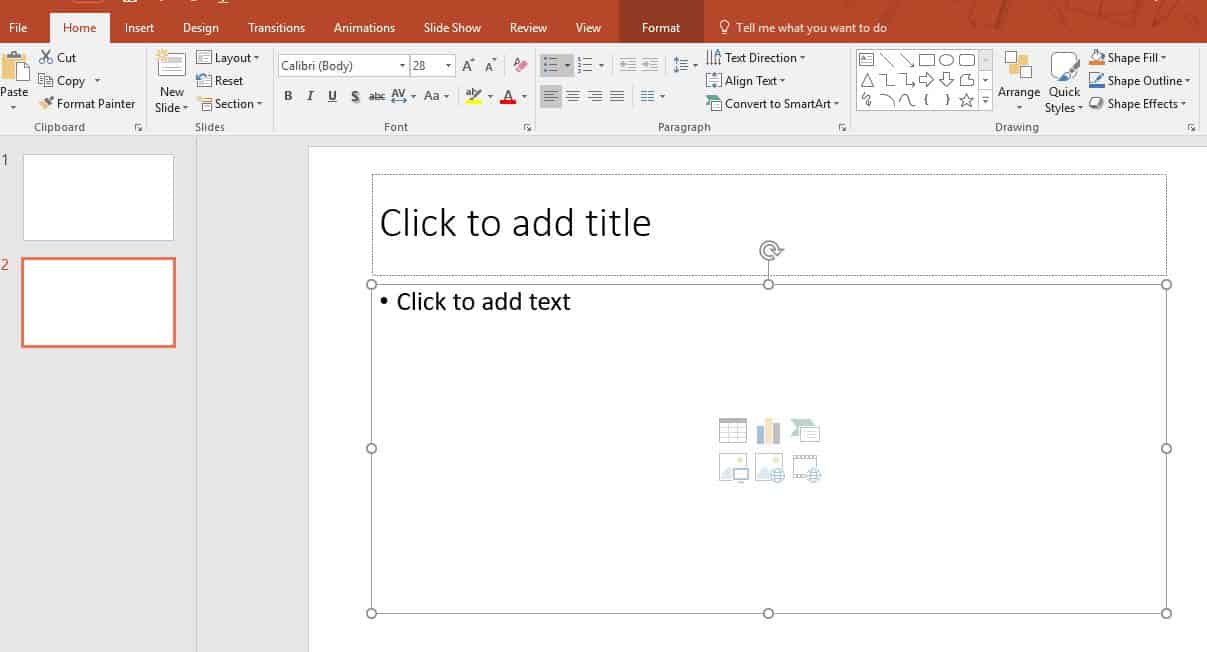
On the Insert tab, click the Chart icon in the middle of the top ribbon. On the left-hand menu, select Waterfall near the bottom.
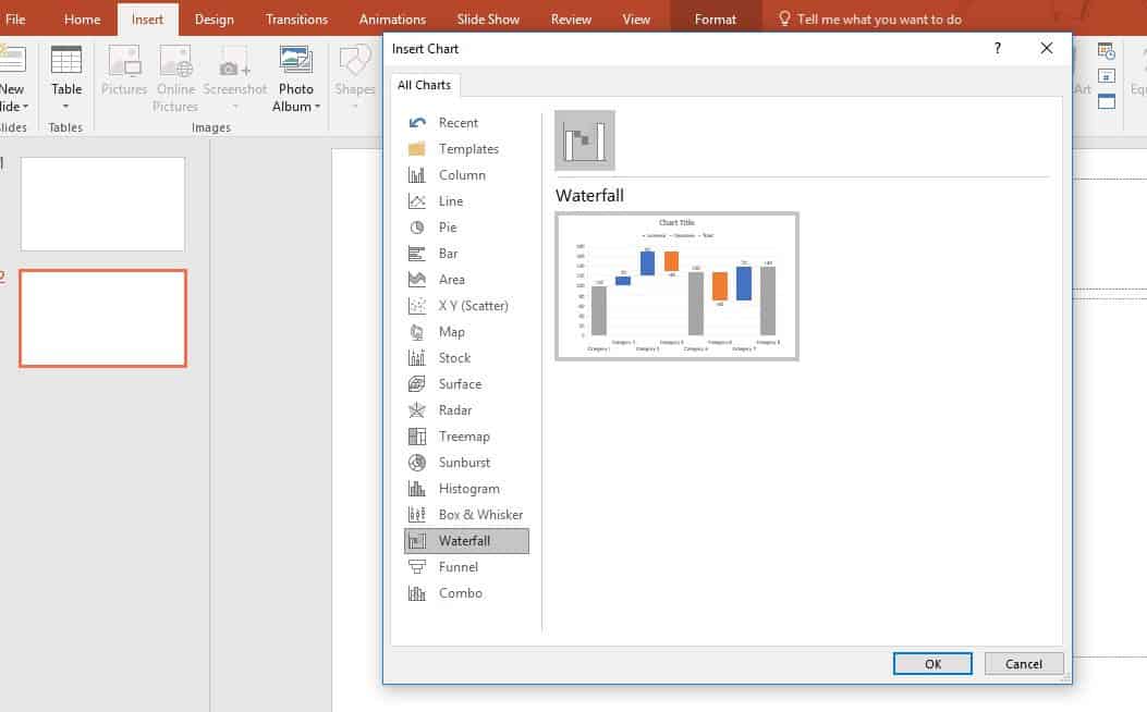
The slide will then be populated with a placeholder chart, and an Excel sheet will pop up.
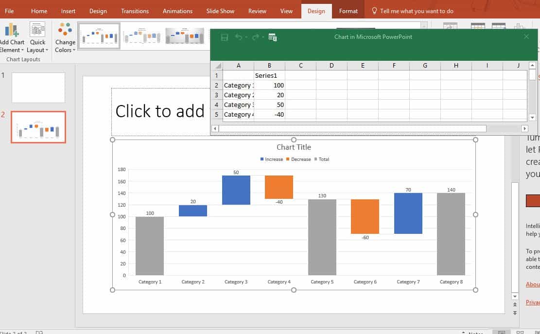
From there, add the values per the instructions for Excel above. The presentation of the blank chart is fairly intuitive to follow. The template has eight fields for measurement, but you can add more. Here, we have changed Category to the name of a month, showing eight months in a year.
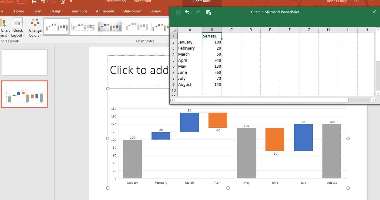
From there it’s easy to add the values for each category (in this case, month), and Excel will automatically update the working chart on the PowerPoint slide.
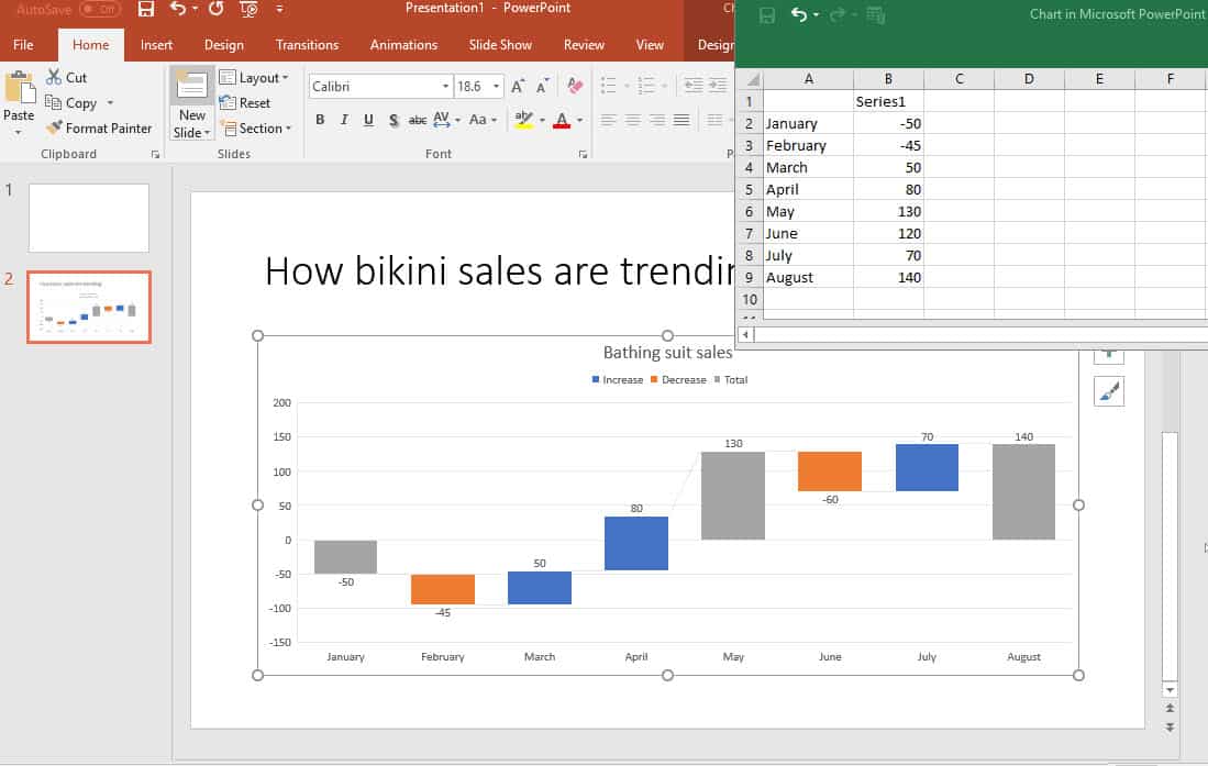
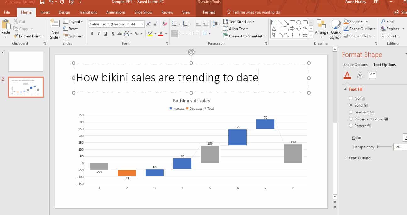
After you’ve adjusted and added all the values, you can close the Excel window, and the slide will graphically capture the final trends you’ve entered. You will see an area on the right where you can experiment with customization, colors, and other stylings, if desired.
A More Collaborative Waterfall Chart
Now that you’ve seen what it takes to construct a waterfall chart in Excel, I think we can agree that there is a lot to remember.
While a waterfall chart in Excel provides a way to visualize the change in value over a period of time, it doesn’t provide real-time visualization that dynamically updates as values are changed.
Luckily we have another, more collaborative way to create a waterfall chart using Smartsheet and the Microsoft Power BI integration.
How to Create a Waterfall Chart in Smartsheet
Smartsheet is a spreadsheet-inspired work management tool with robust collaboration and communication features. Smartsheet has a similar look and feel as Excel, so it’s easy to start using right away yet it’s cloud-based so you can access your data and information anywhere, anytime.
Let’s create a waterfall chart in Smartsheet.
Step 1: Create a simple table in Smartsheet
- To get started with Smartsheet, log in to your account and navigate to the Home tab.
- Click Create New, choose Blank Sheet, and name your new sheet Sales Flow 2015.
- Next, create the simple sales flow table that we used for the Excel example above. Do not include the base, fall, or rise columns.
- Select cell [Sales Flow]16, enter the following formula: =SUM([Sales Flow]3:[Sales Flow]15), and hit enter.
Your simple table is complete.
Step 2: Import Smartsheet data into Microsoft Power BI
The integration between Smartsheet and the Microsoft Power BI enables you to visualize your Smartsheet data and create beautiful and insightful charts, reports, and dashboards. To get the Microsoft Power BI, go to the Power BI website and download the free desktop connector beta. Once you’ve downloaded the connector, you can import your Smartsheet data.
- Open the Power BI Desktop, click on Get Data in the navigation ribbon at the top, and select More… from the dropdown list.
- Type Smartsheet in the search field in the upper left-hand corner. Once Smartsheet appears in the list, select it and click the yellow Connect button. You will be prompted to sign in to Smartsheet.
- Once you have connected your Smartsheet account to the Power BI, a Navigator window will appear that includes the logical hierarchy of your Smartsheet workspaces, folders and sheets.
- Scroll down to locate the Sales Flow 2015 sheet that you created. Select the Sales Flow 2015 sheet, and click the Edit button in the bottom right-hand corner of the Navigator.
- Delete any empty columns by right-clicking the column and selecting Remove. To delete empty rows, click the Remove Rows button in the top navigation and input the number of rows you would like to remove.
- Once you’re done editing the data, click the Close & Apply button in the upper left-hand corner.
Now that you have your Smartsheet data linked to the Power BI, it’s time to create your waterfall chart.
Step 3: Generate the waterfall chart
- Select the Report icon in the left-hand column of the Power BI.
- Choose the Waterfall Chart icon within the Visualizations section in the right-hand panel.
- Next, locate your data in the Fields panel, and drag and drop the data to the appropriate fields. For the waterfall chart, you have a Category field and a Y-axis field. Drag the Months data to the Category field, and the Sales Flow data to the Y-axis field.
You’re almost done. As you notice, this chart doesn’t look like the waterfall chart we created in Excel. The default setting is to count the Y-axis data, but you actually want it to Sum the monthly data.
- To change from count to sum, click on the down arrow in the Count of Sales Flow section and select Sum from the dropdown list.
You can format your chart by simply selecting the Format icon in the Visualizations column, to add labels, change the title, and color-code your columns.
Now you’ve created a waterfall chart that will provide a dynamic, real-time visualization of your data, using Smartsheet and the Microsoft Power BI.
Build a Better Waterfall Chart with Smartsheet
Empower your people to go above and beyond with a flexible platform designed to match the needs of your team — and adapt as those needs change.
The Smartsheet platform makes it easy to plan, capture, manage, and report on work from anywhere, helping your team be more effective and get more done. Report on key metrics and get real-time visibility into work as it happens with roll-up reports, dashboards, and automated workflows built to keep your team connected and informed.
When teams have clarity into the work getting done, there’s no telling how much more they can accomplish in the same amount of time. Try Smartsheet for free, today.
- →
- →
Каскадная диаграмма «Водопад»: как построить график в Excel
Чтобы делать правильные выводы на основе данных, не всегда достаточно просто сравнить показатели «было → стало». В некоторых бизнес-процессах важно понимать, что именно повлияло на изменение начального значения. Для этого существует каскадная диаграмма. Она показывает, из-за чего показатель рос, а из-за чего снижался. И какие факторы сильнее всего сказались на конечном результате.
Допустим, в марте ваша компания заработала 25 миллионов. Что будет по итогам апреля? Что принесет ей больше прибыли, а что станет самой серьезной статьей расходов? Такая визуализация дает наглядные ответы на все эти вопросы. Одного взгляда достаточно, чтобы не только увидеть результат работы в апреле, но и понять, почему он именно такой.

Как читать и использовать график
Эту визуализацию называют по-разному: каскадная диаграмма, «Водопад», Waterfall chart, бридж, «мост». Она состоит из вертикальных столбцов: первый и последний показывают начальное и конечное значения, а промежуточные — факторы, которые повлияли на результат. Для большей наглядности их принято окрашивать разными цветами.

Такую визуализацию чаще всего используют для нескольких целей:
● показать динамику процесса: например, движение денежных средств, поток инвестиций и так далее;
● сравнить целевое значение с реальным (план-факт анализ) и увидеть точки, в которых что-то пошло не так;
● показать, как и из-за чего исходный показатель приходит к итоговому (факторный анализ).
Менять начальное значение могут, например, продажи отдельных товаров, приход и расход средств, движение показателей в рамках определенного периода и так далее. Например, компания Apple с помощью водопадной диаграммы показывает, за счет чего изменился объем продаж, какие продуктовые линейки повлияли на снижение выручки, а какие, наоборот, были более востребованными в конкретный период времени. В результате анализа становится понятно, над чем стоит более усердно поработать, чтобы сменить минус на плюс.

По статистике доход от продаж за второй квартал 2020 года в сравнении с тем же периодом 2019-го практически не изменился — 58,015 млрд долларов против 58,313 млрд соответственно. Рост составил всего лишь 0,5%.
Если взять данные конкретно по каждой продуктовой линейке, можно увидеть, что уровень продаж снизился на 6,7 % у iPhone, на 10,3 % — у iPad, на 2,9% — у Mac. Зато прочие устройства, такие как Apple TV, Apple Watch, Beats, iPod и фирменные аксессуары продавались лучше на 22,5%, а сервисы — на 16,6%. За счет этого итоговая сумма в плюсе, хоть и незначительном.
Решение задач бизнеса с помощью аналитики
Кейсы и лайфхаки от практика
Excel, Power BI, PowerPoint
Обучение на реальных бизнес-задачах
Курсы по визуализации и аналитике данных
Что такое факторный анализ и каковы его задачи
Его цель — выявить причины (факторы), которые влияют на фактические результаты промышленной, хозяйственной и финансовой деятельности. Для визуализации этого вида анализа и применяют водопадный график.
Взаимосвязь показателей обычно представляют в форме математического расчета. Численно определяют, какие значения и на сколько провоцируют рост, а какие — падение.
Чаще всего этот способ используют для анализа выполнения производственных планов, контроля инвестиций и финансовых потоков.
Рассмотрим еще один простой пример факторного анализа. Допустим, есть некое значение плановой прибыли — 140 000 рублей. На конец года фактический доход составил 171 000.

Первый и последний столбцы — это план и факт. Промежуточные — факторы, влияющие на итог. Зеленым цветом отмечены показатели роста, красным — снижения.
Как видим, из-за повышения курса доллара подскочили цены на комплектующие, также значительно выросли прочие расходы. Но за счет увеличения объемов выпуска продукции и открытия филиалов, которые принесли большую прибыль, расширения линейки товаров и роста спроса на новую продукцию фактический доход на конец года превысил плановый. Цифры, представленные в виде графика, делают эти показатели наглядными и упрощают их анализ.
Простые «каскады» можно создать в обычном Excel или использовать надстройку Think-cell. Для продвинутых отчётов и больших объемов данных гораздо удобнее работать с платформой Power BI.
Как построить каскадную диаграмму «Водопад» в Excel 2013 и более ранних версиях Эксель
Эта визуализация появилась лишь в Microsoft Office 2016 года и, конечно, есть во всех более новых версиях. Тем не менее ее можно сделать и в старом Excel: потребуется чуть больше времени, но визуально результат будет неотличим.
С помощью некоторых манипуляций в нужный нам график можно превратить обычную гистограмму. В первую очередь для этого придется вручную подкорректировать таблицу с данными: нужно быть очень внимательным, чтобы не допустить ошибок.
Рассмотрим на примере, из каких этапов состоит построение каскадной диаграммы в Excel 2013 или более старых версиях Эксель.
Корректируем данные в таблице
В исходном варианте у нас два столбца, показывающие изменение денежного потока от валовой до итоговой чистой прибыли.

Не имея нужной диаграммы в функционале программы, мы воспользуемся классической гистограммой. Но предварительно необходимо привести таблицу в определенный вид.
Для этого создаем дополнительные столбцы и вручную переносим туда данные из «Суммы»: отрицательные значения — в «Минус» (но без знака!), положительные — в «Плюс». Из «Суммы» данные по изменениям удаляем, сохранив показатель исходной валовой прибыли. Получаем таблицу, на основе которой мы и будем строить график.

Добавляем формулы
Столбец «Сумма» не должен оставаться пустым. В ячейке под показателем валовой прибыли вводим формулу: =C3-D4+E3. Чтобы в вашем случае все получилось верно, проследите, чтобы порядок ячеек в формуле соответствовал примеру.

То есть у нас это выглядит так. Ставим курсор во вторую ячейку столбца «Сумма», под показателем валовой прибыли. Вводим формулу: отмечаем предыдущую ячейку этого столбца → отнимаем значение из «Минус» в активной строке → прибавляем предыдущую ячейку столбца «Плюс».
Протягиваем формулу на весь столбец и получаем следующее:

Строим гистограмму с накоплением
Именно из нее мы потом сделаем водопадную диаграмму. Выделяем таблицу и выбираем «Вставка» → «Гистограмма с накоплением». Получаем график, как на картинке 2:
Данные из столбца «Сумма» Excel автоматически закрасил синим цветом, отрицательные значения («Минус») — оранжевым, а положительные («Плюс») — серым.
Преобразуем в диаграмму «Водопад»
Теперь с этой гистограммой нужно провести определенные манипуляции. В итоге мы хотим увидеть первый и последний столбики, а также значения, показанные на нашем графике оранжевым и серым цветом.
А вот синие столбики (кроме первого и последнего) нам нужно сделать невидимыми.
● Кликнем по любому синему столбику.
● Убедимся, что все они выделились.
● В меню «Формат» → «Заливка фигуры» выберем «Нет заливки».

Затем, вручную выделив только первый и последний столбцы (кликнув на каждый из них дважды), тем же путем вернем им первоначальную заливку.

Воспользуемся правилом светофора и сделаем положительные значения зелеными, а отрицательные – красными. Для этого кликнем по любому оранжевому столбцу и в меню «Формат» → «Заливка фигуры» выберем красный. Затем таким же образом перекрасим серые столбцы в зеленый.

«Водопад» готов. Теперь нужно отредактировать его и навести красоту.
Для большей наглядности сделаем столбцы пошире, чтобы визуально визуализация напоминала мост, связывающий начальное и конечное значения. Одно из ее названий — бридж-диаграмма (от англ. bridge — мост), так как ее смысл и внешний вид соответствуют идее соединения двух крайних опор.
Для этого воспользуемся меню «Формат ряда данных» и уменьшим боковой зазор до 20%.

Теперь поработаем с текстовыми элементами. Напишем заголовок и сделаем его крупным, удалим легенду. Увеличим шрифт подписей на оси X: важно, чтобы они оставались горизонтальными, так как читать под углом неудобно. Добавим метки данных и вручную удалим те, которые относятся к незалитым частям. Увеличим шрифт меток.
В итоге у нас получилась классическая водопадная диаграмма, наглядно показывающая все этапы движения денег. Можно не просто сравнить начальное и конечное значения, но и увидеть, какие факторы привели к результату: что сыграло в плюс, а что в минус.
Вы можете скачать файл для старых версий Excel и повторить все действия самостоятельно. В нем есть таблица с данными (уже с дополнительными столбцами), изначально построенная гистограмма, а также готовый элемент в нужном виде.
Важный момент: при переходе по ссылке вы увидите некорректную визуализацию (это проделки Гугл диска). В меню «Файл» нажмите «Скачать» и выберите Microsoft Excel (XLSX): работайте именно со скачанным документом, в нем все будет отображаться корректно.
интерактив на базе сводных таблиц в Excel
грамотная визуализация любых данных
наглядные отчеты для вашего руководства
Интерактивные отчеты, которые понравятся директору
Как сделать каскадную диаграмму «Водопад» в Excel 2016 и более поздних версиях
Здесь уже всё гораздо проще. Выделяем нужный диапазон данных в таблице, на основе которых необходимо построить график. На главной панели выбираем значок «Каскадная». Получим вполне наглядный результат (рис.2).
Правда, как и любая автоматически созданная визуализация, она требует редактирования и чистки.
Настраиваем и оформляем
Повторяем те же шаги, которые мы делали в старых версиях Excel. Настраиваем заголовок, убираем легенду, меняем цвет столбцов.
Важно: здесь нам придется менять цвет вручную у каждого столбика, так как иначе автоматически перекрасятся все. Откорректируйте подписи на осях, убедитесь, что они расположены горизонтально, а не под углом.

Вы можете скачать таблицу с данными и образцом диаграммы в Excel 2016 или более новых версиях.
Важный момент: при переходе по ссылке вы увидите некорректную визуализацию (это проделки Гугл диска). В меню «Файл» нажмите «Скачать» и выберите Microsoft Excel (XLSX): работайте именно со скачанным документом.
В видео — наглядная пошаговая инструкция для построения каскада. Это урок из моего старого курса. В новой обучающей программе он тоже есть, только в лучшем качестве и с учетом современных возможностей программы.
К сожалению, Microsoft все равно не добился того, чтобы вопрос «Как сделать график «Водопад» в Эксель?» решался мгновенно и без усилий.
Для построения сложных сводных графиков всё-таки гораздо удобнее использовать дополнительные инструменты.
интерактив на базе сводных таблиц в Excel
грамотная визуализация любых данных
наглядные отчеты для вашего руководства
Интерактивные отчеты, которые понравятся директору
Что такое надстройка Think-cell и чем она помогает
Многие компании для создания каскадных диаграмм используют Think-cell. Это инструмент, который позволяет без особых усилий строить двухмерные графики в PowerPoint прямо на странице с презентацией из данных Excel. Профессионально, максимально точно и в соответствии со стандартами компании. При этом делать это можно в 3-5 раз быстрее, чем в Эксель.
Think-cell имеет простую настройку параметров. Визуализации синхронизируются с данными из Excel. Подписи и суммарные значения распознаются автоматически. Фигуры и текстовые блоки легко связываются между собой.

Как построить каскадную диаграмму в Power BI
Но как же быть с обширными массивами данных, сводными таблицами и необходимостью быстро и безболезненно формировать отчеты? Для продвинутых специалистов и компаний, которые ценят свое время, в Microsoft создали аналитическую платформу Power BI.
Это комплекс программ и сервисов, которые позволяют быстро выгружать информацию из любых источников, приводить её к единой модели данных и на их основе производить необходимые расчеты, строить графики и создавать отчеты. Подробно об этом рассказано в статье «
Как работает интерактивный дашборд
».

Построить диаграмму Waterfall в Power BI быстрее, чем в Excel. Данные из таблицы необходимо загрузить на платформу. Подробно о том, как это делать, рассказано
в отдельной статье
. Далее выбираем элемент на панели «Визуализации» и определяем некоторые значения. Добавляем в область «Распределение» нужный фактор — и детализация готова.
У новичков могут возникать сложности при подготовке и хранении данных. На курсе мы подробно разбираем все нюансы. Я рассказываю, как уменьшить трудозатраты на подготовку и как лучше поступать в конкретной ситуации — строить диаграмму на платформе Power BI или использовать дополнительные интерфейсы.
Профессиональное владение Power BI
Интерактивные отчеты за 3 часа
Быстрый и удобный анализ данных
Красивые и понятные аналитические отчеты за 1 месяц
Дашборд в Power BI с нуля до профи
Simple Waterfall в Power BI – простой водопад
Это интерфейс без лишних заморочек. Чтобы установить этот (или другой) не входящий в базовый функционал тип диаграммы, нужно в меню «Визуализации» кликнуть по иконке с тремя точками и выбрать «Еще визуальные элементы».

Откроется страница с множеством дополнительных визуализаций от партнеров. Через поиск в верхнем правом углу находите график Simple Waterfall и устанавливаете его. В перечне визуализаций появится новая иконка (рис. 2).
Теперь нужно добавить этот визуальный элемент «Простой водопад» на холст. Укажите категории для анализа, определите цвет положительных и отрицательных факторов, обозначьте итоговые и промежуточные значения, добавьте всплывающие подсказки и контекстное меню. Как обычно, не забудьте уделить внимание шрифтам, подписям на осях и меткам данных, убрать все лишнее.

Zebra BI для Power BI
Zebra BI — самая мощная технология визуализации данных для построения каскадной диаграммы. Интерфейс, который расширяет функциональные возможности и позволяет создавать идеальные финансовые отчеты.
Например, в Power BI не очень удобно сравнивать данные из разных категорий. С Zebra BI это можно сделать за считанные минуты. К существующему элементу просто добавить еще один параметр.
Автоматически строится серия визуальных элементов с одинаковым масштабом и осями, которые легко сравнивать между собой. Одним кликом можно переключаться между разбивкой по дням, месяцам, кварталам.

Часто несколько значений заметно превышают остальные. При построении каскада эти столбцы будут выбиваться из ряда и искажать разницу. В Zebra ВI доступна функция «разрыв столбца» — всё выравнивается по одному нажатию.
Чтобы понять, как построить график «Водопад» в Excel (Эксель) и в Power BI, и сравнить, где процесс удобнее, попробуйте сделать это самостоятельно в обеих программах.
Желательно создать не самую простую диаграмму, а усложненную. Например, в которой будет множество факторов, уходящих в минус, столбцы, которые «выпячивают», искажая видимость, промежуточные итоги. Сделайте анализ по нескольким критериям, сведите некоторые однотипные графики, посмотрите результаты под разными срезами и, главное, сделайте это максимально быстро.
Я думаю, вы убедитесь, что разрабатывать и создавать каскадный график Waterfall в Excel не так удобно, как в специально созданной для этого программе. Power BI в разы превосходит старые привычные методы построения диаграмм.
В совершенстве овладеть Power BI я помогаю на моем онлайн-курсе. Всего за 2 месяца (а может, даже за 1) вы освоите навыки создания интерактивных дашбордов, научитесь делать понятные и красивые аналитические презентации. Узнаете нюансы каждой из диаграмм и сможете сформировать отчет любой сложности за 15 минут до начала совещания.
Профессиональное владение Power BI
Интерактивные отчеты за 3 часа
Быстрый и удобный анализ данных
Красивые и понятные аналитические отчеты за 1 месяц
Дашборд в Power BI с нуля до профи
Плюсы диаграммы
Визуализация этого типа — простой и наглядный способ понять, как на исходную величину влияет серия положительных и отрицательных изменений.
● Простота исполнения. Построение диаграммы «Водопад» в Excel старых версий требует определенных усилий, но в более новых или в специализированных программах график создается за несколько кликов, как мы убедились выше.
● Наглядность и понятность. Благодаря цветовой кодировке сразу ясно, какие факторы оказывают положительное, а какие отрицательное влияние на конечный результат.
● Возможность сравнивать целевые и фактические показатели (план/факт) и одновременно видеть факторы, повлиявшие на их разницу.
● Широкая сфера применения. Несмотря на то что каскадный график не так популярен, как обычные гистограммы, он может применяться в самых разнообразных ситуациях: от мониторинга продаж отдельных категорий товаров до контроля финансовых и инвестиционных потоков.
Минусы диаграммы
● Возможность анализировать только определенный формат данных: нам нужно иметь исходное и конечное значение (или целевое/фактическое), а также промежуточные, приводящие к итоговому.
● Не подходит для более детализированного анализа, так как нельзя фильтровать или выводить дополнительные данные.
● Необходимость доп. интерфейсов или надстроек. Возможности большинства программ по умолчанию позволяют создавать только самые простые варианты. Я показал, как строить каскадную диаграмму в Excel (Эксель) как в старых, так и новых версиях, и рассказал, какие дополнительные интерфейсы Power BI нужны для создания более сложных и разнообразных графиков.
Подведем итоги
● Мы убедились, что «Каскад» (он же «Водопад», Waterfall, bridge или «мост») — это удобный и наглядный способ отобразить процесс изменения какого-то показателя с учетом влияющих на него моментов.
● Выяснили, как сделать акцент на причинах изменения показателя.
● Разобрались, что такое факторный анализ и как его отображать с помощью этого типа визуализации.
● Рассмотрели, как сделать диаграмму «Водопад» в Excel (в разных версиях Эксель) и в Power BI, а также как создать план-факт анализ и использовать дополнительные интерфейсы.
Я думаю, что пик популярности «Водопада» еще впереди: сейчас его применяют не все, но удобство и понятность, а также простота реализации помогут ему занять достойное место среди диаграмм-лидеров.
Вам понравилась статья?

![]()
Подпишись на рассылку и получи в подарок «Каталог лучших отраслевых дашбордов»!
Хочешь получать актуальные статьи о визуализации данных?