
Excel for Microsoft 365 Excel for Microsoft 365 for Mac Excel for the web Excel 2021 Excel 2021 for Mac Excel 2019 Excel 2019 for Mac Excel 2016 Excel 2016 for Mac Excel 2013 Excel 2010 Excel 2007 Excel for Mac 2011 Excel Starter 2010 More…Less
Tip: Try using the new XLOOKUP function, an improved version of VLOOKUP that works in any direction and returns exact matches by default, making it easier and more convenient to use than its predecessor.
Use VLOOKUP when you need to find things in a table or a range by row. For example, look up a price of an automotive part by the part number, or find an employee name based on their employee ID.
In its simplest form, the VLOOKUP function says:
=VLOOKUP(What you want to look up, where you want to look for it, the column number in the range containing the value to return, return an Approximate or Exact match – indicated as 1/TRUE, or 0/FALSE).

Tip: The secret to VLOOKUP is to organize your data so that the value you look up (Fruit) is to the left of the return value (Amount) you want to find.
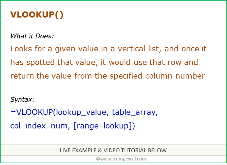
Use the VLOOKUP function to look up a value in a table.
Syntax
VLOOKUP (lookup_value, table_array, col_index_num, [range_lookup])
For example:
-
=VLOOKUP(A2,A10:C20,2,TRUE)
-
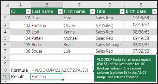
=VLOOKUP(«Fontana»,B2:E7,2,FALSE)
-
=VLOOKUP(A2,’Client Details’!A:F,3,FALSE)
|
Argument name |
Description |
|---|---|
|
lookup_value (required) |
The value you want to look up. The value you want to look up must be in the first column of the range of cells you specify in the table_array argument. For example, if table-array spans cells B2:D7, then your lookup_value must be in column B.
|
|
table_array (required) |
The range of cells in which the VLOOKUP will search for the lookup_value and the return value. You can use a named range or a table, and you can use names in the argument instead of cell references. The first column in the cell range must contain the lookup_value. The cell range also needs to include the return value you want to find. Learn how to select ranges in a worksheet. |
|
col_index_num (required) |
The column number (starting with 1 for the left-most column of table_array) that contains the return value. |
|
range_lookup (optional) |
A logical value that specifies whether you want VLOOKUP to find an approximate or an exact match:
|
How to get started
There are four pieces of information that you will need in order to build the VLOOKUP syntax:
-
The value you want to look up, also called the lookup value.
-
The range where the lookup value is located. Remember that the lookup value should always be in the first column in the range for VLOOKUP to work correctly. For example, if your lookup value is in cell C2 then your range should start with C.
-
The column number in the range that contains the return value. For example, if you specify B2:D11 as the range, you should count B as the first column, C as the second, and so on.
-
Optionally, you can specify TRUE if you want an approximate match or FALSE if you want an exact match of the return value. If you don’t specify anything, the default value will always be TRUE or approximate match.
Now put all of the above together as follows:
=VLOOKUP(lookup value, range containing the lookup value, the column number in the range containing the return value, Approximate match (TRUE) or Exact match (FALSE)).
Examples
Here are a few examples of VLOOKUP:
Example 1

Example 2
Example 3
Example 4
Example 5
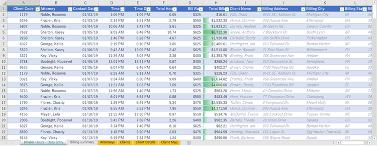
You can use VLOOKUP to combine multiple tables into one, as long as one of the tables has fields in common with all the others. This can be especially useful if you need to share a workbook with people who have older versions of Excel that don’t support data features with multiple tables as data sources — by combining the sources into one table and changing the data feature’s data source to the new table, the data feature can be used in older Excel versions (provided the data feature itself is supported by the older version).
|
|
Here, columns A-F and H have values or formulas that only use values on the worksheet, and the rest of the columns use VLOOKUP and the values of column A (Client Code) and column B (Attorney) to get data from other tables. |
-
Copy the table that has the common fields onto a new worksheet, and give it a name.
-
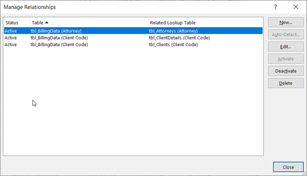
Click Data > Data Tools > Relationships to open the Manage Relationships dialog box.

-
For each listed relationship, note the following:
-
The field that links the tables (listed in parentheses in the dialog box). This is the lookup_value for your VLOOKUP formula.
-
The Related Lookup Table name. This is the table_array in your VLOOKUP formula.
-
The field (column) in the Related Lookup Table that has the data you want in your new column. This information is not shown in the Manage Relationships dialog — you’ll have to look at the Related Lookup Table to see which field you want to retrieve. You want to note the column number (A=1) — this is the col_index_num in your formula.
-
-
To add a field to the new table, enter your VLOOKUP formula in the first empty column using the information you gathered in step 3.
In our example, column G uses Attorney (the lookup_value) to get the Bill Rate data from the fourth column (col_index_num = 4) from the Attorneys worksheet table, tblAttorneys (the table_array), with the formula =VLOOKUP([@Attorney],tbl_Attorneys,4,FALSE).
The formula could also use a cell reference and a range reference. In our example, it would be =VLOOKUP(A2,’Attorneys’!A:D,4,FALSE).
-
Continue adding fields until you have all the fields that you need. If you are trying to prepare a workbook containing data features that use multiple tables, change the data source of the data feature to the new table.
|
Problem |
What went wrong |
|---|---|
|
Wrong value returned |
If range_lookup is TRUE or left out, the first column needs to be sorted alphabetically or numerically. If the first column isn’t sorted, the return value might be something you don’t expect. Either sort the first column, or use FALSE for an exact match. |
|
#N/A in cell |
For more information on resolving #N/A errors in VLOOKUP, see How to correct a #N/A error in the VLOOKUP function. |
|
#REF! in cell |
If col_index_num is greater than the number of columns in table-array, you’ll get the #REF! error value. For more information on resolving #REF! errors in VLOOKUP, see How to correct a #REF! error. |
|
#VALUE! in cell |
If the table_array is less than 1, you’ll get the #VALUE! error value. For more information on resolving #VALUE! errors in VLOOKUP, see How to correct a #VALUE! error in the VLOOKUP function. |
|
#NAME? in cell |
The #NAME? error value usually means that the formula is missing quotes. To look up a person’s name, make sure you use quotes around the name in the formula. For example, enter the name as «Fontana» in =VLOOKUP(«Fontana»,B2:E7,2,FALSE). For more information, see How to correct a #NAME! error. |
|
#SPILL! in cell |
This particular #SPILL! error usually means that your formula is relying on implicit intersection for the lookup value, and using an entire column as a reference. For example, =VLOOKUP(A:A,A:C,2,FALSE). You can resolve the issue by anchoring the lookup reference with the @ operator like this: =VLOOKUP(@A:A,A:C,2,FALSE). Alternatively, you can use the traditional VLOOKUP method and refer to a single cell instead of an entire column: =VLOOKUP(A2,A:C,2,FALSE). |
|
Do this |
Why |
|---|---|
|
Use absolute references for range_lookup |
Using absolute references allows you to fill-down a formula so that it always looks at the same exact lookup range. Learn how to use absolute cell references. |
|
Don’t store number or date values as text. |
When searching number or date values, be sure the data in the first column of table_array isn’t stored as text values. Otherwise, VLOOKUP might return an incorrect or unexpected value. |
|
Sort the first column |
Sort the first column of the table_array before using VLOOKUP when range_lookup is TRUE. |
|
Use wildcard characters |
If range_lookup is FALSE and lookup_value is text, you can use the wildcard characters—the question mark (?) and asterisk (*)—in lookup_value. A question mark matches any single character. An asterisk matches any sequence of characters. If you want to find an actual question mark or asterisk, type a tilde (~) in front of the character. For example, =VLOOKUP(«Fontan?»,B2:E7,2,FALSE) will search for all instances of Fontana with a last letter that could vary. |
|
Make sure your data doesn’t contain erroneous characters. |
When searching text values in the first column, make sure the data in the first column doesn’t have leading spaces, trailing spaces, inconsistent use of straight ( ‘ or » ) and curly ( ‘ or “) quotation marks, or nonprinting characters. In these cases, VLOOKUP might return an unexpected value. To get accurate results, try using the CLEAN function or the TRIM function to remove trailing spaces after table values in a cell. |
Need more help?
You can always ask an expert in the Excel Tech Community or get support in the Answers community.

See Also
XLOOKUP function
Video: When and how to use VLOOKUP
Quick Reference Card: VLOOKUP refresher
How to correct a #N/A error in the VLOOKUP function
Look up values with VLOOKUP, INDEX, or MATCH
HLOOKUP function
Need more help?
VLOOKUP is an Excel function to get data from a table organized vertically. Lookup values must appear in the first column of the table passed into VLOOKUP. VLOOKUP supports approximate and exact matching, and wildcards (* ?) for partial matches.
Vertical data | Column Numbers | Only looks right | Matching Modes | Exact Match | Approximate Match | First Match | Wildcard Match | Two-way Lookup | Multiple Criteria | #N/A Errors | Videos
Introduction
VLOOKUP is probably the most famous function in Excel, for reasons both good and bad. On the good side, VLOOKUP is easy to use and does something very useful. For new users in particular, it is immensely satisfying to watch VLOOKUP scan a table, find a match, and return a correct result. Using VLOOKUP successfully is a rite of passage for new Excel users.
On the bad side, VLOOKUP is limited and has dangerous defaults. Unlike INDEX and MATCH (or XLOOKUP), VLOOKUP needs a complete table with lookup values in the first column. This makes it hard to use VLOOKUP with multiple criteria. In addition, VLOOKUP’s default matching behavior makes it easy to get incorrect results. Fear not. The key to using VLOOKUP successfully is mastering the basics. Read on for a complete overview.
Arguments
VLOOKUP takes four arguments: lookup_value, table_array, column_index_num, and range_lookup. Lookup_value is the value to look for, and table_array is the range of vertical data to look inside. The first column of table_array must contain the lookup values to search. The column_index_num argument is the column number of the value to retrieve, where the first column of table_array is column 1. Finally, range_lookup controls match behavior. If range_lookup is TRUE, VLOOKUP will perform an approximate match. If range_lookup is FALSE, VLOOKUP will perform an exact match. Important: range_lookup is optional and defaults to TRUE, so VLOOKUP will perform an approximate match by default. See below for more information on matching.
V is for vertical
The purpose of VLOOKUP is to look up information in a table like this:

With the Order number in column B as the lookup_value, VLOOKUP can get the Cust. ID, Amount, Name, and State for any order. For example, to get the name for order 1004, the formula is:
=VLOOKUP(1004,B5:F9,4,FALSE) // returns "Sue Martin"
To look up horizontal data, you can use HLOOKUP, INDEX and MATCH, or XLOOKUP.
VLOOKUP is based on column numbers
When you use VLOOKUP, imagine that every column in the table_array is numbered, starting from the left. To get a value from a given column, provide the number for column_index_num. For example, the column index to retrieve the first name below is 2:

By changing only column_index_num, you can look up columns 2, 3, and 4:
=VLOOKUP(H3,B4:E13,2,FALSE) // first name
=VLOOKUP(H3,B4:E13,3,FALSE) // last name
=VLOOKUP(H3,B4:E13,4,FALSE) // email address
Note: normally, we would use an absolute reference for H3 ($H$3) and B4:E13 ($B$4:$E$13) to prevent these from changing when the formula is copied. Above, the references are relative to make them easier to read.
VLOOKUP only looks right
VLOOKUP can only look to the right. In other words, you can only retrieve data to the right of the column that holds lookup values:

To look up values to the left, see INDEX and MATCH, or XLOOKUP.
Match modes
VLOOKUP has two modes of matching, exact and approximate, controlled by the fourth argument, range_lookup. The word «range» in this case refers to «range of values» – when range_lookup is TRUE, VLOOKUP will match a range of values rather than an exact value. A good example of this is using VLOOKUP to calculate grades. When range_lookup is FALSE, VLOOKUP performs an exact match, as in the example above.
Important: range_lookup is optional defaults to TRUE. This means approximate match mode is the default, which can be dangerous. Set range_lookup to FALSE to force exact matching:
=VLOOKUP(value,table,col_index) // approximate match (default)
=VLOOKUP(value,table,col_index,TRUE) // approximate match
=VLOOKUP(value,table,col_index,FALSE) // exact match
Tip: always supply a value for range_lookup as a reminder of expected behavior.
Note: You can also supply zero (0) for an exact match, and 1 for an approximate match.
Exact match example
In most cases, you’ll probably want to use VLOOKUP in exact match mode. This makes sense when you have a unique key to use as a lookup value, for example, the movie title in this data:

The formula in H6 to find Year, based on an exact match of the movie title, is:
=VLOOKUP(H4,B5:E9,2,FALSE) // FALSE = exact match
Approximate match example
In some cases, you will need an approximate match lookup instead of an exact match lookup. For example, below we want to find the correct commission percentage in the range G5:H10 based on the sales amount in column C. In this example, we need to use VLOOKUP in approximate match mode, because in most cases an exact match will never be found. The VLOOKUP formula in D5 is configured to perform an approximate match by setting the last argument to TRUE:

=VLOOKUP(C5,$G$5:$H$10,2,TRUE) // TRUE = approximate match
VLOOKUP will scan values in column G for the lookup value. If an exact match is found, VLOOKUP will use it. If not, VLOOKUP will «step back» and match the previous row.
Note: The table_array must be sorted in ascending order by lookup value to use an approximate match. If table_array is not sorted by the first column in ascending order, VLOOKUP may return incorrect or unexpected results.
First match only
In the case of duplicate matching values, VLOOKUP will find the first match. In the screen below, VLOOKUP is configured to find the price for the color «Green». There are three rows with the color Green, and VLOOKUP returns the price in the first row, $17. The formula in cell F5 is:
=VLOOKUP(E5,B5:C11,2,FALSE) // returns 17

Tip: To retrieve multiple matches with a lookup operation, see the FILTER function.
Wildcard match
The VLOOKUP function supports wildcards, which makes it possible to perform a partial match on a lookup value. For instance, you can use VLOOKUP to retrieve information from a table with a partial lookup_value and wildcard. To use wildcards with VLOOKUP, you must use exact match mode by providing FALSE for range_lookup. In the screen below, the formula in H7 retrieves the first name, «Michael», after typing «Aya» into cell H4. Notice the asterisk (*) wildcard is concatenated to the lookup value inside the VLOOKUP formula:
=VLOOKUP($H$4&"*",$B$5:$E$104,2,FALSE)

Read a more detailed explanation here.
Two-way lookup
Inside the VLOOKUP function, column_index_num is normally hard-coded as a static number. However, you can create a dynamic column index by using the MATCH function to locate the needed column. This technique allows you to create a dynamic two-way lookup, matching on both rows and columns. In the screen below, VLOOKUP is configured to perform a lookup based on Name and Month like this:
=VLOOKUP(H4,B5:E13,MATCH(H5,B4:E4,0),0)

For more details, see this example.
Note: In general, INDEX and MATCH is a more flexible way to perform two-way lookups.
Multiple criteria
The VLOOKUP function does not handle multiple criteria natively. However, you can use a helper column to join multiple fields together and use these fields like multiple criteria inside VLOOKUP. In the example below, Column B is a helper column that concatenates first and last names together with this formula:
=C5&D5 // helper column
VLOOKUP is configured to do the same thing to create a lookup value. The formula in H6 is:
=VLOOKUP(H4&H5,B5:E13,4,0)

For details, see this example. For a more advanced, flexible approach, see this example.
Note: INDEX and MATCH and XLOOKUP are better for lookups based on multiple criteria.
VLOOKUP and #N/A errors
If you use VLOOKUP you will inevitably run into the #N/A error. The #N/A error means «not found». For example, in the screen below, the lookup value «Toy Story 2» does not exist in the lookup table, and all three VLOOKUP formulas return #N/A:

The #N/A error is useful because tells you something is wrong. The reason for #N/A might be:
- The lookup value does not exist in the table
- The lookup value is misspelled or contains extra space
- Match mode is exact, but should be approximate
- The table range is not entered correctly
- You are copying VLOOKUP, and the table reference is not locked
To «trap» the NA error and return a different value, you can use the IFNA function like this:

The formula in H6 is:
=IFNA(VLOOKUP(H4,B5:E9,2,FALSE),"Not found")
The message can be customized as desired. To return nothing (i.e. to display a blank result) when VLOOKUP returns #N/A you can use an empty string («») like this:
=IFNA(VLOOKUP(H4,B5:E9,2,FALSE),"") // no message
You can also use the IFERROR function to trap VLOOKUP #N/A errors. However, be careful with IFERROR, because it will catch any error, not just the #N/A error. Read more: VLOOKUP without #N/A errors
More about VLOOKUP
- VLOOKUP with multiple criteria (basic)
- VLOOKUP with multiple criteria (advanced)
- How to use VLOOKUP to merge tables
- 23 tips for using VLOOKUP
- More VLOOKUP examples and videos
- XLOOKUP vs VLOOKUP
Other notes
- VLOOKUP performs an approximate match by default.
- VLOOKUP is not case-sensitive.
- Range_lookup controls the match mode. FALSE = exact, TRUE = approximate (default).
- If range_lookup is omitted or TRUE or 1:
- VLOOKUP will match the nearest value less than the lookup_value.
- VLOOKUP will still use an exact match if one exists.
- The column 1 of table_array must be sorted in ascending order.
- If range_lookup is FALSE or zero:
- VLOOKUP performs an exact match.
- Column 1 of table_array does not need to be sorted.
The Function VLOOKUP in Excel allows rearranging data from one table to the corresponding cells in another one.
It’s very handy and frequently used. As it’s a problematic thing to compare manually ranges with tens of thousands of names.
How to use The Function VLOOKUP in Excel
For example, the warehouse of the enterprise for the production of packaging received materials in a certain amount. The cost of materials is in the price list. This is a separate table.
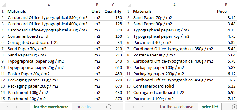
It is necessary to find out the cost of materials received at the warehouse. To do this we should substitute the price of the second table in the first. And by ordinary multiplication we will find the title.
Algorithm:
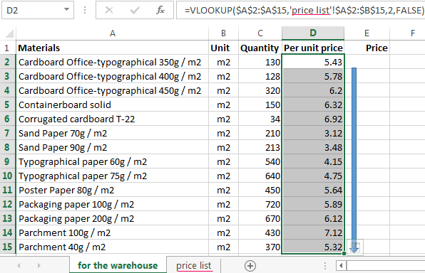
- Here is the first table (for the warehouse) in the required view. Add columns «Per unit price» and total «Price». Establish a currency format for the new cells.
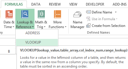
- Select the first cell in the «Price» column. In our example it’s D2. Call the «Insert Function» using the «FX» button (at the beginning of the formula bar) or by pressing the hot key combination SHIFT + F3. In the category «Lookup & Reference» we find the function =VLOOKUP(), and click OK. This function can be called up by clicking on the «FORMULAS» tab and choose from the drop-down list of «Lookup & Reference».
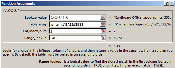
- A window with the function arguments will be opened. In the field «Lookup_value» — the first column of the range of data from the table with the number of received materials. These are the values that Excel should find in the second table.
- The next argument is «Table_array». This is our price list. Put the cursor in the field of argument than go to the list prices. Select the range with the names of materials and prices. Show what value the function should match.
- For Excel to refer directly to these data, it is necessary to fix the link. Select «Table_array» field value and press F4. $ Icon appears.
- In the argument «Col_index_num» put the number «2». Here are the data that you need to get in the first table. «Range_lookup» is FALSE. As we need specific, not approximate.
Click OK. And then copy the function of that column: we catch a mouse bottom right corner and drag down. We get the necessary result.
Now to find the cost of materials is not difficult: the number of * cost.
Function VLOOKUP linked the two tables. If you change the price, and then change the value of the materials received at the warehouse (now received). To avoid this, use the «Paste Special».
- Select the column with inserted prices.
- Use the right mouse button – «Copy».
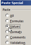
- Still selected use the right mouse button – «Paste Special».
- Put a tick next to «Values». OK.
The formulas in the cells disappear. Only values remain.
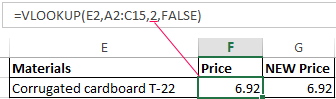
A quick comparison of the two tables with the help of VLOOKUP
The function helps to compare the values in large tables. In case of the price has changed. We need to compare the old prices with the new prices.
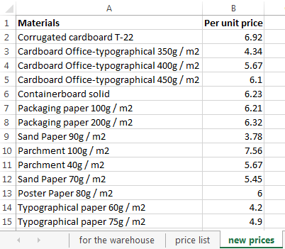
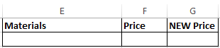
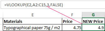
- In the old price list do the column «NEW Price».
- Select the first cell and select the function VLOOKUP. The given examples (see. Above). For example:

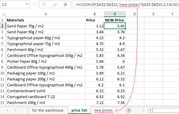
This means that you need to take the name of the material from the range A2: A15, look it up in the «new prices» in column A. Then take the data from the second column of the new price (Per unit price) and substitute them in cell C2 under «NEW Price».
The data presented in this way, can be compared. We can find the numeral and percentage difference.
The function VLOOKUP in Excel with multiple conditions
Until now, we have offered for the analysis of only one condition — the name of the material. In practice, it often requires several bands to compare and select the data value 2, 3 and other criteria.
Table for example:
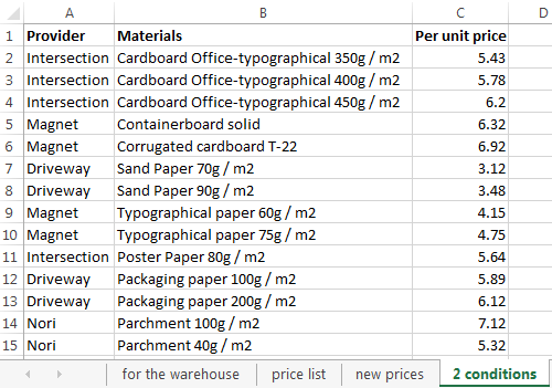
Guessing we need to find, what is the price of the corrugated cardboard of JSC «Magnet». It is necessary to set two conditions to search the name of the material and the vendor.
The matter is complicated by the fact that one supplier receives several names.
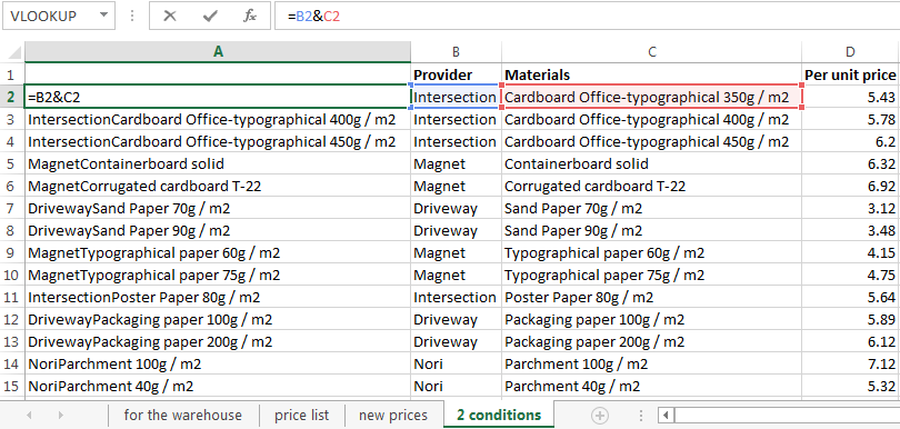
- Adding to the table the leftmost column (important!), combining the «Provider» and «Materials».
- We combine the required criteria the same way:
- Put the cursor in the right place H3 and set arguments for function:
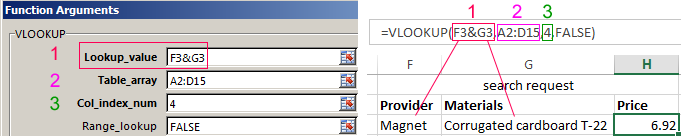
Excel finds the right price.
Consider the formula in detail:
- What we are looking for – request the addition of a criterion F3&G3.
- Where to look for – range of data A2:D15.
- What data to take – column number 4 in the range A2:D15.
The Function VLOOKUP and drop-down list
For example, some data is made in the form of a drop-down list. In our example it is «Materials». It is necessary to configure the function so that when choosing names appeared prices.
First do drop-down list:
- Go to sheet «price list» and create a table for requests in the range E1:G2.
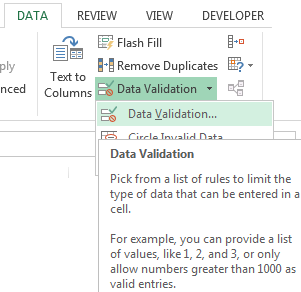
- Put the cursor in cell F3, where will be this list and go to the tab «DATA». «Data Validation» menu.
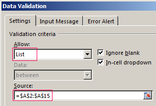
- Select the type of data – «List». Source is the range with the names of materials.
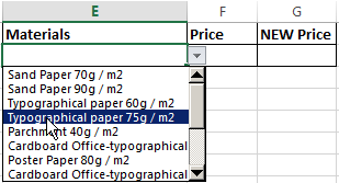
- When press the OK the dropdown list is formed.
Now you need to make the way when choosing a particular material in the column price corresponding figure appeared. Put the cursor in the F2 cell (which will have to appear the price).
- Open the window «Insert Function» and select VLOOKUP.
- The first argument is «Lookup_value» – the box with drop-down list. The table is a range of materials with names and prices. And column 2. Function has acquired the following form:
- In a cell G2, enter the formula (formula different column number 3):
- Press ENTER and enjoy the result.
Change the material — the price changes:
Download this example VLOOKUP in Excel
This is how the drop down list in Excel with the function of the VLOOKUP. Everything happens automatically within a few seconds. Everything works quickly and accurately. It is necessary to deal with this function.
VLOOKUP Function – Introduction
VLOOKUP function is THE benchmark.
You know something in Excel if you know how to use the VLOOKUP function.
If you don’t, you better not list Excel as one of your strong areas in your resume.
I have been a part of the panel interviews where as soon as the candidate mentioned Excel as his area of expertise, the first thing asked was – you got it – the VLOOKUP function.
Now that we know how important this Excel function is, it makes sense to ace it completely to be able to proudly say – “I know a thing or two in Excel”.
This is going to be a massive VLOOKUP tutorial (by my standards).
I’ll cover everything there is to know about it, and then show you useful and practical VLOOKUP examples.
So buckle up.
It’s time for the takeoff.
When to use the VLOOKUP Function in Excel?
VLOOKUP function is best suited for situations when you are looking for a matching data point in a column, and when the matching data point is found, you go to the right in that row and fetch a value from a cell which is a specified number of columns to the right.
Let’s take a simple example here to understand when to use Vlookup in Excel.
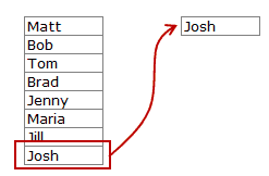
Remember when the exam score list was out and pasted on the notice board and everyone used to go crazy finding their names and their score (at least that’s what used to happen when I was in school).
Here is how it worked:
- You go up to the notice board and start looking for your name or enrolment number (running your finger from top to bottom in the list).
- As soon as you spot your name, you move your eyes to the right of the name/enrolment number to see your scores.
And that is exactly what the Excel VLOOKUP function does for you (feel free to use this example in your next interview).
VLOOKUP function looks for a specified value in a column (in the above example, it was your name) and when it finds the specified match, it returns a value in the same row (the marks you obtained).
Syntax
=VLOOKUP(lookup_value, table_array, col_index_num, [range_lookup])
Input Arguments
- lookup_value – this is the look-up value you are trying to find in the left-most column of a table. It could be a value, a cell reference, or a text string. In the score sheet example, this would be your name.
- table_array – this is the table array in which you are looking for the value. This could be a reference to a range of cells or a named range. In the score sheet example, this would be the entire table that contains score for everyone for every subject
- col_index – this is the column index number from which you want to fetch the matching value. In the score sheet example, if you want the scores for Math (which is the first column in a table that contains the scores), you’d look in column 1. If you want the scores for Physics, you’d look in column 2.
- [range_lookup] – here you specify whether you want an exact match or an approximate match. If omitted, it defaults to TRUE – approximate match (see additional notes below).
Additional Notes (Boring, but important to know)
- The match could be exact (FALSE or 0 in range_lookup) or approximate (TRUE or 1).
- In approximate lookup, make sure that the list is sorted in ascending order (top to bottom), or else the result could be inaccurate.
- When range_lookup is TRUE (approximate lookup) and data is sorted in ascending order:
- If the VLOOKUP function can not find the value, it returns the largest value, which is less than the lookup_value.
- It returns a #N/A error if the lookup_value is smaller than the smallest value.
- If lookup_value is text, wildcard characters can be used (refer to the example below).
Now, hoping that you have a basic understanding of what the VLOOKUP function can do, let’s peel this onion and see some practical examples of the VLOOKUP function.
10 Excel VLOOKUP Examples (Basic & Advanced)
Here are 10 useful exampels of using Excel Vlookup that will show you how to use it in your day-to-day work.
Example 1 – Finding Brad’s Math Score
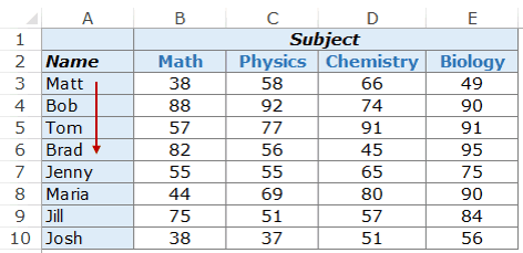
In the VLOOKUP example below, I have a list wth student names in the left-most column and marks in different subjects in columns B to E.
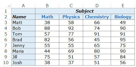
Now let’s get to work and use the VLOOKUP function for what it does best. From the above data, I need to know how much Brad scored in Math.
From the above data, I need to know how much Brad scored in Math.
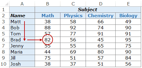
Here is the VLOOKUP formula that will return Brad’s Math score:
=VLOOKUP("Brad",$A$3:$E$10,2,0)
The above formula has four arguments:
- “Brad: – this is the lookup value.
- $A$3:$E$10 – this is the range of cells in which we are looking. Remember that Excel looks for the lookup value in the left-most column. In this example, it would look for the name Brad in A3:A10 (which is the left-most column of the specified array).
- 2 – Once the function spots Brad’s name, it will go to the second column of the array, and return the value in the same row as that of Brad. The value 2 here indicated that we are looking for the score from the second column of the specified array.
- 0 – this tells the VLOOKUP function to only look for exact matches.
Here is how the VLOOKUP formula works in the above example.
First, it looks for the value Brad in the left-most column. It goes from top to bottom and finds the value in cell A6.
As soon as it finds the value, it goes to the right in the second column and fetches the value in it.
You can use the same formula construct to get anyone’s marks in any of the subjects.
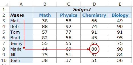
For example, to find Maria’s marks in Chemistry, use the following VLOOKUP formula:
=VLOOKUP("Maria",$A$3:$E$10,4,0)
In the above example, the lookup value (student’s name) is entered in double quotes. You can also use a cell reference that contains the lookup value.
The benefit of using a cell reference is that it makes the formula dynamic.
For example, if you have a cell with a student’s name, and you are fetching the score for Math, the result would automatically update when you change the student’s name (as shown below):
If you enter a lookup value that is not found in the left-most column, it returns a #N/A error.
Example 2 – Two-Way Lookup
In Example 1 above, we hard-coded the column value. Hence, the formula would always return the score for Math as we have used 2 as the column index number.
But what if you want to make both the VLOOKUP value and the column index number dynamic. For example, as shown below, you can change either the student name or the subject name, and the VLOOKUP formula fetches the correct score. This is an example of a two-way VLOOKUP formula.
This is an example of a two-way VLOOKUP function.
To make this two-way lookup formula, you need to make the column dynamic as well. So when a user changes the subject, the formula automatically picks the correct column (2 in the case of Math, 3 in the case of Physics, as so on..).
To do this, you need to use the MATCH function as the column argument.
Here is the VLOOKUP formula that will do this:
=VLOOKUP(G4,$A$3:$E$10,MATCH(H3,$A$2:$E$2,0),0)
The above formula uses MATCH(H3,$A$2:$E$2,0) as the column number. MATCH function takes the subject name as the lookup value (in H3) and returns its position in A2:E2. Hence, if you use Math, it would return 2 as Math is found in B2 (which is the second cell in the specified array range).
Example 3 – Using Drop Down Lists as Lookup Values
In the above example, we have to manually enter the data. That could be time-consuming and error-prone, especially if you have a huge list of lookup values.
A good idea in such cases is to create a drop-down list of the lookup values (in this case, it could be student names and subjects) and then simply choose from the list.
Based on the selection, the formula would automatically update the result.
Something as shown below:
This makes a good dashboard component as you can have a huge data set with hundreds of students at the back end, but the end user (let’s say a teacher) can quickly get the marks of a student in a subject by simply making the selections from the drop down.
How to make this:
The VLOOKUP formula used in this case is the same used in Example 2.
=VLOOKUP(G4,$A$3:$E$10,MATCH(H3,$A$2:$E$2,0),0)
The lookup values have been converted into drop-down lists.
Here are the steps to create the drop down list:
- Select the cell in which you want the drop-down list. In this example, in G4, we want the student names.
- Go to Data –> Data Tools –> Data Validation.
- In the Data Validation Dialogue box, within the settings tab, select List from the Allow drop-down.
- In the source, select $A$3:$A$10
- Click OK.
Now you’ll have the drop-down list in cell G4. Similarly, you can create one in H3 for the subjects.
Example 4 – Three-way Lookup
What is a three-way lookup?
In Example 2, we’ve used one lookup table with scores for students in different subjects. This is an example of a two-way lookup as we use two variables to fetch the score (student’s name and the subject’s name).
Now, suppose in a year, a student has three different levels of exams, Unit Test, Midterm, and Final Examination (that’s what I had when I was a student).
A three-way lookup would be the ability to get a student’s marks for a specified subject from the specified level of exam.
Something as shown below:
In the above example, the VLOOKUP function can lookup in three different tables (Unit Test, Midterm, and Final Exam) and returns the score for the specified student in the specified subject.
Here is the formula used in cell H4:
=VLOOKUP(G4,CHOOSE(IF(H2="Unit Test",1,IF(H2="Midterm",2,3)),$A$3:$E$7,$A$11:$E$15,$A$19:$E$23),MATCH(H3,$A$2:$E$2,0),0)
This formula uses the CHOOSE function to make sure the right table is referred to. Let’s analyze the CHOOSE part of the formula:
CHOOSE(IF(H2=”Unit Test”,1,IF(H2=”Midterm”,2,3)),$A$3:$E$7,$A$11:$E$15,$A$19:$E$23)
The first argument of the formula is IF(H2=”Unit Test”,1,IF(H2=”Midterm”,2,3)), which checks the cell H2 and see what level of exam is being referred to. If it’s Unit Test, it returns $A$3:$E$7, which has the scores for Unit Test. If it’s Midterm, it returns $A$11:$E$15, else it returns $A$19:$E$23.
Doing this makes the VLOOKUP table array dynamic and hence makes it a three-way lookup.
Example 5 – Getting the Last Value from a List
You can create a VLOOKUP formula to get the last numerical value from a list.
The largest positive number that you can use in Excel is 9.99999999999999E+307. This also means that the largest lookup number in the VLOOKUP number is also the same.
I don’t think you would ever need any calculation involving such a large number. And that is exactly what we can use get the last number in a list.
Suppose you have a dataset (in A1:A14) as shown below and you want to get the last number in the list.
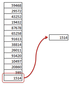
Here is the formula you can use:
=VLOOKUP(9.99999999999999E+307,$A$1:$A$14,TRUE)
Note that the formula above uses an approximate match VLOOKUP (notice TRUE at the end of the formula, instead of FALSE or 0). Also, note that the list doesn’t need to be sorted for this VLOOKUP formula to work.
Here is how the approximate VLOOKUP function works. It scans the left most column from top to bottom.
- If it finds an exact match, it returns that value.
- If it finds a value that is higher than the lookup value, it returns the value in the cell above it.
- If the lookup value is greater than all the values in the list, it returns the last value.
In the above example, the third scenario is at work.
Since 9.99999999999999E+307 is the largest number that can be used in Excel, when this is used as the lookup value, it returns the last number from the list.
In the same way, you can also use it to return the last text item from the list. Here is the formula that can do that:
=VLOOKUP("zzz",$A$1:$A$8,1,TRUE)
The same logic follows. Excel looks through all the names, and since zzz is considered bigger than any name/text starting with alphabets before zzz, it would return the last item from the list.
Example 6 – Partial Lookup using Wildcard Characters and VLOOKUP
Excel wildcard characters can be really helpful in many situations.
It’s that magic potion that gives your formulas super powers.
Partial look-up is needed when you have to look for a value in a list and there isn’t an exact match.
For example, suppose you have a data set as shown below, and you want to look for the company ABC in a list, but the list has ABC Ltd instead of ABC.
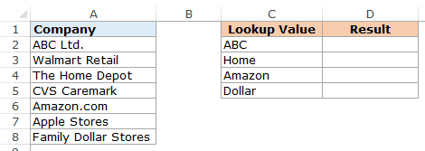
You can not use ABC as the lookup value as there is no exact match in column A. Approximate match also leads to erroneous results and it requires the list to be sorted in an ascending order.
However, you can use a wildcard character within the VLOOKUP function to get the match.
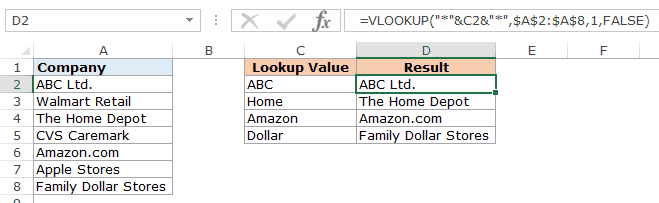
Enter the following formula in cell D2 and drag it to the other cells:
=VLOOKUP("*"&C2&"*",$A$2:$A$8,1,FALSE)
How does this formula work?
In the above formula, instead of using the lookup value as is, it is flanked on both sides with the wildcard character asterisk (*) – “*”&C2&”*”
An asterisk is a wildcard character in Excel and can represent any number of characters.
Using the asterisk on both sides of the lookup value tells Excel that it needs to look for any text that contains the word in C2. It could have any number of characters before or after the text in C2.
For example, cell C2 has ABC, so the VLOOKUP function looks through the names in A2:A8 and searches for ABC. It finds a match in cell A2, as it contains ABC in ABC Ltd. It doesn’t matter if there are any characters to the left or right of ABC. Until there is ABC in a text string, it will be considered a match.
Note: VLOOKUP function always returns the first matching value and stops looking further. So if you have ABC Ltd., and ABC Corporation in a list, it will return the first one and ignore the rest.
Example 7 – VLOOKUP Returning an Error Despite a Match in Lookup Value
It can drive you crazy when you see that there is a matching lookup value and the VLOOKUP function is returning an error.
For example, in the below case, there is a match (Matt), but the VLOOKUP function still returns an error.
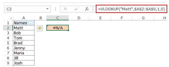
Now while we can see there is a match, what we can not see with a naked eye is that there could be leading or trailing spaces. If you have these additional spaces before, after, or in between the lookup values, it ISN’T an exact match.
This is often the case when you import data from a database or get it from someone else. These leading/trailing spaces have a tendency to sneak in.
The solution here is the TRIM function. It removes any leading or trailing spaces or extra spaces between words.
Here is the formula that’ll give you the right result.
=VLOOKUP("Matt",TRIM($A$2:$A$9),1,0)
Since this is an array formula, use Control + Shift + Enter instead of just Enter.
Another way could be to first treat your lookup array with the TRIM function to make sure all the additional spaces are gone, and then use the VLOOKUP function as usual.
Example 8 – Doing a Case Sensitive Lookup
By default, the lookup value in the VLOOKUP function is not case sensitive. For example, if your lookup value is MATT, matt, or Matt, it’s all the same for the VLOOKUP function. It’ll return the first matching value irrespective of the case.
But if you want to do a case-sensitive lookup, you need to use the EXACT function along with the VLOOKUP function.
Here is an example:
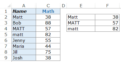
As you can see, there are three cells with the same name (in A2, A4, and A5) but with a different alphabet case. On the right, we have the three names (Matt, MATT, and matt) along with their scores in Math.
Now the VLOOKUP function is not equipped to handle case-sensitive lookup values. In this above example, it would always return 38, which is the score for Matt in A2.
To make it case sensitive, we need to use a helper column (as shown below):
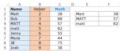
To get the values in the helper column, use the =ROW() function. It will simply get the row number in the cell.
Once you have the helper column, here is the formula that will give the case-sensitive lookup result.
=VLOOKUP(MAX(EXACT(E2,$A$2:$A$9)*(ROW($A$2:$A$9))),$B$2:$C$9,2,0)
Now let’s break down and understand what this does:
- EXACT(E2,$A$2:$A$9) – This part would compare the lookup value in E2 with all the values in A2:A9. It returns an array of TRUEs/FALSEs where TRUE is returned where there is an exact match. In this case, it would return the following array: {TRUE;FALSE;FALSE;FALSE;FALSE;FALSE;FALSE;FALSE}.
- EXACT(E2,$A$2:$A$9)*(ROW($A$2:$A$9) – This part multiplies the array of TRUEs/FALSEs with the row number. Wherever there is a TRUE, it gives the row number, else it gives 0. In this case, it would return {2;0;0;0;0;0;0;0}.
- MAX(EXACT(E2,$A$2:$A$9)*(ROW($A$2:$A$9))) – This part returns the maximum value from the array of numbers. In this case, it would return 2 (which is the row number where there is an exact match).
- Now we simply use this number as the lookup value and use the lookup array as B2:C9
Note: Since this is an array formula, use Control + Shift + Enter instead of just enter.
Example 9 – Using VLOOKUP with Multiple Criteria
Excel VLOOKUP function, in its basic form, can look for one lookup value and return the corresponding value from the specified row.
But often there is a need to use VLOOKUP in Excel with multiple criteria.
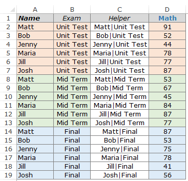
Suppose you have a data with students name, exam type, and the Math score (as shown below):
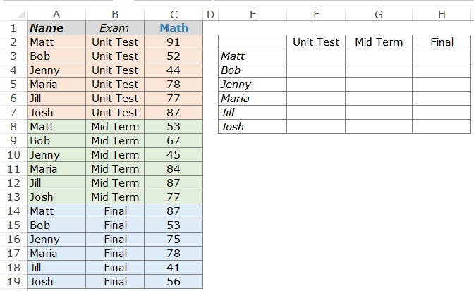
Using the VLOOKUP function to get the Math score for each student for respective exam levels could be a challenge.
For example, if you try using VLOOKUP with Matt as the lookup value, it’ll always return 91, which is the score for the first occurrence of Matt in the list. To get the score for Matt for each exam type (Unit Test, Mid Term and Final), you need to create a unique lookup value.
This can be done using the helper column. The first step is to insert a helper column to the left of the scores.
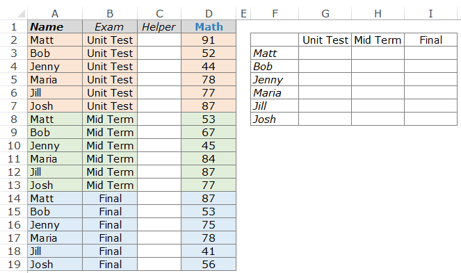
Now, to create a unique qualifier for each instance of the name, use the following formula in C2: =A2&”|”&B2
Copy this formula to all the cells in the helper column. This will create unique lookup values for each instance of a name (as shown below):
Now, while there were repetitions of the names, there is no repetition when the name is combined with the level of examination.
This makes it easy as now you can use the helper column values as the lookup values.
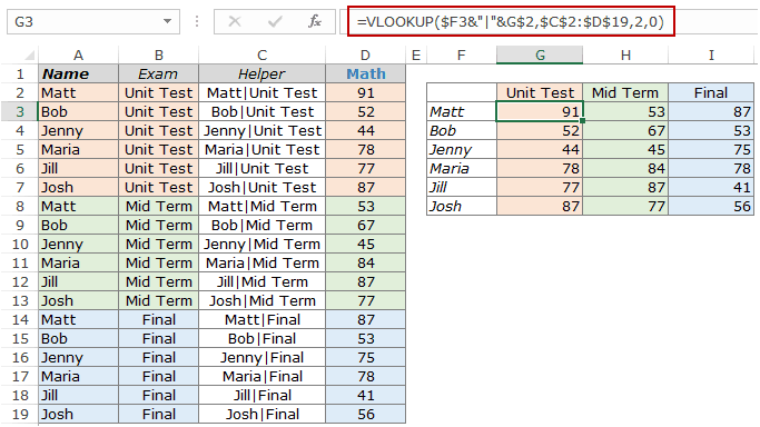
Here is the formula that’ll give you the result in G3:I8.
=VLOOKUP($F3&"|"&G$2,$C$2:$D$19,2,0)
Here we have combined the student name and the level of examination to get the lookup value, and we use this lookup value and checks it in the helper column to get the matching record.
Note: In the above example, we have used | as the separator while joining text in the helper column. In some exceptionally rare (but possible) conditions, you may have two criteria that are different but ends up giving the same result when combined. Here is an example:
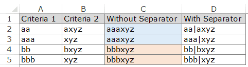
Note that while A2 and A3 are different and B2 and B3 are different, the combinations end up being the same. But if you use a separator, then even the combination would be different (D2 and D3).
Here is a tutorial on how to use VLOOKUP with multiple criteria without using helper columns. You can also watch my video tutorial here.
Example 10 – Handling Errors while Using the VLOOKUP Function
Excel VLOOKUP function returns an error when it can not find the specified lookup value. You may not want the ugly error value disturbing the aesthetics of your data in case VLOOKUP can’t find a value.
You can easily remove the error values with any meaning full text such as “Not Available” or “Not Found”.
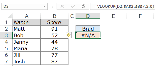
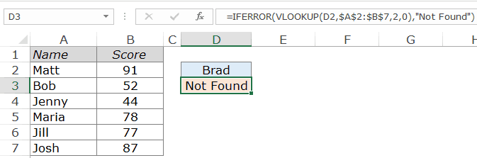
For example, in the example below, when you try to find the score of Brad in the list, it returns an error as Brad’s name is not there in the list.
To remove this error and replace it with something meaningful, wrap your VLOOKUP function within the IFERROR function.
Here is the formula:
=IFERROR(VLOOKUP(D2,$A$2:$B$7,2,0),"Not Found")
The IFERROR function checks if the value returned by the first argument (which is the VLOOKUP function in this case) is an error or not. If it’s not an error, it returns the value by the VLOOKUP function, else it returns Not Found.
IFERROR function is available from Excel 2007 onwards. If you are using versions prior to that, use the following function:
=IF(ISERROR(VLOOKUP(D2,$A$2:$B$7,2,0)),"Not Found",VLOOKUP(D2,$A$2:$B$7,2,0))
Also See: How to handle VLOOKUP Errors in Excel.
That’s it in this VLOOKUP tutorial.
I’ve tried to cover major examples of using the Vlookup function in Excel. If you would like to see more examples added to this list, let me know in the comments section.
Note: I’ve tried my best to proofread this tutorial, but in case you find any errors or spelling mistakes, please let me know 🙂
Using VLOOKUP Function in Excel – Video
Related Excel Functions:
- Excel HLOOKUP Function.
- Excel XLOOKUP Function
- Excel INDEX Function.
- Excel INDIRECT Function.
- Excel MATCH Function.
- Excel OFFSET Function.
You May Also Like the Following Excel Tutorials:
- VLOOKUP Vs. INDEX/MATCH – The Debate ends here.
- Excel Index Match Examples
- How to Make VLOOKUP Function Case Sensitive.
- Get Multiple Lookup Values Without Repetition in a Single Cell
- Avoid Nested IF Function in Excel by using VLOOKUP
The VLOOKUP Excel function searches for a particular value and returns a corresponding match based on a unique identifier. A unique identifier is uniquely associated with all the records of the database. For instance, employee ID, student roll number, customer contact number, seller email address, etc., are unique identifiers.
For example, suppose you have a dataset of employee salaries ($150, $200, $500, $800 from B2:B5 and employee ID (1001,1002,1003,1004) from A2:A5. Then, in cell E2, we want to know the employee ID for the salary of $200, which is in cell B3. In such a scenario, we can use the VLOOKUP function. Then, inserting the lookup_value in cell D2, we can enter the formula as:
= VLOOKUP(D2,A2:B5,2,FALSE). It returns “1002”
In simple words, a user may use the VLOOKUP formula to search specific information (like employee ID) in an Excel database (table in Excel worksheet) and find information associated (employee’s salary) with it.
The “V” in VLOOKUP stands for vertical. The function looks for a search value in the first column (lookup column) of the specified range and returns a match from the same row of another column (return column).
The VLOOKUP Excel function works for numerical, textual, and logical values. For example, an organization uses VLOOKUP to retrieve the monthly revenue of multiple products based on the product code (unique identifier).
Table of contents
- VLOOKUP Function
- The Syntax of the VLOOKUP Function
- How to Use VLOOKUP in Excel?
- Example #1
- Example #2
- Example #3
- The Characteristics of VLOOKUP Function
- The VLOOKUP Errors in Excel
- Frequently Asked Questions
- Recommended Articles
You are free to use this image on your website, templates, etc, Please provide us with an attribution linkArticle Link to be Hyperlinked
For eg:
Source: VLOOKUP Function in Excel (wallstreetmojo.com)
The Syntax of the VLOOKUP Function
The syntax of the function is stated as follows:
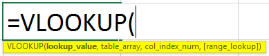
The function accepts four arguments: lookup_value, table_array, col_index_num, and range_lookup. The first three are mandatory arguments, while the last one is optional.
- lookup_value: Required. It represents the value we want to look for in the first column of a table or dataset.
- table_array: Required. It represents the dataset or data array that is to be searched.
- col_index_num: Required. It represents the integer specifying the column number of the table_array that we want to return a value from.
- range_lookup: Optional. It represents or defines what the function should return if it does not find an exact match to the lookup_value. This argument can be set to “FALSE” or “TRUE,” where ‘TRUE’ indicates an approximate match (uses the closest match below the lookup_value in case the exact match is not found), and “FALSE” indicates an exact match (it returns an error in case the exact match is not found). “TRUE” can also be substituted for “1” and “FALSE” for “0.”
How to Use VLOOKUP in Excel?
Let us go through a few examples of VLOOKUP in Excel. They will be beneficial for both beginners and advanced Excel users.
You can download this VLOOKUP Excel Template here – VLOOKUP Excel Template
Example #1
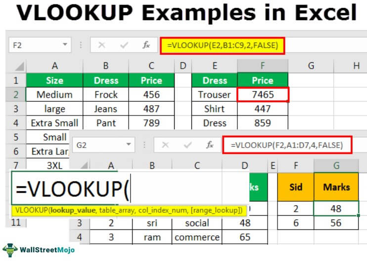
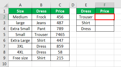
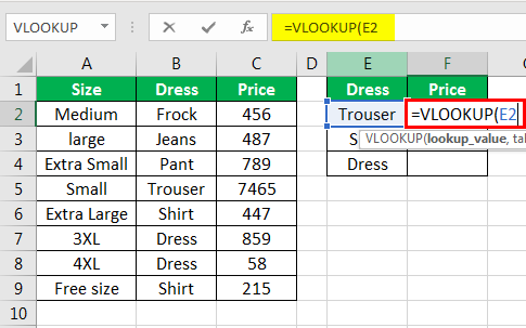
The following table shows the prices of various types of dresses. We want to find the price of the trouser, shirt, and dress.

Time needed: 2 minutes.
The steps to use the VLOOKUP Excel function are listed as follows:
- First, organize the data in the left to right format because the function works in this order. Such an arrangement (shown in the next image) makes it easy to use the VLOOKUP function.
- Place the cursor where the formula is to be entered. For example, since the trouser price is to be found, we place the cursor in cell F2, as shown in the next image.

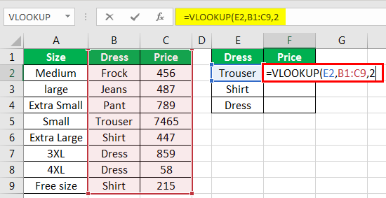
- Enter the formula “=VLOOKUP(E2,B1:C9,2,FALSE)”. It is essential to supply correct arguments to the function to find the exact value.

In the following pointers (steps 3a to 3d), all the arguments of the VLOOKUP function concerning the current example are explained one by one.
Step 3(a): Lookup_value – This is the function’s first and main argument. It specifies the value to be searched in the table. So, the “lookup_value” is E2 (trouser).

Step 3(b): Table_array-This refers to the table range in which the lookup value is to be searched. So, the lookup value is to be searched in the range B1:C9 of the lookup table.

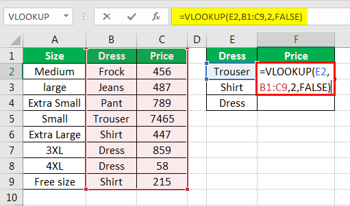
Step 3(c): Col_index_num-This is the index number of the column. It specifies the column from which the value is to be returned. For example, the word “trouser” is present in column B (column 2).
So, this argument is 2, referring to the second column of the table array.
Note: The leftmost column of the table array is counted as 1.

Step 3(d): Range_lookup-This is the Boolean value “True” or “False.” The values are explained as follows:
• True – It is used for an approximate or a close match. The data is matched with the argument approximately. For instance, the first word is looked up if the data contains more than one word.
• False – It is used for an exact match. All the words in the data are matched, and a corresponding value is returned.Hence, we enter “False” because we want the formula to return an exact match. The complete formula is shown in the next image.
Note: If the “range_lookup” argument is omitted, the default value is “True.”
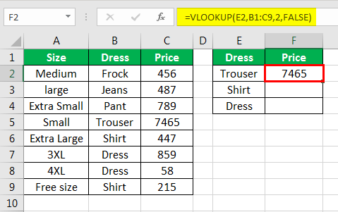
- Press the “Enter” key. All the arguments have been passed correctly. The result is displayed in the following image.

- Drag the formula to obtain the prices of the shirt and dress. The output is shown in the following image.


Example #2
The following table shows the marks of 6 students in different subjects. The serial ID (Sid) number is in the first column (A).
We want to find the marks corresponding to serial ID numbers 2 and 6.

The steps to apply the VLOOKUP function are listed as follows:
Step 1: Organize the data and place the cursor in cell G2, where we will enter the formula.
Step 2: Enter the VLOOKUP Excel formula in cell G2. For auto-populating, the formula, press the “tab” key.

Step 3: Enter the function’s first argument, as shown in the next image. The “lookup_value” is cell F2. It is the value we are looking for.
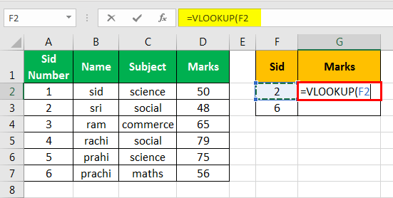
Step 4: Enter the next argument, the table_array. Select A1:D7 as shown in the following image. It is the source table where the serial ID is to be found.

Step 5: Enter the col_index_num, the serial number of the column from which the value is to be returned. Since we want the function to return a value from the “marks” column, we type 4.
The serial ID number column (A) is counted as 1.

Step 6: Enter the argument “range_lookup,” which consists of two values, “True” or “False.” Since the latter value returns an exact match, we type “False.” Finally, close the brackets of the formula.
The exact match option (False) is usually used to avoid confusion. The complete formula is shown in the following image.

Step 7: Press the “Enter” key as the formula is ready to be applied. The output is shown in the following image. Drag the formula of cell G2 to obtain the result in cell G3.

Example #3
The next table shows the names of 6 people along with their gender. The serial numbers are given in column A (Sno).
We want to find the serial number of a given gender.
The formula “=VLOOKUP(E2,A1:C7,1,FALSE)” returns the output #N/A error.
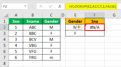
We want to find the serial number for the given gender. The lookup_value is E2 meaning the value to be looked up (gender) is to the right side of the serial number column (A).
The VLOOKUP function does not work because it looks for values beginning from left to right. Simply put, the lookup column (gender) should always be to the left of the return column (serial number or Sno).
The function searches the leftmost column of the “table_array” and returns a corresponding value from the right-hand side column.
The #N/A error is the “value not available” error, as shown in the next image.
Note 1: The limitation of the VLOOKUP function in Excel is that it works on columns from left to right.
Note 2: Using the VLOOKUP to extract values from the leftVlookup to the left finds the respective values which are in the left column of the reference cell. Index, and match are such formulas which are combined together or we can use conditional formulas in the lookup function to find values to the left.read more, is combined with the IF and CHOOSE functionsChoose Function returns a value from the list of values in a given range. This function takes two mandatory arguments: the index number and the first value. The other values are optional to mention.read more.

The Characteristics of VLOOKUP Function
- It is not case-sensitive, implying that the uppercase and lowercase alphabets are treated the same.
- When duplicate values are absent, we should use them for a given data table. If duplicate matches are found, the function returns only the first one.
- It is often used in financial calculations.
The VLOOKUP Errors in Excel
The VLOOKUP formula returns errors on account for various reasons. There are three types of VLOOKUP errorsThe top four VLOOKUP errors are — #N/A Error, #NAME? Error, #REF! Error, #VALUE! Error.read more which are explained as follows:
“#N/A!” error – This occurs if the function cannot find the “lookup_value” in the given “table_array.”
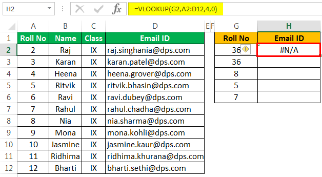
“#REF!” error – This error occurs if the supplied col_index_ num argument exceeds the number of columns in the table_array.”
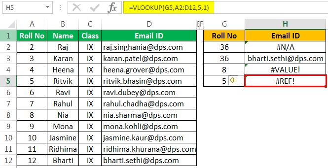
“#VALUE!” error – It occurs if the col_index_ num argument is not given or is supplied as less than 1.
Frequently Asked Questions
How to use VLOOKUP function for a partial match?
We can use the function to search for text beginning or ending with particular alphabets. For instance, we want to find a person’s name that begins with “eli.” The formula is stated as follows:
“=VLOOKUP(“eli*”,table_array,col_index_num,range_lookup)
Hence, the formula will search the “table_array” for names beginning with “eli.”
How to use VLOOKUP formula for absolute and relative cell references?
In most cases, the table_array is locked with the dollar sign ($) like $A$2:$B$10 because it prevents the array from changing while copying the formula to different cells.
Usually, the lookup_value” is supplied as a relative reference like C2. It adjusts the reference as the formula is copied to different cells. It is also possible to lock the column coordinate like $C2.
Give examples of the VLOOKUP excel function.
All example headings are followed by their respective formulas in the given pointers.
Example 1 – To extract data from a different worksheet “=VLOOKUP(lookup_value, sheetname!table_array,col_index_num,range_lookup)”
• Example 2 – To extract data from a different workbook
“=VLOOKUP(lookup_value, workbookname.xlsx]sheetname!table_array,col_index_num,range_lookup)”
Note: If the workbook or the worksheet name contains spaces or non-alphabetical letters, enclose it within single quotes.
• Example 3 – To extract data from a named range “=VLOOKUP(lookup_value,name_range,col_index_num,range_lookup)”
Note: If the name range pertains to a different workbook, enter the latter’s name before the former’s.
Recommended Articles
This article is a guide for VLOOKUP Excel Function. Here, we discuss using the VLOOKUP formula along with step-by-step examples. You may learn more about Excel from the following articles: –
- VLOOKUP in Pivot TableTo use VLOOKUP in a pivot table, select the reference cell as the lookup value, and for the table array arguments, select the data in the pivot table, then identify the column number that has the output, and then give the command based on the close match.read more
- Excel LOOKUP FormulaThe LOOKUP excel function searches a value in a range (single row or single column) and returns a corresponding match from the same position of another range (single row or single column). The corresponding match is a piece of information associated with the value being searched.
read more - VLOOKUP with SUMVlookup is a very versatile function combined with other functions to get some desired result. One such situation is calculating the sum of the data (in numbers) based on matching values. We can combine the sum function with the Vlookup function as =SUM(Vlookup(reference value, table array, index number, match))read more
- IF Statement with VLOOKUPIn Excel, vlookup is a reference function, and IF is a conditional statement. Based on the results of the Vlookup function, they locate a value that meets the criteria and also matches the reference value.read more
Author: Oscar Cronquist Article last updated on February 22, 2023
I will in this article demonstrate how to use the VLOOKUP function with multiple conditions. The function was not built for these circumstances, however, I will demonstrate a few workarounds and also explain how they work.
There is a file for you to get at the very end of this article.
Table of Contents
VLOOKUP examples
- VLOOKUP function with two conditions applied to two columns (AND logic)?
- VLOOKUP function with two conditions applied to two columns (OR logic)?
- VLOOKUP function with many conditions applied to one column (OR logic)?
- Can we use VLOOKUP with multiple lookup values?
- VLOOKUP across multiple columns?
- Can you concatenate VLOOKUP results?
- How to use VLOOKUP with dates?
- What if I don’t have the lookup column in the left-most column?
- VLOOKUP — Select column using a drop-down list
- Why do I want to convert the data set to an Excel Table?
XLOOKUP examples
- XLOOKUP — two conditions in two columns (AND logic)?
- XLOOKUP — two conditions in two columns (OR logic)?
- XLOOKUP — multiple conditions in one column (OR logic)?
- Can we use XLOOKUP with multiple lookup values?
- XLOOKUP across multiple columns?
- Can you concatenate XLOOKUP results?
- How to use XLOOKUP with dates?
- What if I don’t have the lookup column in the left-most column?
1.1 How to use the VLOOKUP function with two conditions (AND logic)?
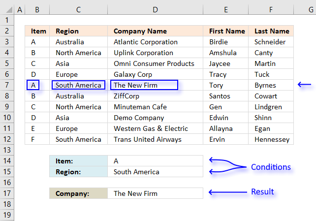
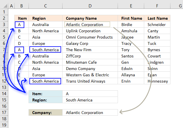
The image above shows a data set in cell range B2:F12, the VLOOKUP function in cell D16 looks for both a value in column B and another value in column C. If both values match a third value on the same row is retrieved from column D and shown in cell D17.
AND logic means that the VLOOKUP function retrieves only if both conditions match.
Can you combine the IF function and the VLOOKUP function?
Yes, you can, in fact, it is the easiest way to VLOOKUP using two or more conditions.
Array formula in D17:
=VLOOKUP(D14, IF(C3:C12=D15, B3:F12, «»), 3, FALSE)
To enter an array formula press and hold CTRL + SHIFT simultaneously, then press Enter once. Release all keys.
The formula bar now shows the formula enclosed with curly brackets telling you that you entered the formula successfully. Don’t enter the curly brackets yourself.
Explaining formula in cell D17
I recommend you use the «Evaluate Formula» feature in Excel to examine calculations step by step.
Select cell D17, go to tab «Formulas» on the ribbon and press with left mouse button on the «Evaluate Formula» button.
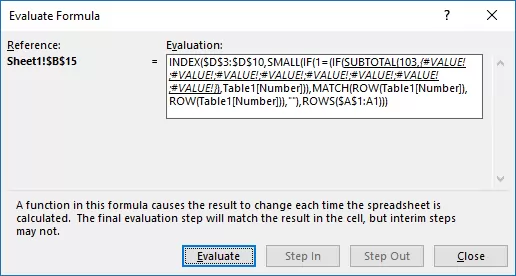
(The formula shown in the above image is not the formula used in this article.)
Press with left mouse button on «Evaluate» button to see the next step in the formula calculations.
Step 1 — Filter records
The IF function filters records that match the value in cell D15, all remaining records are blank. The IF function has three arguments: IF(logical_test, [value_if_true], [value_if_false])
The logical_test argument is C3:C12=D15, it checks if the values in column C are equal to the condition in cell D15. TRUE is returned if it is equal and FALSE if not equal.
IF(C3:C12=D15, B3:F12, «»)
becomes
IF({«Australia»; «North America»; «Asia»; «Europe»; «South America»; «Australia»; «North America»; «Asia»; «Europe»; «South America»}=»South America», B3:F12, «»)
becomes
IF({FALSE; FALSE; FALSE; FALSE; TRUE; FALSE; FALSE; FALSE; FALSE; TRUE}, B3:F12, «»)
If a value in the array is TRUE the corresponding values in B3:F12 are returned and FALSE returns a blank row.
IF({FALSE; FALSE; FALSE; FALSE; TRUE; FALSE; FALSE; FALSE; FALSE; TRUE}, B3:F12, «»)
becomes
IF({FALSE; FALSE; FALSE; FALSE; TRUE; FALSE; FALSE; FALSE; FALSE; TRUE},{«A»,»Australia»,»Atlantic Corporation»,»Birdie»,»Schneider»; «B»,»North America»,»Uplink Corporation»,»Amshula»,»Canty»; «C»,»Asia»,»Omni Consumer Products»,»Jaycee»,»Martin»; «D»,»Europe»,»Galaxy Corp»,»Tracy»,»Tuck»; «A»,»South America»,»The New Firm»,»Tory»,»Byrnes»; «B»,»Australia»,»ZiffCorp»,»Santos»,»Cowart»; «C»,»North America»,»Minuteman Cafe»,»Gen»,»Lindgren»; «D»,»Asia»,»Demo Company»,»Edwin»,»Shinn»; «E»,»Europe»,»Western Gas & Electric»,»Allayna»,»Egan»; «F»,»South America»,»Trans United Airways»,»Ervin»,»Hennessey»}, «»)
and returns
{«»,»»,»»,»»,»»;»»,»»,»»,»»,»»;»»,»»,»»,»»,»»;»»,»»,»»,»»,»»;»A»,»South America»,»The New Firm»,»Tory»,»Byrnes»;»»,»»,»»,»»,»»;»»,»»,»»,»»,»»;»»,»»,»»,»»,»»;»»,»»,»»,»»,»»;»F»,»South America»,»Trans United Airways»,»Ervin»,»Hennessey»}
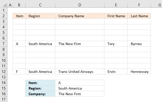
This array has commas and semicolons as delimiting characters, the picture below shows the array in cell range B3:F12. It is now obvious that the IF function has filtered records containing ony the condition.
Step 2 — VLOOKUP value and return value from column to cell D16
VLOOKUP(D14,IF(C3:C12=D15,B3:F12,»»),3,FALSE)
becomes
VLOOKUP(D14, {«», «», «», «», «»; «», «», «», «», «»; «», «», «», «», «»; «», «», «», «», «»; «A», «South America», «The New Firm», «Tory», «Byrnes»; «», «», «», «», «»; «», «», «», «», «»; «», «», «», «», «»; «», «», «», «», «»; «F», «South America», «Trans United Airways», «Ervin», «Hennessey»}, 3, FALSE)
and returns «The New Firm» in cell D16.
Back to top
1.2 How to use the VLOOKUP function with two conditions applied to two columns (OR logic)?
This example demonstrates a formula that returns a value from a record that matches at least one of the two conditions, that is why it is called OR logic.
It becomes quite quickly obvious that the VLOOKUP function is not built for more advanced criteria, I am not using the VLOOKUP function in this example, to keep the formula as small as possible.
Array formula in cell D17:
=INDEX($D$3:$D$12,MATCH(TRUE,(B3:B12=D14)+(C3:C12=D15)>0,0))
To enter an array formula press and hold CTRL + SHIFT simultaneously, then press Enter once. Release all keys.
The formula bar now shows the formula enclosed with curly brackets telling you that you entered the formula successfully. Don’t enter the curly brackets yourself.
If you are looking for a non-array formula here is one:
=LOOKUP(2,1/((B3:B12=D14)+(C3:C12=D15)),D3:D12)
This formula returns a value from the last matching record contrary to the first formula above that returns a value from the first matching record.
Explaining formula in cell D17
Step 1 — First condition
The first condition is specified in cell D14, to compare that value with the values in cell range B3:B14 I use the equal sign. It is a logical operator that returns TRUE or FALSE after the evaluations is made.
We are performing multiple calcualtions in one cell and this is the reason we need to enter this as an array formula.
B3:B12=D14
becomes
{«A»;»B»;»C»;»D»;»A»;»B»;»C»;»D»;»E»;»F»}=»A»
and returns
{TRUE; FALSE; FALSE; FALSE; TRUE; FALSE; FALSE; FALSE; FALSE; FALSE}
Step 2 — Second condition
C3:C12=D15
becomes
{«Australia»;»North America»;»Asia»;»Europe»;»South America»;»Australia»;»North America»;»Asia»;»Europe»;»South America»}=»South America»
and returns
{FALSE; FALSE; FALSE; FALSE; TRUE; FALSE; FALSE; FALSE; FALSE; TRUE}
Step 3 — Add arrays to apply OR logic
The plus sign adds the two arrays row-wise, TRUE + TRUE = 2, TRUE + FALSE = 1 and FALSE + FALSE = 0
((B3:B12=D14)+(C3:C12=D15))>0
becomes
({TRUE; FALSE; FALSE; FALSE; TRUE; FALSE; FALSE; FALSE; FALSE; FALSE} + {FALSE; FALSE; FALSE; FALSE; TRUE; FALSE; FALSE; FALSE; FALSE; TRUE})>0
becomes
{1;0;0;0;2;0;0;0;0;1}>0
and returns
{TRUE; FALSE; FALSE; FALSE; TRUE; FALSE; FALSE; FALSE; FALSE; TRUE}
Step 4 — Identify the position
The MATCH function, as it is set up in this example, returns the relative position of the first found matching value based on an exact match.
MATCH(TRUE,((B3:B12=D14)+(C3:C12=D15))>0,0)
becomes
MATCH(TRUE,{TRUE; FALSE; FALSE; FALSE; TRUE; FALSE; FALSE; FALSE; FALSE; TRUE},0)
and returns 1.
Step 5 — Return the corresponding value
The INDEX function returns a value based on a row and column number.
INDEX($D$3:$D$12, MATCH(TRUE, ((B3:B12=D14)+(C3:C12=D15))>0, 0))
becomes
INDEX($D$3:$D$12, 1)
and returns «Atlantic Corporation» in cell D17.
Back to top
1.3 How to use the VLOOKUP function with many conditions applied to one column (OR logic)?
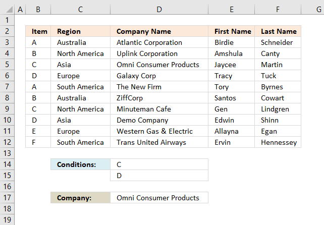
This example demonstrates how to use multiple conditions and the formula returns a value from the first record that matches any of the conditions.
The following formula does not use the VLOOKUP function, it is possible to build such formula but it will be complicated and much larger than needed.
Array formula in cell D17:
=INDEX($D$3:$D$12, MATCH(1, COUNTIF(D14:D15, B3:B12), 0))
To enter an array formula press and hold CTRL + SHIFT simultaneously, then press Enter once. Release all keys.
The formula bar now shows the formula enclosed with curly brackets telling you that you entered the formula successfully. Don’t enter the curly brackets yourself.
Explaining formula in cell D17
Step 1 — Check values that match
The COUNTIF function counts values that equal a condition, however, it can also count multiple conditions but we must enter this formula as an array formula in order to calculate multiple values in one cell.
COUNTIF(D14:D15, B3:B12)>0
becomes
COUNTIF({«C»;»D»},{«A»;»B»;»C»;»D»;»A»;»B»;»C»;»D»;»E»;»F»})
and returns
{0;0;1;1;0;0;1;1;0;0}.
This array has as many values as there are values in cell range B3:B12, the values also corresponds to B3:B12. 0 (zero) indicates that the value is not equal to «C» or «D» and 1 shows that the value is equal to «C» or «D».
Step 2 — Find the position of the record
The MATCH function, as it is set up in this example, returns the relative position of the first found matching value based on an exact match.
MATCH(1, COUNTIF(D14:D15, B3:B12), 0)
becomes
MATCH(1, {0;0;1;1;0;0;1;1;0;0}, 0)
and returns 3. The first value that is equal to 1 is in 3rd position in the array.
Step 3 — Return corresponding value
The INDEX function returns a value based on a row and column number, the cell range is in a column only, we don’t need to specify the column number.
INDEX($D$3:$D$12, MATCH(1, COUNTIF(D14:D15, B3:B12), 0))
becomes
INDEX($D$3:$D$12, 3)
and returns «Omni Consumer Products».
Back to top
1.4 How to use VLOOKUP function with multiple lookup values?
This example demonstrates how to use multiple lookup values in the VLOOKUP function, the lookup values are in cell D14 and D15.
The lookup values are found in row 5,6,9 and 10 but only the corresponding values from row 5 and 6 are returned, that is how the VLOOKUP function is supposed to work. If you need to extract multiple values based on a condition read this: 5 easy ways to VLOOKUP and return multiple values
Array formula in cell D14:D15:
=VLOOKUP(D14:D15, B3:F12, 3, FALSE)
This is an array formula, it returns multiple values. We need to enter it in multiple cells at once, here is how to do it.
Select cell range D14:D15, press with left mouse button on in the formula bar to see the prompt. Copy and paste above array formula to formula bar.
To enter an array formula press and hold CTRL + SHIFT simultaneously, then press Enter once. Release all keys.
The formula bar now shows the formula enclosed with curly brackets telling you that you entered the formula successfully. Don’t enter the curly brackets yourself.
The VLOOKUP function demonstrated above has two lookup values which is fine as long as you enter it in as many cells as there are lookup values.
The downside with this formula is that it only extracts one return value per lookup value, read this article: Vlookup with 2 or more lookup criteria and return multiple matches
Back to top
1.5 VLOOKUP across multiple columns?
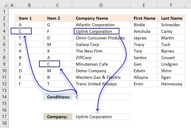
Unfortunately, the VLOOKUP function can’t look in other columns than the left-most column in a cell range. We need to use other functions to accomplish that.
The image above demonstrates an array formula in cell D17 that returns a value from column D (Company Name) if the corresponding value on the same row in column B or C matches the specified value in cell D17.
Array formula in cell D17:
=INDEX($D$3:$D$12,MIN(IF(B3:C12=D14,MATCH(ROW(B3:B12),ROW(B3:B12)),»»)))
To enter an array formula press and hold CTRL + SHIFT simultaneously, then press Enter once. Release all keys.
The formula bar now shows the formula enclosed with curly brackets telling you that you entered the formula successfully. Don’t enter the curly brackets yourself.
Explaining formula in cell D17
Step 1 — Compare values to the lookup value
The equal sign lets you check if a cell value is equal to another value, the difference with this setup is that it compares a cell value to a cell range.
In this case B3:C12, this is fine as long as you enter the formula as an array formula. The formula performs multiple calcualtions in one cell, the result is an array containing boolean values, TRUE or FALSE.
B3:C12=D14
becomes
{«A»,»G»; «C»,»F»; «T»,»D»; «V»,»M»; «A»,»X»; «B»,»A»; «E»,»C»; «D»,»M»; «E»,»B»; «F»,»T»}=»C»
Values are separated by a comma or semicolon, a comma is a column delimiting character and a semicolon is a row delimiting character.
{«A»,»G»; «C»,»F»; «T»,»D»; «V»,»M»; «A»,»X»; «B»,»A»; «E»,»C»; «D»,»M»; «E»,»B»; «F»,»T»}=»C»
returns
{FALSE,FALSE; TRUE,FALSE; FALSE,FALSE; FALSE,FALSE; FALSE,FALSE; FALSE,FALSE; FALSE,TRUE; FALSE,FALSE; FALSE,FALSE; FALSE,FALSE}
Step 2 — Replace boolean values with corresponding row number
The IF function allows you to change the array based on if the logical expression returns TRUE or FALSE.
IF(B3:C12=D14,MATCH(ROW(B3:B12),ROW(B3:B12)),»»)
becomes
IF({FALSE,FALSE; TRUE,FALSE; FALSE,FALSE; FALSE,FALSE; FALSE,FALSE; FALSE,FALSE; FALSE,TRUE; FALSE,FALSE; FALSE,FALSE; FALSE,FALSE}, MATCH(ROW(B3:B12), ROW(B3:B12)),»»)
becomes
IF({FALSE,FALSE; TRUE,FALSE; FALSE,FALSE; FALSE,FALSE; FALSE,FALSE; FALSE,FALSE; FALSE,TRUE; FALSE,FALSE; FALSE,FALSE; FALSE,FALSE}, {1;2;3;4;5;6;7;8;9;10}), «»)
and returns
{«»,»»; 2,»»; «»,»»; «»,»»; «»,»»; «»,»»; «»,7; «»,»»; «»,»»; «»,»»}
Step 3 — Extract the smallest row number
The MIN function returns the samllest number from an cell range or array.
MIN(IF(B3:C12=D14,MATCH(ROW(B3:B12),ROW(B3:B12)),»»)
becomes
MIN({«»,»»; 2,»»; «»,»»; «»,»»; «»,»»; «»,»»; «»,7; «»,»»; «»,»»; «»,»»})
and returns 2.
Step 4 — Return value
The INDEX function returns a value from a cell range or array based on a row and column number. Our example has only a single column so the column number is not needed.
INDEX($D$3:$D$12,MIN(IF(B3:C12=D14,MATCH(ROW(B3:B12),ROW(B3:B12)),»»)))
becomes
INDEX($D$3:$D$12, 2)
and returns «Uplink Corporation».
Back to top
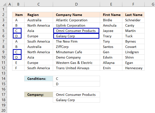
1.6 Can you concatenate VLOOKUP results?
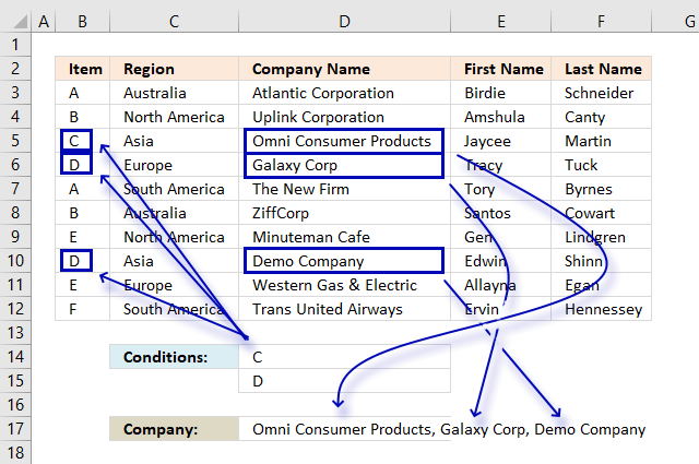
No, you can’t concatenate multiple return values from a VLOOKUP function. It will only return one instance. This example shows how to concatenate multiple values using multiple conditions using the TEXTJOIN, IF and COUNTIF functions.
Array formula in cell D17:
=TEXTJOIN(«, «,TRUE, IF(COUNTIF(D14:D15,B3:B12),D3:D12,»»))
To enter an array formula press and hold CTRL + SHIFT simultaneously, then press Enter once. Release all keys.
The formula bar now shows the formula enclosed with curly brackets telling you that you entered the formula successfully. Don’t enter the curly brackets yourself.
Explaining formula in cell D17
Step 1 — Determine which records match the conditions
The COUNTIF function counts values equal a condition or in this case multiple conditions.
COUNTIF(D14:D15,B3:B12)
becomes
COUNTIF({«C»; «D»} ,{«A»; «B»; «C»; «D»; «A»; «B»; «E»; «D»; «E»; «F»})
and returns {0; 0; 1; 1; 0; 0; 0; 1; 0; 0}.
Step 2 — Replace array with values
The IF function allows you to change the array based on if the logical expression returns TRUE or FALSE.
IF(COUNTIF(D14:D15,B3:B12),D3:D12,»»)
becomes
IF({0; 0; 1; 1; 0; 0; 0; 1; 0; 0}, D3:D12, «»)
becomes
IF({0; 0; 1; 1; 0; 0; 0; 1; 0; 0}, {«Atlantic Corporation»; «Uplink Corporation»; «Omni Consumer Products»; «Galaxy Corp»; «The New Firm»; «ZiffCorp»; «Minuteman Cafe»; «Demo Company»; «Western Gas & Electric»; «Trans United Airways»}, «»)
and returns
{«»;»»;»Omni Consumer Products»;»Galaxy Corp»;»»;»»;»»;»Demo Company»;»»;»»}
Step 3 — Concatenate values
The TEXTJOIN function allows you to concatenate a cell range or array, you can choose the delimiting character and if you want to ignore blank values.
TEXTJOIN(«, «,TRUE, IF(COUNTIF(D14:D15,B3:B12),D3:D12,»»))
becomes
TEXTJOIN(«, «,TRUE, {«»;»»;»Omni Consumer Products»;»Galaxy Corp»;»»;»»;»»;»Demo Company»;»»;»»})
and returns «Omni Consumer Products, Galaxy Corp».
Back to top
1.7 How to use VLOOKUP with dates?
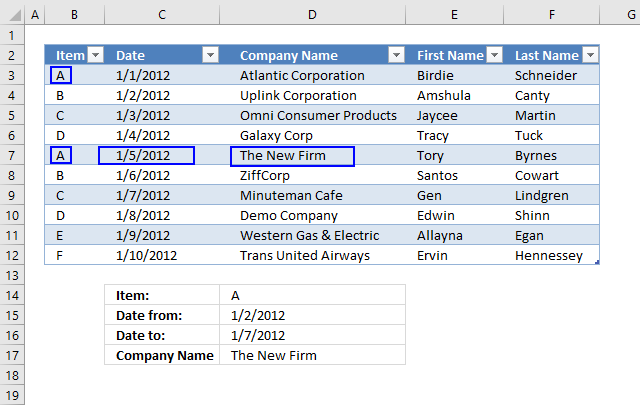
This example shows how to VLOOKUP using a condition, start and end date. The formula returns a value from the first record that matches all three conditions.
Array formula in cell C5:
=VLOOKUP(C2,IF((Table3[Date]>=C3)*(Table3[Date]<=C4),Table3,»»),3,FALSE)
To enter an array formula press and hold CTRL + SHIFT simultaneously, then press Enter once. Release all keys.
The formula bar now shows the formula enclosed with curly brackets telling you that you entered the formula successfully. Don’t enter the curly brackets yourself.
Explaining formula in cell C5
Step 1 — Identify rows with dates larger than the start date
This logical expression checks whether the dates in column Date are bigger (later) than the start date in cell C3.
Table3[Date]>=C3
becomes
{40909; 40910; 40911; 40912; 40913; 40914; 40915; 40916; 40917; 40918}>=40910
and returns
{FALSE; TRUE; TRUE; TRUE; TRUE; TRUE; TRUE; TRUE; TRUE; TRUE}
Step 2 — Identify rows with dates smaller than the end date
The following logical expression checks whether the dates in column Date are smaller (earlier) than the end date in cell C3.
Table3[Date]<=C4
becomes
{40909;40910;40911;40912;40913;40914;40915;40916;40917;40918}<=40915
and returns
{TRUE;TRUE;TRUE;TRUE;TRUE;TRUE;TRUE;FALSE;FALSE;FALSE}
Step 3 — Multiply arrays
We want to know if both conditions are met, to do that we must multiply the arrays. TRUE * TRUE = TRUE (1), TRUE * FALSE = FALSE (0), FALSE * FALSE = FALSE (0)
(Table3[Date]>=C3)*(Table3[Date]<=C4)
becomes
{FALSE; TRUE; TRUE; TRUE; TRUE; TRUE; TRUE; TRUE; TRUE; TRUE} * {TRUE; TRUE; TRUE; TRUE; TRUE; TRUE; TRUE; FALSE; FALSE; FALSE}
returns
{0;1;1;1;1;1;1;0;0;0}
Step 4 — Filter records that match
The IF function filters records that match both conditions.
IF((Table3[Date]>=C3)*(Table3[Date]<=C4),Table3,»»)
becomes
IF({0; 1; 1; 1; 1; 1; 1; 0; 0; 0},Table3,»»)
and returns
{«»,»»,»»,»»,»»; «B»,40910,»Uplink Corporation»,»Amshula»,»Canty»; «C»,40911,»Omni Consumer Products»,»Jaycee»,»Martin»; «D»,40912,»Galaxy Corp»,»Tracy»,»Tuck»; «A»,40913,»The New Firm»,»Tory»,»Byrnes»; «B»,40914,»ZiffCorp»,»Santos»,»Cowart»; «C»,40915,»Minuteman Cafe»,»Gen»,»Lindgren»; «»,»»,»»,»»,»»; «»,»»,»»,»»,»»; «»,»»,»»,»»,»»}.
Step 5 — VLOOKUP using the array
The VLOOKUP function uses the array returned from the IF function and looks for the lookup value in the left-most column in the array.
VLOOKUP(C2,IF((Table3[Date]>=C3)*(Table3[Date]<=C4),Table3,»»),3,FALSE)
becomes
VLOOKUP(C2,IF({0;1;1;1;1;1;1;0;0;0},Table3,»»),3,FALSE)
becomes
VLOOKUP(C2,IF({0;1;1;1;1;1;1;0;0;0},{«A», 40909, «Atlantic Corporation», «Birdie», «Schneider»;»B», 40910, «Uplink Corporation», «Amshula», «Canty»;»C», 40911, «Omni Consumer Products», «Jaycee», «Martin»;»D», 40912, «Galaxy Corp», «Tracy», «Tuck»;»A», 40913, «The New Firm», «Tory», «Byrnes»;»B», 40914, «ZiffCorp», «Santos», «Cowart»;»C», 40915, «Minuteman Cafe», «Gen», «Lindgren»;»D», 40916, «Demo Company», «Edwin», «Shinn»;»E», 40917, «Western Gas & Electric», «Allayna», «Egan»;»F», 40918, «Trans United Airways», «Ervin», «Hennessey»},»»),3,FALSE)
becomes
VLOOKUP(«A»,{«»,»»,»»,»»,»»;»B»,40910,»Uplink Corporation»,»Amshula»,»Canty»;»C»,40911,»Omni Consumer Products»,»Jaycee»,»Martin»;»D»,40912,»Galaxy Corp»,»Tracy»,»Tuck»;»A»,40913,»The New Firm»,»Tory»,»Byrnes»;»B»,40914,»ZiffCorp»,»Santos»,»Cowart»;»C»,40915,»Minuteman Cafe»,»Gen»,»Lindgren»;»»,»»,»»,»»,»»;»»,»»,»»,»»,»»;»»,»»,»»,»»,»»},3,FALSE)
and returns «The New Firm»
Back to top
1.8 What if I don’t have the lookup column in the left-most column?

The VLOOKUP function can only look for values in the first column of the table_array. The formula below demonstrates how to do a lookup in any table column and return a value from any table column.
The INDEX and MATCH function is more versatile than VLOOKUP and it is easier to apply more conditions if needed, however, it still can only return one value even if there are more records that match. The INDEX, SMALL and IF function can return multiple values, read this article: 5 easy ways to VLOOKUP and return multiple values
Formula in cell C3:
=INDEX(Table4[Item],MATCH(C2,Table4[First Name],0))
Learn more about the INDEX and MATCH functions:
Recommended articles
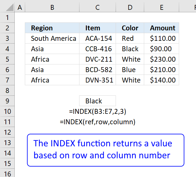
Recommended articles
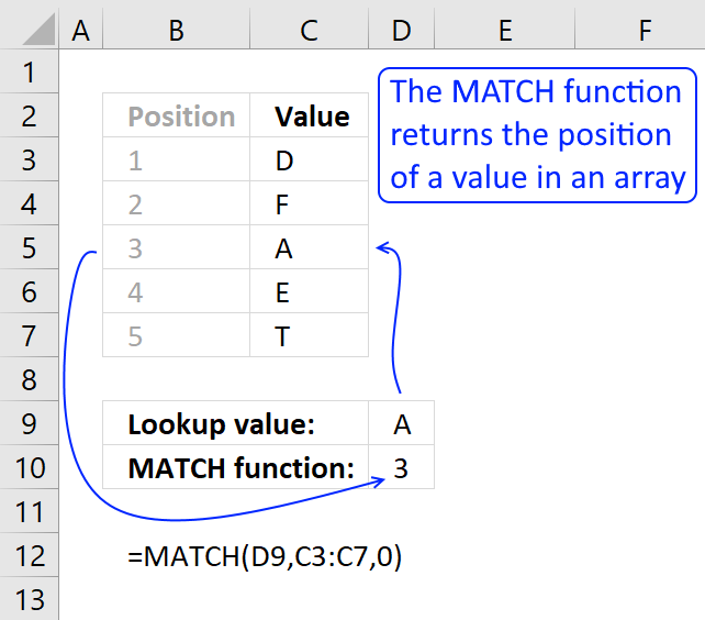
becomes
INDEX(Table4[Item],4)
becomes
INDEX({«A»; «B»; «C»; «D»; «A»; «B»; «C»; «D»; «E»; «F»},4)
and returns D in cell C3.
Back to top
1.9 VLOOKUP — Select column using a drop-down list

The worksheet shown above lets you select the column using a drop-down list from which you want the return value, this way you don’t need to edit the formula when you need data from another column.
Array formula in cell C4:
=VLOOKUP(C2, IF(Table2[Region]=C3, Table2, «»), MATCH(B4, Table2[#Headers], 0), FALSE)
How to create the drop down list in cell B4
- Select cell B4
- Go to «Data» tab
- Press with left mouse button on «Data Validation» button
- Select «List» i the drop down list
- Select source: =$C$8:$E$8

- Press with left mouse button on OK

Explaining formula in cell C4
Step 1 — Find the relative position
The MATCH function returns the relative position of an item in an array that matches a specified value in a specific order.
Function syntax: MATCH(lookup_value, lookup_array, [match_type])
MATCH(B4, Table2[#Headers], 0)
becomes
MATCH(Company Name», {«Item»,»Region»,»Company Name»,»First Name»,»Last Name»}, 0)
and returns 3.
Step 2 — Logical test
The equal sign is a logical operator, it lets you compare a value to another value in an Excel formula. The result is a boolean value, TRUE or FALSE.
You can use the equal sign to compare a value to a cell range of values as well.
Table2[Region]=C3
becomes
{«Australia»; «North America»; «Asia»; «Europe»; «South America»; «Australia»; «North America»; «Asia»; «Europe»; «South America»}=»South America»
and returns
{FALSE; FALSE; FALSE; FALSE; TRUE; FALSE; FALSE; FALSE; FALSE; TRUE}
Step 3 — Filter values based on a condition
The IF function returns one value if the logical test is TRUE and another value if the logical test is FALSE.
Function syntax: IF(logical_test, [value_if_true], [value_if_false])
IF(Table2[Region]=C3, Table2, «»)
becomes
IF({FALSE; FALSE; FALSE; FALSE; TRUE; FALSE; FALSE; FALSE; FALSE; TRUE}, Table2, «»)
and returns
{«»,»»,»»,»»,»»; «»,»»,»»,»»,»»; «»,»»,»»,»»,»»; «»,»»,»»,»»,»»; «A»,»South America»,»The New Firm»,»Tory»,»Byrnes»; «»,»»,»»,»»,»»; «»,»»,»»,»»,»»; «»,»»,»»,»»,»»; «»,»»,»»,»»,»»; «F»,»South America»,»Trans United Airways»,»Ervin»,»Hennessey»}
Step 4 — Perform a lookup
The VLOOKUP function lets you search the leftmost column for a value and return another value on the same row in a column you specify.
Function syntax: VLOOKUP(lookup_value, table_array, col_index_num, [range_lookup])
VLOOKUP(C2, IF(Table2[Region]=C3, Table2, «»), MATCH(B4, Table2[#Headers], 0), FALSE)
becomes
VLOOKUP(C2, IF(Table2[Region]=C3, Table2, «»), MATCH(Company Name», {«Item»,»Region»,»Company Name»,»First Name»,»Last Name»}, 0), FALSE)
becomes
VLOOKUP(«A», {«»,»»,»»,»»,»»; «»,»»,»»,»»,»»; «»,»»,»»,»»,»»; «»,»»,»»,»»,»»; «A»,»South America»,»The New Firm»,»Tory»,»Byrnes»; «»,»»,»»,»»,»»; «»,»»,»»,»»,»»; «»,»»,»»,»»,»»; «»,»»,»»,»»,»»; «F»,»South America»,»Trans United Airways»,»Ervin»,»Hennessey»}, 3, FALSE)
and returns «The New Firm».
Back to top
1.10 Why do I want to convert the data set to an Excel Table?

If you convert your cell range to a table you can add or remove as many records to the Excel table as you want and the cell reference in the formula is automatically adjusted.
Use the table name and table column name in the VLOOKUP function to achieve this, see the formula bar in the picture above.
How to convert a cell range to an Excel defined Table?
- Select any cell in your data set.
- Go to tab «Insert» on the ribbon.
- Press with left mouse button on «Table» button to open a dialog box.

- Enable «My table has headers».
- Press with left mouse button on OK.
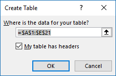
Learn more about excel tables:
Recommended articles
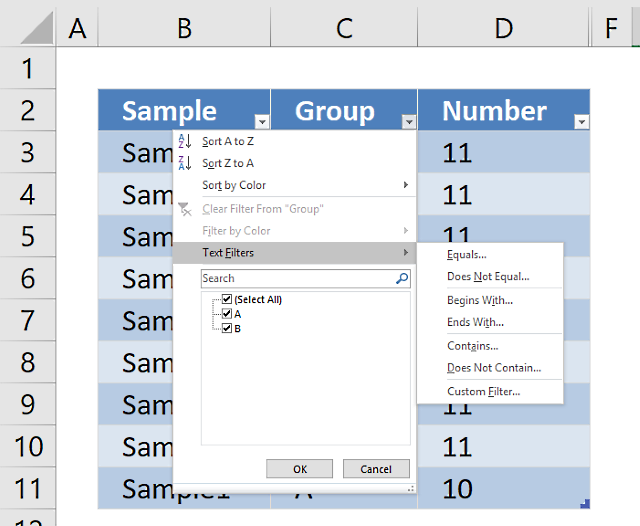
How to use Excel Tables
An Excel table allows you to easily sort, filter and sum values in a data set where values are related.
Back to top
2.1 XLOOKUP function with two conditions applied to two columns (AND logic)?

Excel 365 formula in cell D17:
=XLOOKUP(1,(B3:B12=D14)*(C3:C12=D15),D3:D12)
Explaining formula
Step 1 — First condition
The equal sign is a logical operator, it lets you compare a value to another value in an Excel formula. The result is a boolean value, TRUE or FALSE.
You can use the equal sign to compare a value to a cell range of values as well.
B3:B12=D14
becomes
{«A»;»B»;»C»;»D»;»A»;»B»;»C»;»D»;»E»;»F»}=»A»
and returns
{TRUE; FALSE; FALSE; FALSE; TRUE; FALSE; FALSE; FALSE; FALSE; FALSE}.
Step 2 — Second condition
C3:C12=D15
becomes
{«Australia»; «North America»; «Asia»; «Europe»; «South America»; «Australia»; «North America»; «Asia»; «Europe»; «South America»}=»South America»
and returns
{FALSE; FALSE; FALSE; FALSE; TRUE; FALSE; FALSE; FALSE; FALSE; TRUE}.
Step 3 — Apply AND logic
The parentheses let you control the order of operation. We need to calculate the comparisons before we multiply the arrays.
(B3:B12=D14)*(C3:C12=D15)
becomes
({TRUE; FALSE; FALSE; FALSE; TRUE; FALSE; FALSE; FALSE; FALSE; FALSE})*({FALSE; FALSE; FALSE; FALSE; TRUE; FALSE; FALSE; FALSE; FALSE; TRUE})
and returns
{0;0;0;0;1;0;0;0;0;0}.
Boolean values, when multiplied, return their numerical equivalents. TRUE — 1 and FALSE is 0 (zero).
Here is why AND logic is created when we multiply boolean values, both values must be TRUE in order to return TRUE.
TRUE * TRUE = 1 (TRUE)
TRUE * FALSE = 0 (FALSE)
FALSE * FALSE = 0 (FALSE)
Step 4 — Evaluate XLOOKUP function
The XLOOKUP function search one column for a given value, and return a corresponding value in another column from the same row.
Function syntax: XLOOKUP(lookup_value, lookup_array, return_array, [if_not_found], [match_mode], [search_mode])
XLOOKUP(1,(B3:B12=D14)*(C3:C12=D15),D3:D12)
becomes
XLOOKUP(1, {0;0;0;0;1;0;0;0;0;0},{«Atlantic Corporation»; «Uplink Corporation»; «Omni Consumer Products»; «Galaxy Corp»; «The New Firm»; «ZiffCorp»; «Minuteman Cafe»; «Demo Company»; «Western Gas & Electric»; «Trans United Airways»})
and returns
«The New Firm».
Back to top
2.2 XLOOKUP function with two conditions applied to two columns (OR logic)?

This example shows how to perform lookups in two different columns using two different lookup values respectively. The first record that meets at least one of two conditions is a match, in this example, row 3 is a match and the corresponding value in column D is returned.
Excel 365 formula in cell D17:
=XLOOKUP(TRUE, ((D14=B3:B12)+(D15=C3:C12))>=1, D3:D12)
Explaining formula
Step 1 — First condition
The equal sign is a logical operator, it lets you compare a value to another value in an Excel formula. The result is a boolean value, TRUE or FALSE.
You can use the equal sign to compare a value to a cell range of values as well.
D14=B3:B12
becomes
«A»={«A»; «B»; «C»; «D»; «A»; «B»; «C»; «D»; «E»; «F»}
and returns
{TRUE; FALSE; FALSE; FALSE; TRUE; FALSE; FALSE; FALSE; FALSE; FALSE}
Step 2 — Second condition
D15=C3:C12
becomes
«South America»={«Australia»; «North America»; «Asia»; «Europe»; «South America»; «Australia»; «North America»; «Asia»; «Europe»; «South America»}
and returns
{FALSE; FALSE; FALSE; FALSE; TRUE; FALSE; FALSE; FALSE; FALSE; TRUE}.
Step 3 — Apply OR logic
The parentheses let you control the order of operation. We need to calculate the comparisons before we multiply the arrays.
(D14=B3:B12)+(D15=C3:C12)
becomes
({TRUE; FALSE; FALSE; FALSE; TRUE; FALSE; FALSE; FALSE; FALSE; FALSE}) + ({FALSE; FALSE; FALSE; FALSE; TRUE; FALSE; FALSE; FALSE; FALSE; TRUE})
and returns
{1; 0; 0; 0; 2; 0; 0; 0; 0; 1}.
The plus sign performs addition between two numbers and also boolean values.
TRUE + TRUE = 2 (TRUE)
TRUE + FALSE = 1 (TRUE)
FALSE + FALSE = 0 (FALSE)
Boolean values, when added, are converted to their numerical equivalents.
TRUE — All numbers except zero.
FALSE — 0 (Zero)
Step 4 — Check if numbers are larger than or equal to 1
The larger than sign is a logical operator that lets you compare numbers and also text values if needed. The result is a boolean value, TRUE or FALSE.
((D14=B3:B12)+(D15=C3:C12))>=1
Step 5 — Evaluate XLOOKUP function
The XLOOKUP function search one column for a given value, and return a corresponding value in another column from the same row.
Function syntax: XLOOKUP(lookup_value, lookup_array, return_array, [if_not_found], [match_mode], [search_mode])
XLOOKUP(TRUE, ((D14=B3:B12)+(D15=C3:C12))>=1, D3:D12)
becomes
XLOOKUP(TRUE, {1; 0; 0; 0; 2; 0; 0; 0; 0; 1}, {«Atlantic Corporation»; «Uplink Corporation»; «Omni Consumer Products»; «Galaxy Corp»; «The New Firm»; «ZiffCorp»; «Minuteman Cafe»; «Demo Company»; «Western Gas & Electric»; «Trans United Airways»})
and returns
«Atlantic Corporation».
Back to top
2.3 XLOOKUP — multiple conditions in one column (OR logic)?

This example demonstrates the XLOOKUP function using multiple conditions, however, it returns only a single value from the same row where any of the lookup values are found.
This example shows that the first condition is found before the second condition and the corresponding value on the same row is found in cell D5.
Excel 365 formula in cell D17:
=XLOOKUP(1,COUNTIF(D14:D15,B3:B12),D3:D12)
Explaining formula
Step 1 — Count conditions in each value
The COUNTIF function calculates the number of cells that is equal to a condition.
Function syntax: COUNTIF(range, criteria)
COUNTIF(D14:D15, B3:B12)
becomes
COUNTIF({«C»;»D»}, {«A»;»B»;»C»;»D»;»A»;»B»;»C»;»D»;»E»;»F»})
and returns
{0; 0; 1; 1; 0; 0; 1; 1; 0; 0}.
Step 2 — Lookup based on array
The XLOOKUP function search one column for a given value, and return a corresponding value in another column from the same row.
Function syntax: XLOOKUP(lookup_value, lookup_array, return_array, [if_not_found], [match_mode], [search_mode])
XLOOKUP(1, COUNTIF(D14:D15, B3:B12), D3:D12)
becomes
XLOOKUP(1, {0; 0; 1; 1; 0; 0; 1; 1; 0; 0}, {«Atlantic Corporation»; «Uplink Corporation»; «Omni Consumer Products»; «Galaxy Corp»; «The New Firm»; «ZiffCorp»; «Minuteman Cafe»; «Demo Company»; «Western Gas & Electric»; «Trans United Airways»})
and returns
«Omni Consumer Products».
Back to top
2.4 Can we use XLOOKUP with multiple lookup values?

This example demonstrates the XLOOKUP function also using multiple conditions, however, it returns as many values as there are conditions as long as they match the lookup values..
This example shows the condition in cell D14 is found in cell B5 and the corresponding value in cell D5 is returned to cell D17. The second condition in cell D15 is found in cell B6 and the corresponding value in cell D6 is returned to cell D18.
Excel 365 dynamic formula in cell D17:
=XLOOKUP(D14:D15, B3:B12, D3:D12)
Explaining formula
The XLOOKUP function lets you lookup multiple values in a single formula, the result is an Excel 365 dynamic array that spills values to cells below automatically.
Evaluate XLOOKUP function
The XLOOKUP function search one column for a given value, and return a corresponding value in another column from the same row.
Function syntax: XLOOKUP(lookup_value, lookup_array, return_array, [if_not_found], [match_mode], [search_mode])
XLOOKUP(D14:D15, B3:B12, D3:D12)
becomes
XLOOKUP({«C»; «D»},{«A»; «B»; «C»; «D»; «A»; «B»; «C»; «D»; «E»; «F»},{«Atlantic Corporation»; «Uplink Corporation»; «Omni Consumer Products»; «Galaxy Corp»; «The New Firm»; «ZiffCorp»; «Minuteman Cafe»; «Demo Company»; «Western Gas & Electric»; «Trans United Airways»})
and returns
{«Omni Consumer Products»; «Galaxy Corp»}.
Back to top
2.5 XLOOKUP across multiple columns?

This example performs a lookup across multiple columns using a single lookup value, a value from the first match on the same row is returned, in this example, cells D3:D12.
Excel 365 formula in cell D17:
=XLOOKUP(1, (B3:B12=D14)+(C3:C12=D14), D3:D12)
Explaining formula
Step 1 — First column B
The equal sign is a logical operator, it lets you compare a value to another value in an Excel formula. The result is a boolean value, TRUE or FALSE.
You can use the equal sign to compare a value to a cell range of values as well.
B3:B12=D14
becomes
{«A»; «C»; «T»; «V»; «A»; «B»; «E»; «D»; «E»; «F»}=»C»
and returns
{FALSE; TRUE; FALSE; FALSE; FALSE; FALSE; FALSE; FALSE; FALSE; FALSE}.
Step 2 — Second column C
C3:C12=D14
becomes
{«G»; «F»; «D»; «M»; «X»; «A»; «C»; «M»; «B»; «T»}=»C»
and returns
{FALSE; FALSE; FALSE; FALSE; FALSE; FALSE; TRUE; FALSE; FALSE; FALSE}.
Step 3 — Apply OR logic
The plus sign adds numbers in an Excel formula, it also performs OR logic for boolean values and their numerical equivalents.
TRUE + TRUE = TRUE
TRUE + FALSE = TRUE
FALSE + FALSE = FALSE
OR logic means that at least one boolean value is TRUE in order to return TRUE.
TRUE — Any number except 0 (zero)
FALSE — 0 (zero)
The parentheses lets you control the order of operation, we need to compare the values before we add arrays.
(B3:B12=D14)+(C3:C12=D14)
becomes
({FALSE; TRUE; FALSE; FALSE; FALSE; FALSE; FALSE; FALSE; FALSE; FALSE}) + ({FALSE; FALSE; FALSE; FALSE; FALSE; FALSE; TRUE; FALSE; FALSE; FALSE})
and returns
{0;1;0;0;0;0;1;0;0;0}.
Step 4 — Evaluate XLOOKUP function
The XLOOKUP function search one column for a given value, and return a corresponding value in another column from the same row.
Function syntax: XLOOKUP(lookup_value, lookup_array, return_array, [if_not_found], [match_mode], [search_mode])
XLOOKUP(1,(B3:B12=D14)+(C3:C12=D14),D3:D12)
becomes
XLOOKUP(1,{0; 1; 0; 0; 0; 0; 1; 0; 0; 0}, {«Atlantic Corporation»; «Uplink Corporation»; «Omni Consumer Products»; «Galaxy Corp»; «The New Firm»; «ZiffCorp»; «Minuteman Cafe»; «Demo Company»; «Western Gas & Electric»; «Trans United Airways»})
and returns
«Uplink Corporation».
Back to top
2.6 Can you concatenate XLOOKUP results?

You can concatenate results from the XLOOKUP function, this example demonstrates an XLOOKUP function that lookups two different values, and the results are concatenated using the TEXTJOIN function.
Excel 365 formula in cell D17:
=TEXTJOIN(«, «, TRUE, XLOOKUP(D14:D15, B3:B12, D3:D12))
Explaining formula
Step 1 — Lookup two different values
The XLOOKUP function search one column for a given value, and return a corresponding value in another column from the same row.
Function syntax: XLOOKUP(lookup_value, lookup_array, return_array, [if_not_found], [match_mode], [search_mode])
XLOOKUP(D14:D15,B3:B12,D3:D12)
becomes
XLOOKUP({«C«; «D«}, {«A»; «B»; «C«; «D«; «A»; «B»; «E»; «D»; «E»; «F»}, {«Atlantic Corporation»; «Uplink Corporation»; «Omni Consumer Products«; «Galaxy Corp«; «The New Firm»; «ZiffCorp»; «Minuteman Cafe»; «Demo Company»; «Western Gas & Electric»; «Trans United Airways»})
and returns
{«Omni Consumer Products»; «Galaxy Corp»}.
Step 2 — Join values
The TEXTJOIN function combines text strings from multiple cell ranges.
Function syntax: TEXTJOIN(delimiter, ignore_empty, text1, [text2], …)
TEXTJOIN(«, «,TRUE, XLOOKUP(D14:D15,B3:B12,D3:D12))
becomes
TEXTJOIN(«, «,TRUE, {«Omni Consumer Products»; «Galaxy Corp»})
and returns
«Omni Consumer Products, Galaxy Corp».
Back to top
2.7 How to use XLOOKUP with dates?

This example shows how to use a date range, Excel table, and a condition in the XLOOKUP function. The cell reference (structured reference) to the Excel Table doesn’t change even if you add or delete rows in the table.
Excel 365 formula:
=XLOOKUP(1, (Table35[Date]>=D15)*(Table35[Date]<=D16)*(D14=Table35[Item]), Table35[Company Name])
Explaining formula
Step 1 — Find dates equal or larger than the start date specified in cell D15
The less than and larger than characters are logical operators, they return TRUE or FALSE if the condition is met or not.
Table35[Date]>=D15
becomes
{45658; 45659; 45660; 45661; 45662; 45663; 45664; 45665; 45666; 45667}>=45659
and returns
{FALSE; TRUE; TRUE; TRUE; TRUE; TRUE; TRUE; TRUE; TRUE; TRUE}.
Step 2 — Find dates equal or larger than the end date specified in cell D16
Table35[Date]<=D16
becomes
{45658; 45659; 45660; 45661; 45662; 45663; 45664; 45665; 45666; 45667}>=45664
and returns
{TRUE; TRUE; TRUE; TRUE; TRUE; TRUE; TRUE; FALSE; FALSE; FALSE}.
Step 3 — Find records matching condition specified in cell D14
D14=Table35[Item]
becomes
«A»={«A»; «B»; «C»; «D»; «A»; «B»; «C»; «D»; «E»; «F»}
and returns
{TRUE; FALSE; FALSE; FALSE; TRUE; FALSE; FALSE; FALSE; FALSE; FALSE}.
Step 4 — Apply AND logic
The parentheses let you control the order of operation. We need to calculate the comparisons before we multiply the arrays.
(Table35[Date]>=D15)*(Table35[Date]<=D16)*(D14=Table35[Item])
becomes
({FALSE; TRUE; TRUE; TRUE; TRUE; TRUE; TRUE; TRUE; TRUE; TRUE}) * ({TRUE; TRUE; TRUE; TRUE; TRUE; TRUE; TRUE; FALSE; FALSE; FALSE}) * ({TRUE; FALSE; FALSE; FALSE; TRUE; FALSE; FALSE; FALSE; FALSE; FALSE})
The asterisk character lets you multiply boolean values. When multiplied boolean values return their numerical equivalents. TRUE — 1 and FALSE is 0 (zero).
TRUE * TRUE = 1 (TRUE)
TRUE * FALSE = 0 (FALSE)
FALSE * FALSE = 0 (FALSE)
Both values must be TRUE in order to return TRUE.
({FALSE; TRUE; TRUE; TRUE; TRUE; TRUE; TRUE; TRUE; TRUE; TRUE}) * ({TRUE; TRUE; TRUE; TRUE; TRUE; TRUE; TRUE; FALSE; FALSE; FALSE}) * ({TRUE; FALSE; FALSE; FALSE; TRUE; FALSE; FALSE; FALSE; FALSE; FALSE})
returns
{0; 0; 0; 0; 1; 0; 0; 0; 0; 0}
Step 5 — Evaluate XLOOKUP function
The XLOOKUP function search one column for a given value, and return a corresponding value in another column from the same row.
Function syntax: XLOOKUP(lookup_value, lookup_array, return_array, [if_not_found], [match_mode], [search_mode])
XLOOKUP(1, (Table35[Date]>=D15)*(Table35[Date]<=D16)*(D14=Table35[Item]), Table35[Company Name])
becomes
XLOOKUP(1, {0; 0; 0; 0; 1; 0; 0; 0; 0; 0}, Table35[Company Name])
and returns
«The New Firm».
Back to top
2.8 What if I don’t have the lookup column in the left-most column?

The XLOOKUP function lets you use any lookup column contrary to the VLOOKUP function that requires the leftmost column as the lookup column.
This example demonstrates a lookup column in column C, the leftmost column is column B in the data set.
Formula in cell D15:
=XLOOKUP(D14, C3:C12, D3:D12)
Evaluate XLOOKUP function
The XLOOKUP function search one column for a given value, and return a corresponding value in another column from the same row.
Function syntax: XLOOKUP(lookup_value, lookup_array, return_array, [if_not_found], [match_mode], [search_mode])
XLOOKUP(D14, C3:C12, D3:D12)
becomes
XLOOKUP(«A»,{«A»;»B»;»C»;»D»;»A»;»B»;»C»;»D»;»E»;»F»},{«Atlantic Corporation»;»Uplink Corporation»;»Omni Consumer Products»;»Galaxy Corp»;»The New Firm»;»ZiffCorp»;»Minuteman Cafe»;»Demo Company»;»Western Gas & Electric»;»Trans United Airways»})
and returns
«Atlantic Corporation».
Back to top
Exact Match | Approximate Match | Vlookup Looks Right | First Match | Partial Match | Vlookup is Case-insensitive | Multiple Criteria | #N/A error | Multiple Lookup Tables | Index and Match | Table Magic | Xlookup
The VLOOKUP function is one of the most popular functions in Excel. This page contains many easy to follow VLOOKUP examples.
Exact Match
Most of the time you are looking for an exact match when you use the VLOOKUP function in Excel. Let’s take a look at the arguments of the VLOOKUP function.
1. The VLOOKUP function below looks up the value 53 (first argument) in the leftmost column of the red table (second argument).

2. The value 4 (third argument) tells the VLOOKUP function to return the value in the same row from the fourth column of the red table.

Note: the Boolean FALSE (fourth argument) tells the VLOOKUP function to return an exact match. If the VLOOKUP function cannot find the value 53 in the first column, it will return a #N/A error.
3. Here’s another example. Instead of returning the salary, the VLOOKUP function below returns the last name (third argument is set to 3) of ID 79.

Approximate Match
Let’s take a look at an example of the VLOOKUP function in approximate match mode (fourth argument set to TRUE).
1. The VLOOKUP function below looks up the value 85 (first argument) in the leftmost column of the red table (second argument). There’s just one problem. There’s no value 85 in the first column.

2. Fortunately, the Boolean TRUE (fourth argument) tells the VLOOKUP function to return an approximate match. If the VLOOKUP function cannot find the value 85 in the first column, it will return the largest value smaller than 85. In this example, this will be the value 80.

3. The value 2 (third argument) tells the VLOOKUP function to return the value in the same row from the second column of the red table.

Note: always sort the leftmost column of the red table in ascending order if you use the VLOOKUP function in approximate match mode (fourth argument set to TRUE).
Vlookup Looks Right
The VLOOKUP function always looks up a value in the leftmost column of a table and returns the corresponding value from a column to the right.
1. For example, the VLOOKUP function below looks up the first name and returns the last name.

2. If you change the column index number (third argument) to 3, the VLOOKUP function looks up the first name and returns the salary.

Note: in this example, the VLOOKUP function cannot lookup the first name and return the ID. The VLOOKUP function only looks to the right. No worries, you can use INDEX and MATCH in Excel to perform a left lookup.
First Match
If the leftmost column of the table contains duplicates, the VLOOKUP function matches the first instance. For example, take a look at the VLOOKUP function below.

Explanation: the VLOOKUP function returns the salary of Mia Clark, not Mia Reed.
Partial Match
The VLOOKUP function supports wildcards for partial matches. For example, take a look at the VLOOKUP function below.

Explanation: an asterisk (*) matches zero or more characters. The VLOOKUP function matches the first instance that begins with «Jess». Use «*»&G2 for an «ends with» match. Use «*»&G2&»*» for a «contains» match.
Vlookup is Case-insensitive
The VLOOKUP function in Excel performs a case-insensitive lookup. For example, the VLOOKUP function below looks up MIA (cell G2) in the leftmost column of the table.

Explanation: the VLOOKUP function is case-insensitive so it looks up MIA or Mia or mia or miA, etc. As a result, the VLOOKUP function returns the salary of Mia Clark (first instance). Use INDEX, MATCH and EXACT in Excel to perform a case-sensitive lookup.
Multiple Criteria
Do you want to look up a value based on multiple criteria? Use INDEX and MATCH in Excel to perform a two-column lookup.

Note: the array formula above looks up the salary of James Clark, not James Smith, not James Anderson.
#N/A error
If the VLOOKUP function cannot find a match, it returns a #N/A error.
1. For example, the VLOOKUP function below cannot find the value 28 in the leftmost column.

2. If you like, you can use the IFNA function to replace the #N/A error with a friendly message.

Note: the IFNA function was introduced in Excel 2013. If you’re using Excel 2010 or Excel 2007, combine IF and ISNA or use IFERROR.
Multiple Lookup Tables
When using the VLOOKUP function in Excel, you can have multiple lookup tables. You can use the IF function to check whether a condition is met, and return one lookup table if TRUE and another lookup table if FALSE.
1. Create two named ranges: Table1 and Table2.

2. Select cell E4 and enter the VLOOKUP function shown below.

Explanation: the bonus depends on the market (UK or USA) and the sales amount. The second argument of the VLOOKUP function does the trick. If UK, the VLOOKUP function uses Table1, if USA, the VLOOKUP function uses Table2. Set the fourth argument of the VLOOKUP function to TRUE to return an approximate match.
3. Press Enter.
4. Select cell E4, click on the lower right corner of cell E4 and drag it down to cell E10.

Note: for example, Walker receives a bonus of $1,500. Because we’re using named ranges, we can easily copy this VLOOKUP function to the other cells without worrying about cell references.
Index and Match
Instead of using VLOOKUP, use INDEX and MATCH. To perform advanced lookups, you’ll need INDEX and MATCH. Maybe this is one step too far for you at this stage, but it shows you one of the many other powerful formulas Excel has to offer.

Table Magic
Tables can make VLOOKUP formulas a lot easier. In the example below, a single VLOOKUP function automatically looks up all country codes.

Note: visit our page about merging tables to learn how to create this VLOOKUP function and bring your Excel game to a new level.
Xlookup
If you have Excel 365 or Excel 2021, use XLOOKUP instead of VLOOKUP. The XLOOKUP function is easier to use and has some additional advantages.

#Руководства
- 6 апр 2022
-
0
Как перенести данные из одной таблицы в другую, если строки идут не по порядку? Разбираемся на примере каталога авто — переносим цены.
Иллюстрация: Meery Mary для Skillbox Media

Рассказывает просто о сложных вещах из мира бизнеса и управления. До редактуры — пять лет в банке и три — в оценке имущества. Разбирается в Excel, финансах и корпоративной жизни.
ВПР (Vlookup, или вертикальный просмотр) — поисковая функция в Excel. Она находит значения в одной таблице и переносит их в другую. Функция ВПР нужна, чтобы работать с большими объёмами данных — не нужно самостоятельно сопоставлять и переносить сотни наименований, функция делает это автоматически.
Разберёмся, зачем нужна функция и как её использовать. В конце материала расскажем, что делать, если нужен поиск данных сразу по двум параметрам.
Представьте, что вы продаёте автомобили. У вас есть каталог с характеристиками авто и их стоимостью. Также у вас есть таблица с данными клиентов, которые забронировали эти автомобили.
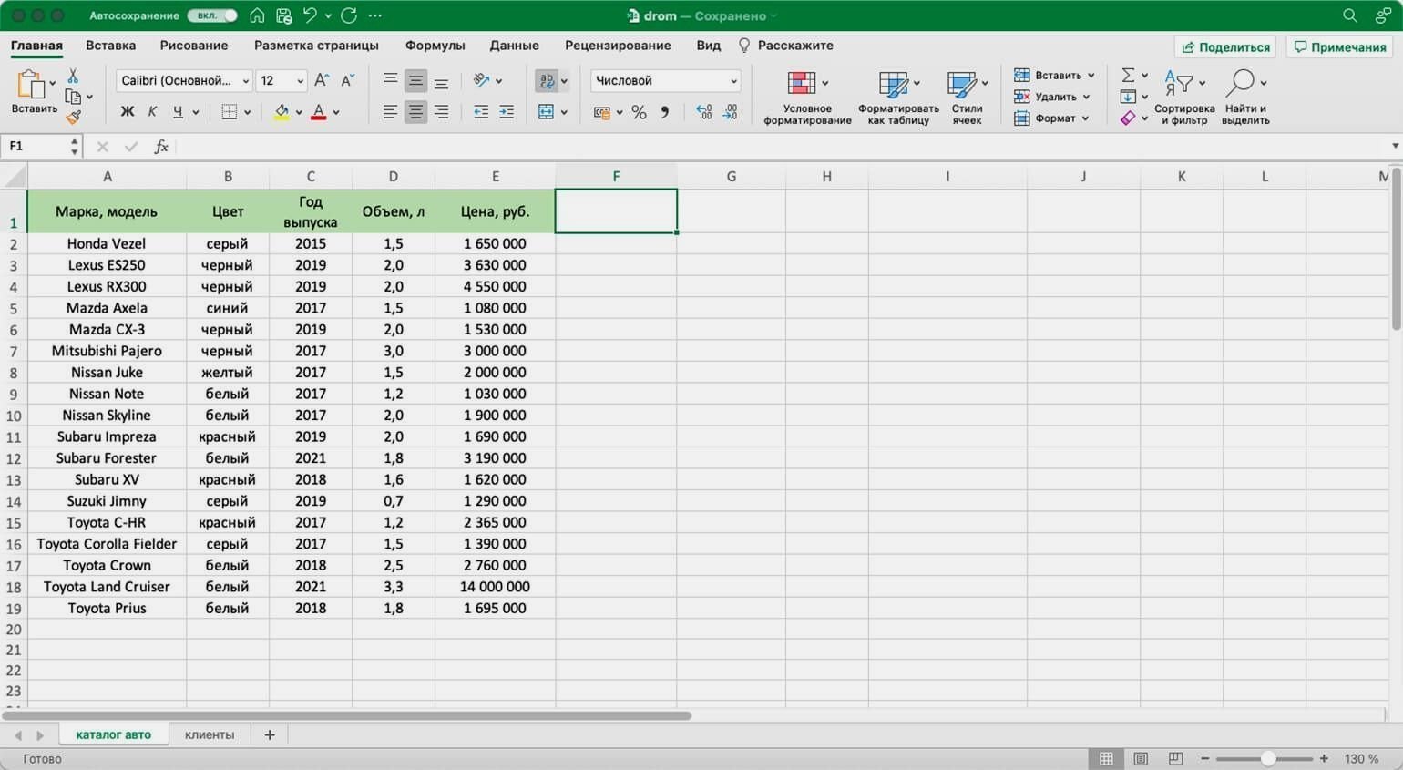
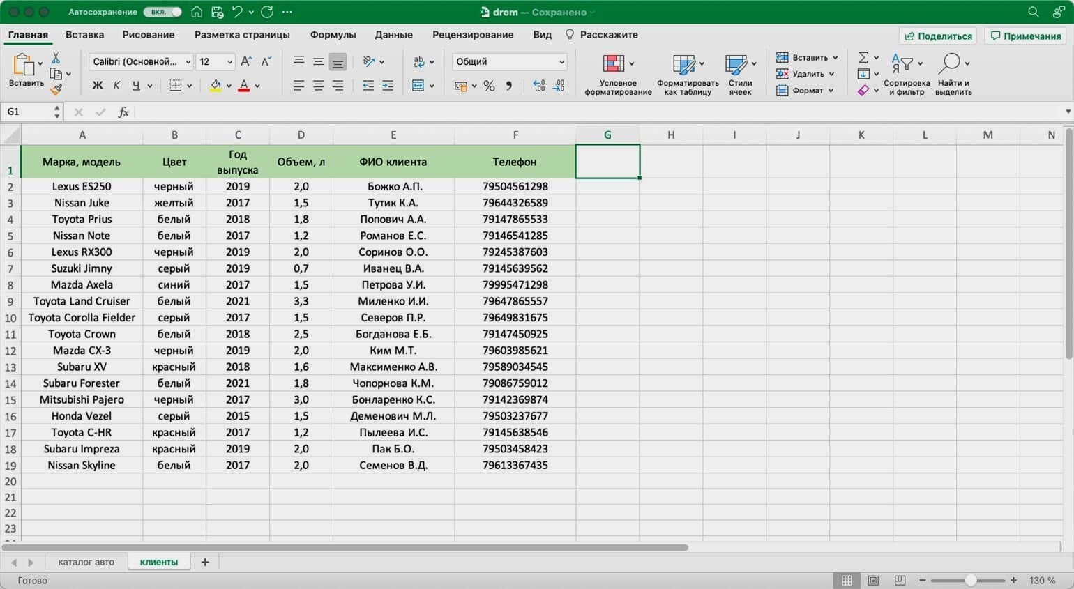
Вам нужно сообщить покупателям, сколько стоят их авто. Перед тем как обзванивать клиентов, нужно объединить данные: добавить во вторую таблицу колонку с ценами из первой.
Просто скопировать и вставить эту колонку не получится. Искать каждое авто вручную и переносить цены — долго.
ВПР автоматически сопоставит названия автомобилей в двух таблицах. Функция скопирует цены из каталога в список забронированных машин. Так напротив каждого клиента будет стоять не только марка автомобиля, но и цена.
Ниже пошагово и со скриншотами разберёмся, как сделать ВПР для этих двух таблиц с данными.

Важно!
ВПР может не работать, если таблицы расположены в разных файлах. Тогда лучше собрать данные в одном файле, на разных листах.
ВПР работает по следующему принципу. Функция просматривает выбранный диапазон первой таблицы вертикально сверху вниз до искомого значения‑идентификатора. Когда видит его, забирает значение напротив него из нужного столбца и копирует во вторую таблицу.
Подробнее о том, как определить все эти значения, поговорим ниже. А пока разберёмся на примере с продажей авто, где найти функцию ВПР в Excel и с чего начать работу.
Сначала нужно построить функцию. Для этого выделяем ячейку, куда функция перенесёт найденное значение.
В нашем случае нужно перенести цены на авто из каталога в список клиентов. Для этого добавим пустой столбец «Цена, руб.» в таблицу с клиентами и выберем ячейку напротив первого клиента.
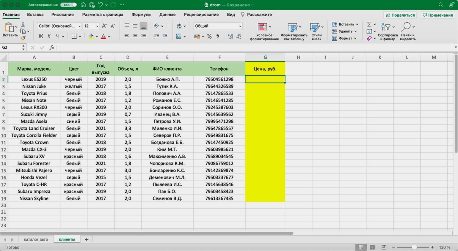
Дальше открываем окно для построения функции ВПР. Есть два способа сделать это. Первый — перейти во вкладку «Формулы» и нажать на «Вставить функцию».
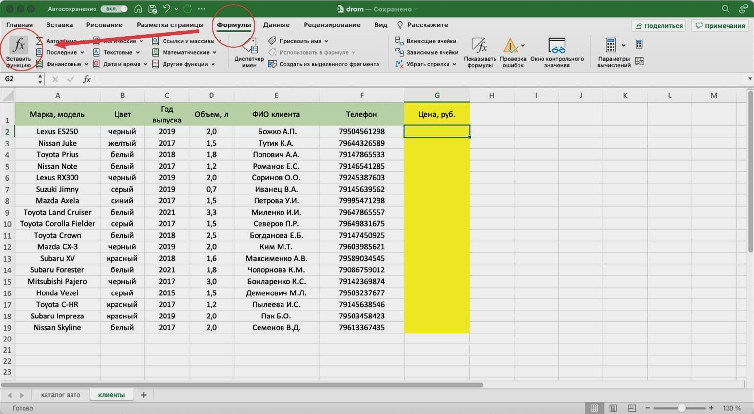
Второй способ — нажать на «fx» в строке ссылок на любой вкладке таблицы.
Справа появляется окно «Построитель формул». В нём через поисковик находим функцию ВПР и нажимаем «Вставить функцию».
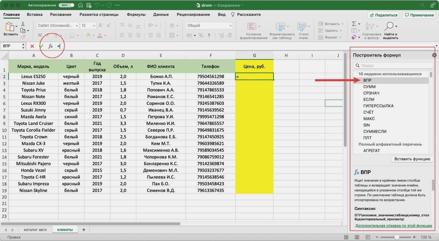
Появляется окно для ввода аргументов функции. Как их заполнять — разбираемся ниже.

Последовательно разберём каждый аргумент: искомое значение, таблица, номер столбца, интервальный просмотр.
Искомое значение — название ячейки с одинаковыми данными для обеих таблиц, по которым функция будет искать данные для переноса. В нашем примере это модель авто. Функция найдёт модель в таблице с каталогом авто, возьмёт оттуда стоимость и перенесёт в таблицу с клиентами.
Порядок действий, чтобы указать значение, выглядит так:
- Ставим курсор в окно «Искомое значение» в построителе формул.
- Выбираем первое значение столбца «Марка, модель» в таблице с клиентами. Это ячейка A2.
Выбранное значение переносится в построитель формул и одновременно появляется в формуле строки ссылок: fx=ВПР(A2).
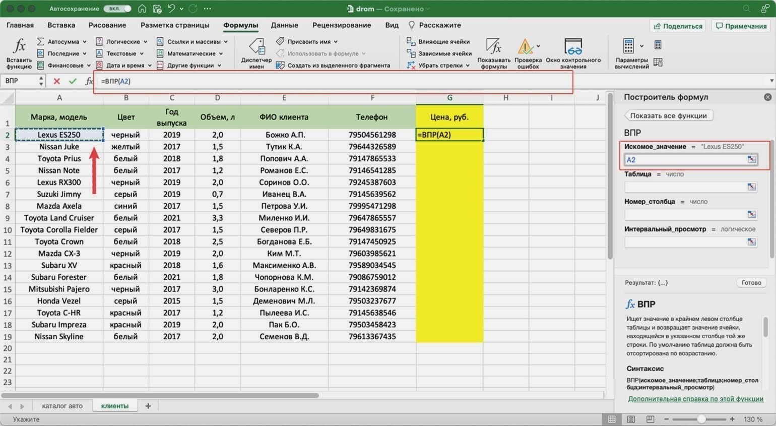
Таблица — это диапазон ячеек, из которого функция будет брать данные для искомого значения. В этот диапазон должны войти столбцы с искомым значением и со значением, которое нужно перенести в первую таблицу.
В нашем случае нужно перенести цены автомобилей. Поэтому в диапазон обязательно нужно включить столбцы «Марка, модель» (искомое значение) и «Цена, руб.» (переносимое значение).
Важно!
Для правильной работы ВПР искомое значение всегда должно находиться в первом столбце диапазона. У нас искомое значение находится в ячейке A2, поэтому диапазон должен начинаться с A.
Порядок действий для указания диапазона:
- Ставим курсор в окно «Таблица» в построителе формул.
- Переходим в таблицу «Каталог авто».
- Выбираем диапазон, в который попадают столбцы «Марка, модель» и «Цена, руб.». Это A2:E19.
- Закрепляем выбранный диапазон. На Windows для этого выбираем значение диапазона в строке ссылок и нажимаем клавишу F4, на macOS — выбираем значение диапазона в строке ссылок и нажимаем клавиши Cmd + T. Закрепить диапазон нужно, чтобы можно было протянуть функцию вниз и она сработала корректно во всех остальных строках.
Выбранный диапазон переносится в построитель формул и одновременно появляется в формуле строки ссылок: fx=ВПР(A2;’каталог авто’!$A$2:$E$19).
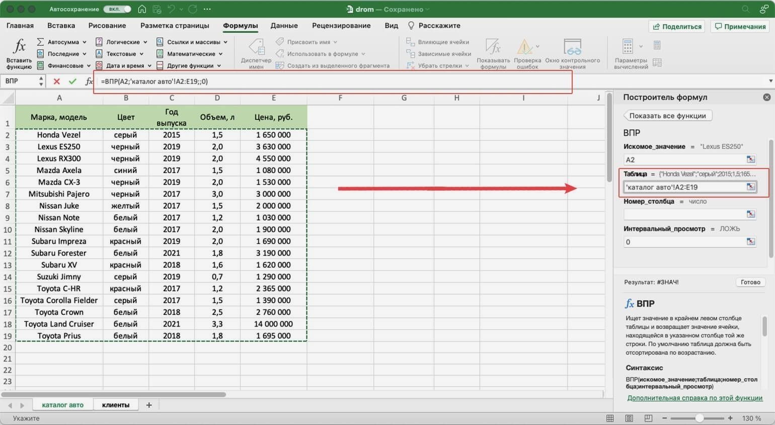
Номер столбца — порядковый номер столбца в первой таблице, в котором находится переносимое значение. Считается по принципу: номер 1 — самый левый столбец, 2 — столбец правее и так далее.
В нашем случае значение для переноса — цена — находится в пятом столбце слева.
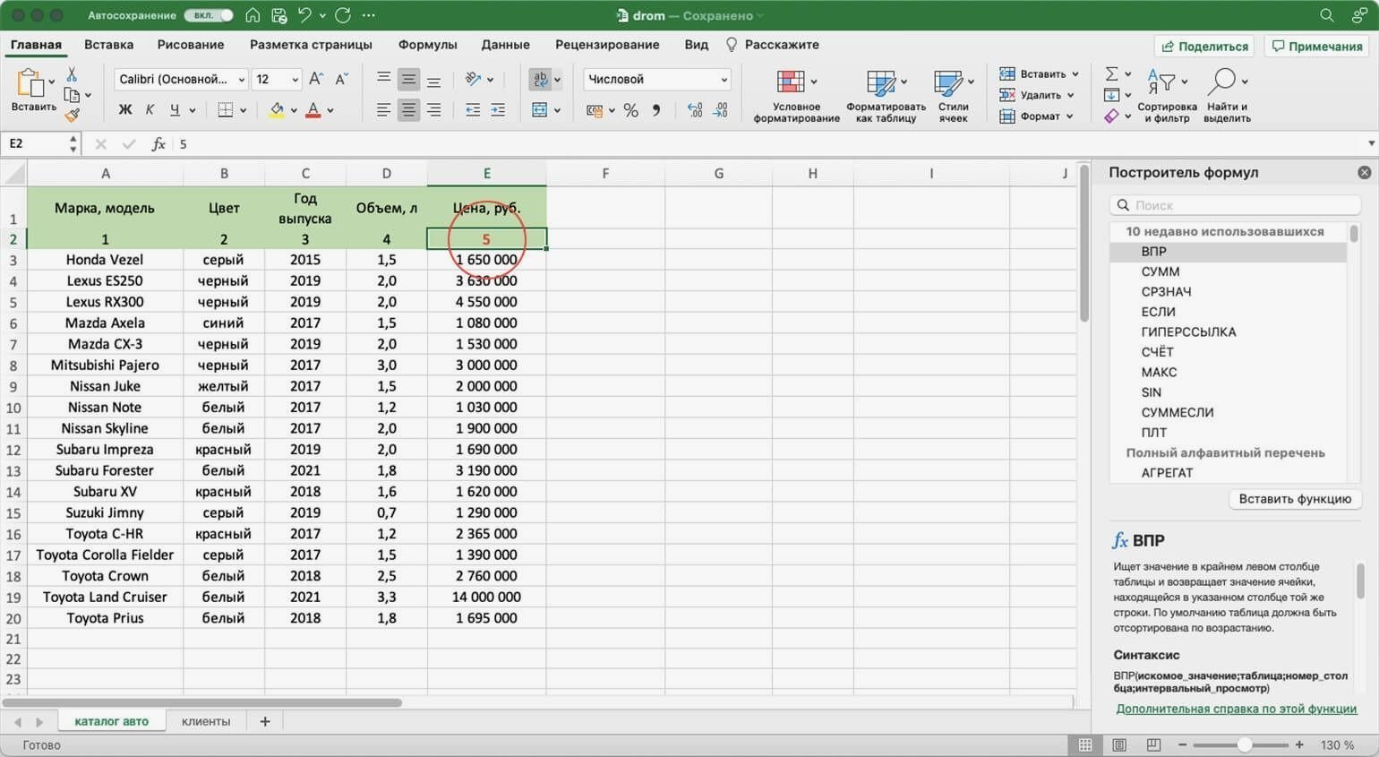
Чтобы задать номер, установите курсор в окно «Номер столбца» в построителе формул и введите значение. В нашем примере это 5. Это значение появится в формуле в строке ссылок: fx=ВПР(A2;’каталог авто’!$A$2:$E$19;5).
Интервальный просмотр — условное значение, которое настроит, насколько точно сработает функция:
- Если нужно точное совпадение при поиске ВПР, вводим 0.
- Если нужно приближённое соответствие при поиске ВПР, вводим 1.
В нашем случае нужно, чтобы функция подтянула точные значения цен авто, поэтому нам подходит первый вариант.
Ставим курсор в окно «Интервальный просмотр» в построителе формул и вводим значение: 0. Одновременно это значение появляется в формуле строки ссылок: fx=ВПР(A2;’каталог авто’!$A$2:$E$19;5;0). Это окончательный вид функции.
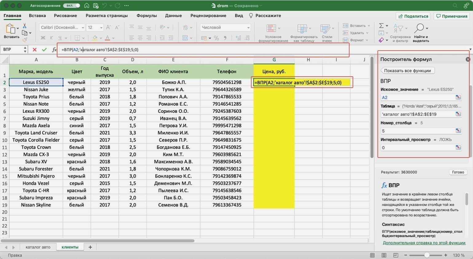
Чтобы получить результат функции, нажимаем кнопку «Готово» в построителе формул. В выбранной ячейке появляется нужное значение. В нашем случае — цена первой модели авто.
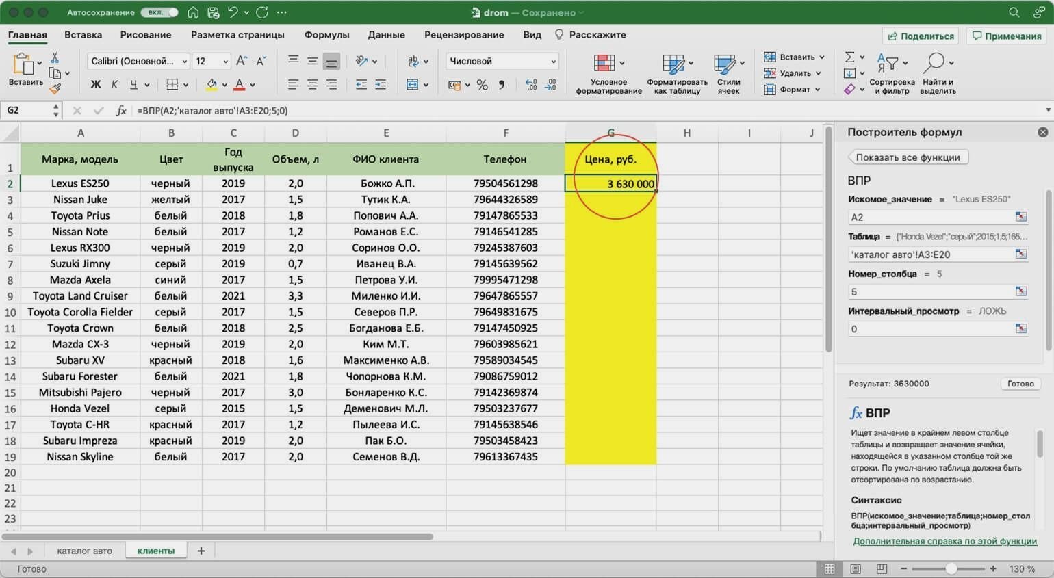
Дальше нужно протянуть это значение вниз до конца таблицы, чтобы функция нашла и перенесла цены всех оставшихся моделей. Для этого мы закрепляли интервал, когда заполняли аргументы.
Получилась таблица с ценами — можно звонить клиентам и сообщать о стоимости авто. Данные перенесены без ошибок, а потратили мы на это несколько минут.
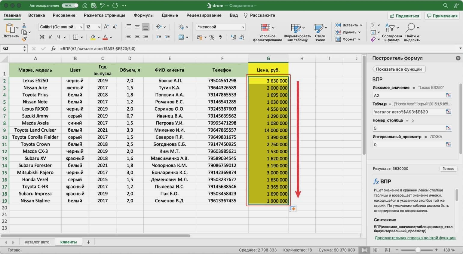
В нашем примере модели автомобилей в таблицах не повторяются, поэтому мы ищем только по одному критерию — названию модели. Но бывают случаи, когда такой поиск не подходит.
Например, у нас несколько одинаковых моделей с разным цветом.
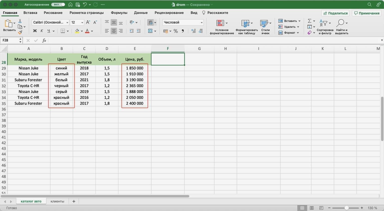
И по традиции есть таблица с клиентами, которые эти модели забронировали.
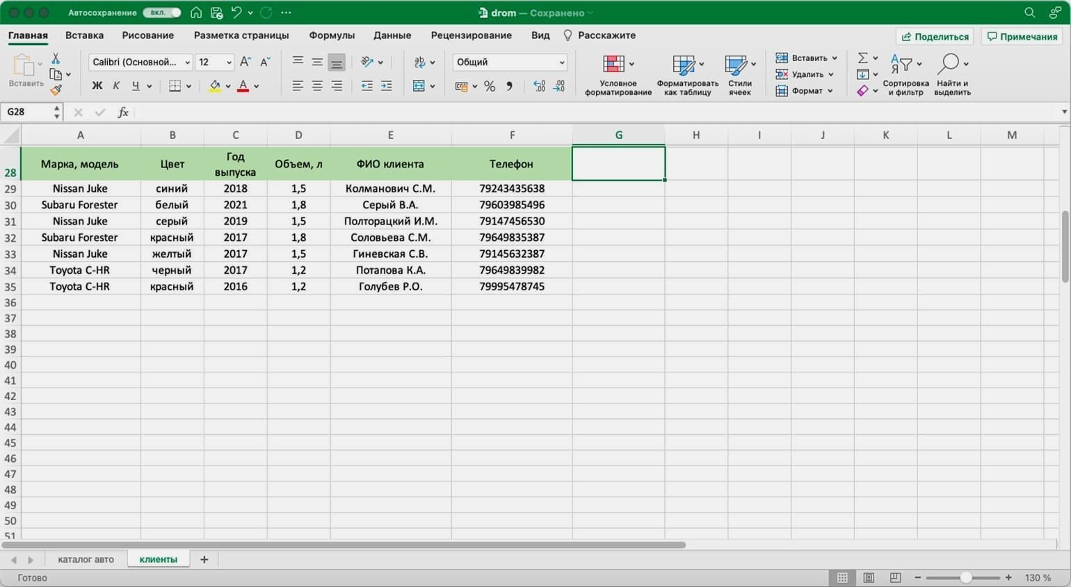
Если идти по классическому пути ВПР, получится такая функция: fx=ВПР(A29;’каталог авто’!$A$29:$E$35;5;0). В таком виде ВПР найдёт первую совпавшую модель и подтянет её стоимость. Параметр цвета не будет учтён.
Соответственно, цены у всех Nissan Juke будут 1 850 000 рублей, у всех Subaru Forester — 3 190 000 рублей, у всех Toyota C-HR — 2 365 000 рублей.
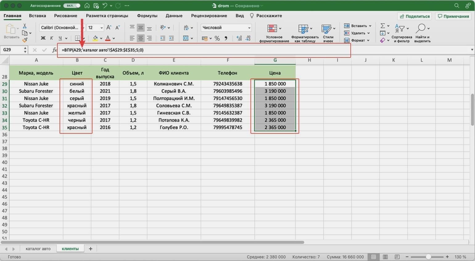
Поэтому в этом варианте нужно искать стоимость авто сразу по двум критериям — модель и цвет. Для этого нужно изменить формулу вручную. В строке ссылок ставим курсор сразу после искомого значения.
Дописываем в формулу фразу ЕСЛИ(‘каталог авто’!$B$29:$B$35=B29, где:
- ‘каталог авто’!$B$29:$B$35 — закреплённый диапазон цвета автомобилей в таблице, откуда нужно перенести данные. Это весь столбец с ценами.
- B29 — искомое значение цвета автомобиля в таблице, куда мы переносим данные. Это первая ячейка в столбце с цветом — дополнительным параметром для поиска.
Итоговая функция такая: fx=ВПР(A29;ЕСЛИ(‘каталог авто’!$B$29:$B$35=B29;’каталог авто’!$A$29:$E$35);5;0). Теперь значения цен переносятся верно.
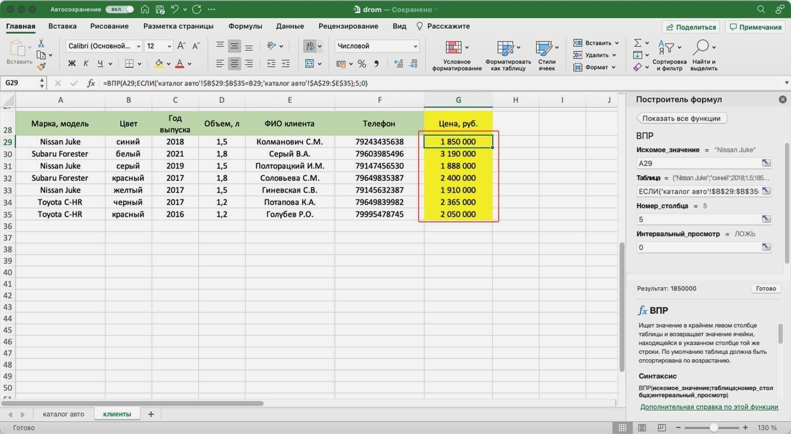
Как использовать ВПР в «Google Таблицах»? В них тоже есть функция Vlookup, но нет окна построителя формул. Поэтому придётся прописывать её вручную. Перечислите через точку с запятой все аргументы и не забудьте зафиксировать диапазон. Для фиксации поставьте перед каждым символом значок доллара. В готовой формуле это будет выглядеть так: =ВПР(A2;’Лист1′!$A$2:$C$5;3;0).

Научитесь: Excel + Google Таблицы с нуля до PRO
Узнать больше
This Excel tutorial explains how to use the VLOOKUP function with syntax and examples.
Description
The VLOOKUP function performs a vertical lookup by searching for a value in the first column of a table and returning the value in the same row in the index_number position.
The VLOOKUP function is a built-in function in Excel that is categorized as a Lookup/Reference Function. It can be used as a worksheet function (WS) in Excel. As a worksheet function, the VLOOKUP function can be entered as part of a formula in a cell of a worksheet.
![]() Subscribe
Subscribe
The VLOOKUP function is actually quite easy to use once you understand how it works! If you want to follow along with this tutorial, download the example spreadsheet.
Download Example
Syntax
The syntax for the VLOOKUP function in Microsoft Excel is:
VLOOKUP( value, table, index_number, [approximate_match] )
Parameters or Arguments
- value
- The value to search for in the first column of the table.
- table
- Two or more columns of data that is sorted in ascending order.
- index_number
- The column number in table from which the matching value must be returned. The first column is 1.
- approximate_match
- Optional. Enter FALSE to find an exact match. Enter TRUE to find an approximate match. If this parameter is omitted, TRUE is the default.
Returns
The VLOOKUP function returns any datatype such as a string, numeric, date, etc.
If you specify FALSE for the approximate_match parameter and no exact match is found, then the VLOOKUP function will return #N/A.
If you specify TRUE for the approximate_match parameter and no exact match is found, then the next smaller value is returned.
If index_number is less than 1, the VLOOKUP function will return #VALUE!.
If index_number is greater than the number of columns in table, the VLOOKUP function will return #REF!.
Example (as Worksheet Function)
Let’s explore how to use VLOOKUP as a worksheet function in Microsoft Excel.
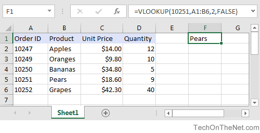
Based on the Excel spreadsheet above, the following VLOOKUP examples would return:
=VLOOKUP(10251, A1:B6, 2, FALSE)
Result: "Pears"   'Returns value in 2nd column

=VLOOKUP(10251, A1:C6, 3, FALSE)
Result: $18.60    'Returns value in 3rd column

=VLOOKUP(10251, A1:D6, 4, FALSE)
Result: 9         'Returns value in 4th column

=VLOOKUP(10248, A1:B6, 2, FALSE)
Result: #N/A      'Returns #N/A error (no exact match)

=VLOOKUP(10248, A1:B6, 2, TRUE)
Result: "Apples"  'Returns an approximate match
Now, let’s look at the example =VLOOKUP(10251, A1:B6, 2, FALSE) that returns a value of «Pears» and take a closer look why.
First Parameter
The first parameter in the VLOOKUP function is the value to search for in the table of data.
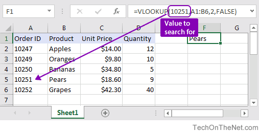
In this example, the first parameter is 10251. This is the value that the VLOOKUP will search for in the first column of the table of data. Because it is a numeric value, you can just enter the number. But if the search value was text, you would need to put it in double quotes, for example:
=VLOOKUP("10251", A1:B6, 2, FALSE)
Second Parameter
The second parameter in the VLOOKUP function is the table or the source of data where the vertical lookup should be performed.
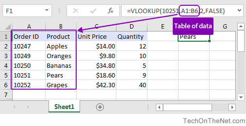
In this example, the second parameter is A1:B6 which gives us two columns to data to use in the vertical lookup — A1:A6 and B1:B6. The first column in the range (A1:A6) is used to search for the Order value of 10251. The second column in the range (B1:B6) contains the value to return which is the Product value.
Third Parameter
The third parameter is the position number in the table where the return data can be found. A value of 1 indicates the first column in the table. The second column is 2, and so on.
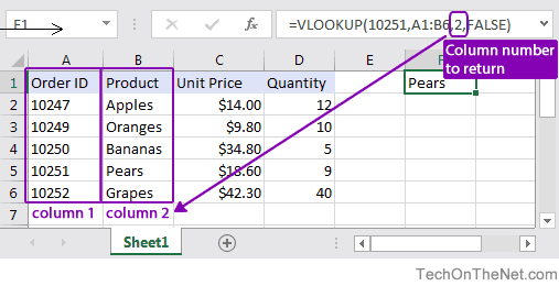
In this example, the third parameter is 2. This means that the second column in the table is where we will find the value to return. Since the table range is set to A1:B6, the return value will be in the second column somewhere in the range B1:B6.
Fourth Parameter
Finally and most importantly is the fourth or last parameter in the VLOOKUP. This parameter determines whether you are looking for an exact match or approximate match.
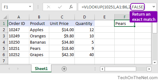
In this example, the fourth parameter is FALSE. A parameter of FALSE means that VLOOKUP is looking for an EXACT match for the value of 10251. A parameter of TRUE means that a «close» match will be returned. Since the VLOOKUP is able to find the value of 10251 in the range A1:A6, it returns the corresponding value from B1:B6 which is Pears.
Exact Match vs. Approximate Match
To find an exact match, use FALSE as the final parameter. To find an approximate match, use TRUE as the final parameter.
Let’s lookup a value that does not exist in our data to demonstrate the importance of this parameter!
Exact Match
Use FALSE to find an exact match:
=VLOOKUP(10248, A1:B6, 2, FALSE)
Result: #N/A
If no exact match is found, #N/A is returned.
Approximate Match
Use TRUE to find an approximate match:
=VLOOKUP(10248, A1:B6, 2, TRUE)
Result: "Apples"
If no match is found, it returns the next smaller value which in this case is «Apples».
VLOOKUP from Another Sheet
You can use the VLOOKUP to lookup a value when the table is on another sheet. Let’s modify our example above and assume that the table is in a different Sheet called Sheet2 in the range A1:B6.
We could rewrite our original example where we lookup the value 10251 as follows:
=VLOOKUP(10251, Sheet2!A1:B6, 2, FALSE)
By preceding the table range with the sheet name and an exclamation mark, we can update our VLOOKUP to reference a table on another sheet.
VLOOKUP from Another Sheet with Spaces in Sheet Name
Let’s throw in one more complication. What happens if your sheet name contains spaces? If there are spaces in the sheet name, you will need to change the formula further.
Let’s assume that the table is on a Sheet called «Test Sheet» in the range A1:B6, now we need to wrap the Sheet name in single quotes as follows:
=VLOOKUP(10251, 'Test Sheet'!A1:B6, 2, FALSE)
By placing the sheet name within single quotes, we can handle a sheet name with spaces in the VLOOKUP function.
VLOOKUP from Another Workbook
You can use the VLOOKUP to lookup a value in another workbook. For example, if you wanted to have the table portion of the VLOOKUP formula be from an external workbook, we could try the following formula:
=VLOOKUP(10251, 'C:[data.xlsx]Sheet1'!$A$1:$B$6, 2, FALSE)
This would look for the value 10251 in the file C:data.xlxs in Sheet 1 where the table data is found in the range $A$1:$B$6.
Why use Absolute Referencing?
Now it is important for us to cover one more mistake that is commonly made. When people use the VLOOKUP function, they commonly use relative referencing for the table range like we did in some of our examples above. This will return the right answer, but what happens when you copy the formula to another cell? The table range will be adjusted by Excel and change relative to where you paste the new formula. Let’s explain further…
So if you had the following formula in cell G1:
=VLOOKUP(10251, A1:B6, 2, FALSE)
And then you copied this formula from cell G1 to cell H2, it would modify the VLOOKUP formula to this:
=VLOOKUP(10251, B2:C7, 2, FALSE)
Since your table is found in the range A1:B6 and not B2:C7, your formula would return erroneous results in cell H2. To ensure that your range is not changed, try referencing your table range using absolute referencing as follows:
=VLOOKUP(10251, $A$1:$B$6, 2, FALSE)
Now if you copy this formula to another cell, your table range will remain $A$1:$B$6.
How to Handle #N/A Errors
Next, let’s look at how to handle instances where the VLOOKUP function does not find a match and returns the #N/A error. In most cases, you don’t want to see #N/A but would rather display a more user-friendly result.
For example, if you had the following formula:
=VLOOKUP(10248, $A$1:$B$6, 2, FALSE)
Instead of displaying #N/A error if you do not find a match, you could return the value «Not Found». To do this, you could modify your VLOOKUP formula as follows:
=IF(ISNA(VLOOKUP(10248, $A$1:$B$6, 2, FALSE)), "Not Found", VLOOKUP(10248, $A$1:$B$6, 2, FALSE))
OR
=IFERROR(VLOOKUP(10248, $A$1:$B$6, 2, FALSE), "Not Found")
OR
=IFNA(VLOOKUP(10248, $A$1:$B$6, 2, FALSE), "Not Found")
These formulas use the ISNA, IFERROR and IFNA functions to return «Not Found» if a match is not found by the VLOOKUP function.
This is a great way to spruce up your spreadsheet so that you don’t see traditional Excel errors.
Frequently Asked Questions
If you want to find out what others have asked about the VLOOKUP function, go to our Frequently Asked Questions.
Frequently Asked Questions