Поиск значения в таблице (диапазоне, массиве) по значению в первом столбце таблицы с помощью метода VBA Excel WorksheetFunction.VLookup. Синтаксис, параметры, примеры.
WorksheetFunction.VLookup – это метод VBA Excel, который ищет значение в крайнем левом столбце таблицы (диапазона, двумерного массива) и возвращает значение ячейки (элемента массива), находящейся в указанном столбце той же строки. Метод соответствует функции рабочего листа =ВПР (вертикальный просмотр).
Синтаксис
Синтаксис метода WorksheetFunction.VLookup в VBA Excel:
|
WorksheetFunction.VLookup(Arg1, Arg2, Arg3, Arg4) |
Параметры
Описание параметров метода WorksheetFunction.VLookup:
| Параметр | Описание |
|---|---|
| Arg1 (Lookup_value) | Обязательный параметр. Значение, которое необходимо найти в первом столбце таблицы. |
| Arg2 (Table_array) | Обязательный параметр. Таблица с двумя или более столбцами данных. Используется ссылка на диапазон, имя диапазона или массив. |
| Arg3 (Col_index_num) | Обязательный параметр. Номер столбца, значение из которого возвращается. |
| Arg4 (Range_lookup) | Необязательный параметр. Логическое значение, указывающее, должен ли метод VLookup искать точное совпадение или приблизительное. |
Значения параметра Arg4 (Range_lookup), задающие точность сопоставления:
| Значение | Точность сопоставления |
|---|---|
| True | Значение по умолчанию. Метод WorksheetFunction.VLookup находит точное или приблизительное совпадение Arg1 со значением в первом столбце. Если точное совпадение не найдено, используется самое большое значение, меньшее Arg1. Значения в первом столбце таблицы должны быть отсортированы по возрастанию. |
| False | Метод WorksheetFunction.VLookup находит только точное совпадение. Сортировка значений первого столбца таблицы не требуется. Если точное совпадение не найдено, генерируется ошибка. |
Если значение параметра Arg1 является текстом, а Arg4=False, тогда в строке Arg1 можно использовать знаки подстановки (спецсимволы): знак вопроса (?) и звездочку (*). Знак вопроса заменяет один любой символ, а звездочка соответствует любой последовательности символов. Чтобы знак вопроса (?) и звездочка (*) обозначали сами себя, перед ними указывается тильда (~).
Примеры
Примеры обкатывались на следующей таблице:
Поиск значения в таблице
|
Sub Primer1() Dim x x = «Смартфон: « & WorksheetFunction.VLookup(7, Range(«A2:D11»), 2, False) MsgBox x End Sub |
Результат работы кода:
Поиск значения в массиве
|
Sub Primer2() Dim x, y x = Range(«A2:D11») y = «Смартфон: « & WorksheetFunction.VLookup(8, x, 2, False) & vbNewLine _ & «Разрешение экрана: « & WorksheetFunction.VLookup(8, x, 3, False) & vbNewLine _ & «Емкость аккумулятора: « & WorksheetFunction.VLookup(8, x, 4, False) & » мАч» MsgBox y End Sub |
Результат работы кода:
Да, здесь можно немного улучшить структуру кода, применив оператор With...End With:
|
Sub Primer3() Dim x, y x = Range(«A2:D11») With WorksheetFunction y = «Смартфон: « & .VLookup(8, x, 2, False) & vbNewLine _ & «Разрешение экрана: « & .VLookup(8, x, 3, False) & vbNewLine _ & «Емкость аккумулятора: « & .VLookup(8, x, 4, False) & » мАч» End With MsgBox y End Sub |
“Constant effort and frequent mistakes are the stepping stones to genius” – Elbert Hubbard
A Quick Guide to the VBA VLookup
| Parameters | Type |
|---|---|
| Lookup value | The value you are searching for |
| Table array | The range you are searching through |
| Column index | The column number of the value to return. |
| Range look up | Optional — set to False for exact match only. |
Introduction
The VLookup function can be a useful Excel function. Even though it is straightforward to use can often be confusing when used in VBA. In this post, I am going to show how anyone can easily use the VLookup function. I’ll also cover the pitfalls and how to avoid them. Of course, no post would be complete without a ton of examples that you can try for yourself.
If you are not familiar with VLookup in Excel then this page provides a great introduction.
Notes: I use the Underscore character(_) in the code examples. In VBA this allows you to split a line over multiple lines e.g.
' One line
sResult = Application.VLookup("Apricot", Sheet1.Range("A10:B10000"), 1)
' Split up with underscore
sResult = Application.VLookup( _
    "Apricot", Sheet1.Range("A10:B10000"), 1)
A Simple VBA VLookup example
Note: The variable shData in the examples refers to the worksheet by the code name. You can replace this with the code name of the worksheet you are using.
Take a look at the following data:
Use this code to generate this data on any worksheet:
' Use this sub to generate the data
' https://excelmacromastery.com
Sub GenerateData()

    ' Change the sheet name as required
    With ThisWorkbook.Worksheets("Sheet1")

        .Range("A1").CurrentRegion.ClearContents
        .Range("A1:A7").Value = WorksheetFunction.Transpose(Array("Fruit", "Apple", "Apricot", "Orange", "Peach", "Pair", "Plum"))
        .Range("B1:B7").Value = WorksheetFunction.Transpose(Array("Price", 1.56, 2.33, 1.45, 2.28, 1.67, 1.22))

    End With

End Sub
The code below will return the price for the Pear i.e. 1.45
' https://excelmacromastery.com/
Sub SimpleVLookup()

    Dim sRes As String
    sRes = Application.VLookup("Pear",shData.Range("A2:B7"),2)

    ' This will print 1.67 to the Immediate Window(Ctrl + G)
    Debug.Print sRes

End Sub
The code looks for the text Pear in the range A2:B7. When it finds the text it returns a value from the same row as the text. The value in determined by the column number argument. We used 2 in this example.
Let’s look at some more examples and results
' Returns 1.45
sRes = Application.VLookup("Orange",shData.Range("A2:B7"),2)

' Returns 1.56
sRes = Application.VLookup("Apple",shData.Range("A2:B7"),2)

' Returns 1.22
sRes = Application.VLookup("Plum",shData.Range("A2:B7"),2)

' Returns Orange as column is 1
sRes = Application.VLookup("Orange",shData.Range("A2:B7"),1)

' Returns Apple as column is 1
sRes = Application.VLookup("Apple",shData.Range("A2:B7"),1)

' Returns Plum as column is 1
sRes = Application.VLookup("Plum",shData.Range("A2:B7"),1)
The Parameters
In this section we will look at the four parameters. These are
- lookup_value – The value to look up. It must be in the first column of the range.
- table_array – This is the range to search. This can also be a VBA array although it very slow using this.
- col_index_num – This contains the column number of the return value. Starts at column number one.
- range_lookup(optional) – Use True(default) to find closest match. Use False to find exact match. Using True assumes that the first columnis sorted alphabetically or numerically.
We will look at these parameters individually starting with the lookup_value parameter.
Parameter 1: lookup_value
This is the value that you are looking up. It must be in the first column of the Range. If you are using the range C4:X10 then the lookup value must be in column C. If you are using the range Z1:AB5 then the lookup value must be in column Z.
The type of value you search for will normally be a string as this example shows
' https://excelmacromastery.com/
Sub StringVLookup()

    Dim sFruit As String
    sFruit = "Plum"

    Dim sRes As Variant
    sRes = Application.VLookup( _
                       sFruit, shData.Range("A2:B7"), 2, False)

End Sub
We can also search for a number but you have to be careful here:
- If the number is stored as text then the search value must be a string.
- If the number is stored as a number then the search value must be a number.
For example in this data we have the lookup column stored as numbers
In this case, the lookup value must be a Long or you will get an error message.
' https://excelmacromastery.com/
Sub NumberVLookup()

    Dim num As Long
    num = 7

    Dim sRes As Variant
    sRes = Application.VLookup( _
                  num, shData.Range("F2:G7"), 2, True)

    Debug.Print sRes

End Sub
You can also use the Double data type if you are looking up a decimal value. As in the case of an integer it must be stored as a number if you want to use Double.
Using VLookup on a Date Type
Using a Date type is a tricky business. VBA has a Date data type but the worksheet does not.
So the date type needs to be converted to a Long as the following examples show
theDate = CLng(#1/14/2017#)

theDate = CLng(CDate("1/14/2017"))

theDate = CLng(shData.Range("H10"))
You can then use it as normal in the VLookup function when the search column contains dates
' https://excelmacromastery.com/
Sub DateVLookup()

    Dim theDate As Long
    theDate = CLng(#1/14/2017#)

    Dim sRes As Variant
    sRes = Application.VLookup( _
                 theDate, shData.Range("I2:J7"), 2, False)

    Debug.Print sRes

End Sub
Parameter 2: table_array
This parameter refers to the range of the data we are looking up. You will normally use a range for this as we have seen in the examples so far.
If you are using a worksheet table you can use the range of the table.
' https://excelmacromastery.com/
Sub SimpleVLookupTable()

    Dim sRes As Variant

    ' Get the table
    Dim table As ListObject
    Set table = shData.ListObjects("Table1")

    ' Use the table for the table_array parameter
    sRes = Application.VLookup( _
                  "Plum", table.Range, 2, False)

    Debug.Print sRes

End Sub
You can also use a VBA array with VLookup but this tends to be very slow.
Parameter 3: col_index-num
This parameter refers to the column which contains the value you want to return. Column 1 is the leftmost column of the table_array.
If the column number is greater than the number of columns in the range you will get an error. See The VLookup Error Types section below.
© BigStockPhoto.com
Parameter 4: range_lookup
This is an optional parameter. If it is not used then it takes True as the default value.
False means that an exact match must be found.
True means that an approximate match will be returned. The first column must be ordered numerically or alphabetically for this to work correctly.
Let’s look at the sample data again
The following code shows some examples of how this parameter works:
' https://excelmacromastery.com/
Sub SimpleVLookup()

    Dim rg As Range
    Set rg = shData.Range("A2:B7")

    Dim sRes As Variant

    ' Stops at Orange - the last item before a P item
    sRes = Application.VLookup("P", rg, 2, True)

    ' Stops at Orange - the last item before a Pea item
    sRes = Application.VLookup("Pea", rg, 2, True)

    ' Stops at Peach - the last item before a Pead item
    sRes = Application.VLookup("Pead", rg, 2, True)

    ' Error - no exact match found
    sRes = Application.VLookup("Pea", rg, 2, False)


End Sub
Dealing with Errors
© BigStockPhoto.com
We can use VLookup in two ways in VBA. With Application or with WorksheetFunction
Application.WorksheetFunction.VLookup

Application.VLookup
The difference between them is how we handle errors. Let’s look at each of these in turn.
Using WorksheetFunction
Using WorksheetFunction.VLookup requires us to use On Error to trap the error. We can then check the error number Err.Number to see if the value is valid.
' https://excelmacromastery.com/
Sub UseWorksheetFunction()

    Dim sRes As Variant

    ' Turn on error trapping
    On Error Resume Next
    Err.Clear

    sRes = Application.WorksheetFunction.VLookup _
                ("Plum", shData.Range("A2:B7"), 2, False)

    ' Check if value found
    If Err.Number = 0 Then
        Debug.Print "Found item. The value is " & sRes
    Else
        Debug.Print "Could not find value: " & "Plum"
    End If

End Sub
Using Application
Using Application.VLookup we can simply check the return value to see if there was an error
' https://excelmacromastery.com/
Sub UsingApplication()

    Dim sRes As Variant

    sRes = Application.VLookup _
                ("Plum", shData.Range("A2:B7"), 2, False)

    ' Check if value found
    If IsError(sRes) = False Then
        Debug.Print "Found item. The value is " & sRes
    Else
        Debug.Print "Could not find value: " & "Plum"
    End If

End Sub
VLookup Error Types
The following table shows a list of the Excel cell error numbers and what they mean. These are the error numbers we get when we use Application.VLookup. This is taken from this MSDN Page
| Constant | Error number | Cell error value |
|---|---|---|
| xlErrDiv0 | 2007 | #DIV/0 |
| xlErrNA | 2042 | #N/A |
| xlErrName | 2029 | #NAME? |
| xlErrNull | 2000 | #NULL! |
| xlErrNum | 2036 | #NUM! |
| xlErrRef | 2023 | #REF! |
| xlErrValue | 2015 | #VALUE! |
Errors and Causes
The following table shows some common errors you may encounter with VLookup. If you’re having trouble with a particular VLookup error then it is a good idea to try it in Excel first.
| Error | Cell | Possible causes |
|---|---|---|
| Error 2015 | #VALUE! | The column number is less than one. |
| Error 2015 | #VALUE! | You used a string instead of a range for the table_array parameter. |
| Error 2023 | #REF! | The column number is greater than the number of columns. |
| Error 2042 | #N/A | The value is not found. See possible causes below. |
If you cannot find the value then check the following:
- Ensure the Table/Range is correct.
- Ensure the Table/Range does not include the header(VBA will think list is unsorted).
- Ensure the Table/Range is using the correct worksheet.
- If searching for a number use a long or double data type in the lookup_value parameter. See lookup_value section above
- If searching for a number stored as text use a string data type in the lookup_value parameter.
- If searching for a date convert it to a long(see Date Type above) in the lookup_value parameter.
If you are getting the wrong value then check the following:
- If the range_lookup parameter is True or not used, then ensure the first column is sorted alphabetically or numerically (see range_lookup above)
VBA VLookup Speed
Sometimes you may need to perform a large number of lookups. In these cases, VLookup could be too slow. The VBA Dictionary is faster when dealing with a large number of lookups. The following code shows an example of using the Dictionary.
' https://excelmacromastery.com/
Sub UseDictionary()

    ' Get the range of values
    Dim rg As Range
    Set rg = shData.Range("M1:N20000")

    ' Create the dictionary
    Dim dict As Object
    Set dict = CreateObject("Scripting.Dictionary")

    ' Fill the dictionary
    Dim cell As Range
    For Each cell In rg
        dict(cell.Value) = cell.Offset(0, 1).Value
    Next

    ' Perform the Lookups
    For Each cell In rg
        Debug.Print dict(cell.Value)
    Next

End Sub
What’s Next?
Free VBA Tutorial If you are new to VBA or you want to sharpen your existing VBA skills then why not try out the The Ultimate VBA Tutorial.
Related Training: Get full access to the Excel VBA training webinars and all the tutorials.
(NOTE: Planning to build or manage a VBA Application? Learn how to build 10 Excel VBA applications from scratch.)
In my earlier post, I had written about VLOOKUP in Excel. It was a massive post of around 2500 words, it explains most of the things about the vertical lookup function in excel. Today’s post is an extension to that post and here we will understand how to apply a VLOOKUP in VBA.
If you haven’t read that post then I would strongly recommend you read that post before going any further. [Read Here]
Assuming that you have basic knowledge of the VLOOKUP function we will move further.
Note: To perform these programs yourself, you may need to enable macros in excel. Read this post to know how to do this.
Syntax of VBA VLOOKUP
You can use VLookUp in macros by following any of the below ways:
Application.VLOOKUP(lookup_value, table_array, column_index, range_lookup)
Or
Application.WorksheetFunction.VLOOKUP(lookup_value, table_array, column_index, range_lookup)
Note: If you are searching for something similar to the VLOOKUP function for Access then probably you should use DLOOKUP.
5 Examples of Using VLOOKUP in VBA
Now let’s move to some practical examples of using VLookUp in VBA codes.
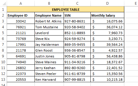
Example 1
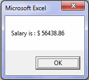
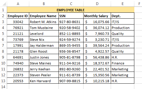
Using VLookUp find the monthly salary of “Justin Jones” from the below table. Display the salary using a dialog box.
Below is the code for this:
Sub FINDSAL()
Dim E_name As String
E_name = "Justin Jones"
Sal = Application.WorksheetFunction.VLookup(E_name, Sheet1.Range("B3:D13"), 3, False)
MsgBox "Salary is : $ " & Sal
End Sub
Explanation: In this code, we have used a variable ‘E_name’ to store the employee name whose salary is to be fetched. After this, we have simply supplied the employee name and other required arguments to the VLOOKUP and it returns the salary of the corresponding Employee.
Example 2
Now make the above program a little customizable by accepting the Employee name from the user. If the user enters any Employee name that is not present in the table then the program should be able to convey this clearly to the user.
To accomplish this we can use the below code:
Sub FINDSAL()
On Error GoTo MyErrorHandler:
Dim E_name As String
E_name = InputBox("Enter the Employee Name :")
If Len(E_name) > 0 Then
 Sal = Application.WorksheetFunction.VLookup(E_name, Sheet1.Range("B3:D13"), 3, False)
 MsgBox "Salary is : $ " & Sal
Else
 MsgBox ("You entered an invalid value")
End If
Exit Sub
MyErrorHandler:
If Err.Number = 1004 Then
 MsgBox "Employee Not Present in the table."
End If
End Sub
Explanation: In this code, we are accepting the user input using an InputBox function. If the Employee name entered by the user is found, then VLookUp returns its corresponding salary. However, if the employee name is not present in the table then VLOOKUP throws a “1004 Error”.
And, we have created an error handler to catch such cases for conveying the user that entered employee name doesn’t exist.
Example 3
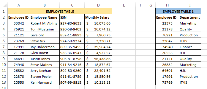
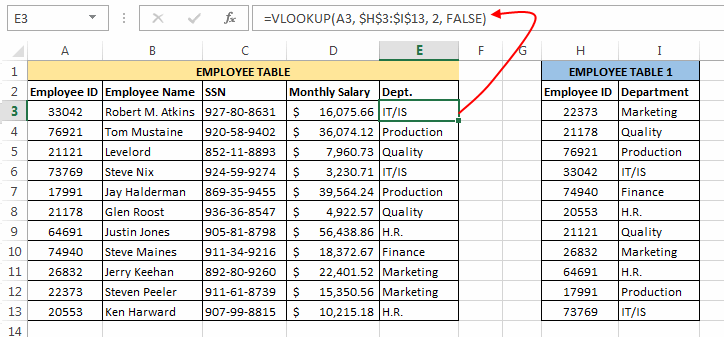
In this example we will try to write a code that adds the Department field from the Employee Table 1 to our old Employee Table.
As you can see that in both these tables there is only one common column i.e. Employee_ID. So, in this case, we will have to apply the VLookUp based on the Employee ID.
Below is the code to do this:
Sub ADDCLM()
On Error Resume Next
Dim Dept_Row As Long
Dim Dept_Clm As Long
Table1 = Sheet1.Range("A3:A13") ' Employee_ID Column from Employee table
Table2 = Sheet1.Range("H3:I13") ' Range of Employee Table 1
Dept_Row = Sheet1.Range("E3").Row ' Change E3 with the cell from where you need to start populating the Department
Dept_Clm = Sheet1.Range("E3").Column
For Each cl In Table1
 Sheet1.Cells(Dept_Row, Dept_Clm) = Application.WorksheetFunction.VLookup(cl, Table2, 2, False)
 Dept_Row = Dept_Row + 1
Next cl
MsgBox "Done"
End Sub
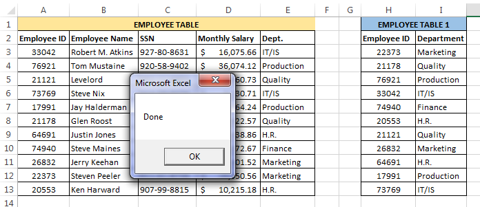
Explanation: This code takes each ‘lookup_value’ from the Employee ID field (one at a time), looks up its corresponding Department, and then populates the corresponding department value at the appropriate place.
Please note that in this code we have just pasted the result of the VLOOKUP formula, and not the VLookUp formula itself (Refer Example 5).
Example 4
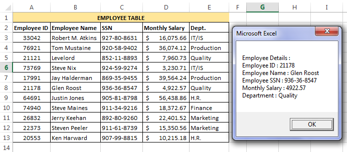
In this example we will try to write a code that displays all the details of an employee from the Employee table (as shown below) when its Employee ID is entered.
Below is the code that can accomplish this:
Sub FETCH_EMP_DETAILS()
On Error GoTo MyErrorHandler:
Dim E_id As Long
E_id = InputBox("Enter the Employee ID :")
Det = "Employee ID : " & Application.WorksheetFunction.VLookup(E_id, Sheet1.Range("A3:E13"), 1, False)
Det = Det & vbNewLine & "Employee Name : " & Application.WorksheetFunction.VLookup(E_id, Sheet1.Range("A3:E13"), 2, False)
Det = Det & vbNewLine & "Employee SSN : " & Application.WorksheetFunction.VLookup(E_id, Sheet1.Range("A3:E13"), 3, False)
Det = Det & vbNewLine & "Monthly Salary : " & Application.WorksheetFunction.VLookup(E_id, Sheet1.Range("A3:E13"), 4, False)
Det = Det & vbNewLine & "Department : " & Application.WorksheetFunction.VLookup(E_id, Sheet1.Range("A3:E13"), 5, False)
MsgBox "Employee Details : " & vbNewLine & Det
Exit Sub
MyErrorHandler:
If Err.Number = 1004 Then
 MsgBox "Employee Not Present in the table."
ElseIf Err.Number = 13 Then
 MsgBox "You have entered an invalid value."
End If
End Sub
Explanation: In this example, we have asked the user to enter the Employee Id and then we have used multiple VLookUp Statements and concatenated their outputs to show all the details in a single message box.
Example 5
Redo example 3 but this time paste the whole VLookUp formula instead of pasting only the result.
Below is the code for doing this:
Sub ADDCLM()
On Error Resume Next
Dim Dept_Row As Long
Dim Dept_Clm As Long
ctr = 0
Table1 = Sheet1.Range("A3:A13") ' Employee_ID Column from Employee table
Table2 = Sheet1.Range("H3:I13") ' Range of Employee Table 1
Dept_Row = Sheet1.Range("E3").Row ' Change E3 with the cell from where you need to start populating the Department
Dept_Clm = Sheet1.Range("E3").Column
For Each cl In Table1
 Sheet1.Cells(Dept_Row, Dept_Clm).FormulaR1C1 = "=VLOOKUP(RC[-4], R3C8:R13C9, 2, False)"
 Dept_Row = Dept_Row + 1
 ctr = ctr + 1
Next cl
MsgBox "Done"
End Sub
Explanation: This code is very similar to the one that we have discussed in Example 3, the only difference between these formulas is that here we are copying the VLookUp formula directly in the cells.
In this code, we have applied the VLOOKUP in R1C1 form. So, the formula =VLOOKUP(RC[-4], R3C8:R13C9, 2, False) means =VLOOKUP(<4 cells to the left of current cell>, <Range of Employee Table 1>, <column to be fetched>, <exact match>).
One thing that is worth noting here is: the square brackets ( [ ] ) in your R1C1 formula indicate that you are specifying a relative range. If you want to specify an absolute range, you need to specify the R1C1 cells without brackets; e.g. R3C8:R13C9.
So, this was all about VBA VLOOKUP .
In this Article
- VLOOKUP
- Application.WorksheetFunction.VLookup
- Application.VLookup vs Application.WokrsheetFunction.VLookup
- WorksheetFunction.XLOOKUP
This article will demonstrate how to use the VLOOKUP and XLOOKUP functions in VBA.
The VLOOKUP and XLOOKUP functions in Excel are extremely useful. They can also be used in VBA Coding.
VLOOKUP
There are two ways to call the VLOOKUP Function in VBA:
- Application.WorksheetFunction.Vlookup
- Application.Vlookup
The two methods worked identically, except for how they handle errors.
Application.WorksheetFunction.VLookup
This example will demonstrate the first method.
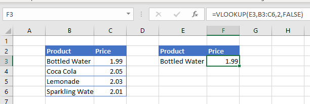
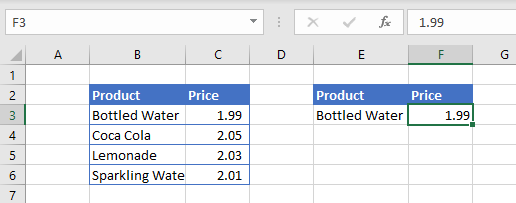
Here we’ve created a VLOOKUP formula in Excel that we will replicate in VBA:
Sub LookupPrice()
   ActiveCell = Application.WorksheetFunction.VLookup(Range("E3"), Range("B2:C6"), 2, False)
End Sub
This will result in the following:
Note that the actual result was written to cell F3 instead of the formula!
If we wish to return a formula to Excel instead of a value, write the VLOOKUP into a formula:
Sub LookupPrice()
   ActiveCell = "=VLOOKUP(E3,B2:C6,2,FALSE)"
End Sub
Or you can write the formula to a cell using R1C1 notation, which creates a formula with relative references that can be used over a range of cells:
Sub LookupPrice()
  ActiveCell = "=VLOOKUP(RC[-1],RC[-4]:R[3]C[-3],2,FALSE)"
End Sub
You can also use variables to define the VLOOKUP inputs:
Sub LookupPrice()
 Dim strProduct As String
 Dim rng As Range
 strProduct = Range("E3")
 Set rng = Range("B2:C6")
 ActiveCell = Application.WorksheetFunction.VLookup(strProduct, rng, 2, False)
End Sub
Of course, instead of writing the results of the function to a cell, you can write the results to a variable:
Sub LookupPrice()
  Dim strProduct As String
  Dim rng As Range
  Dim strResult as String

  strProduct = Range("E3")
  Set rng = Range("B2:C6")
  strResult = Application.WorksheetFunction.VLookup(strProduct, rng, 2, False)
End Sub
Application.VLookup vs Application.WokrsheetFunction.VLookup
In the examples above, we can use either of the methods and they will return the same result. However what if we were looking up a Product that doesn’t exist – what result would this return? Each function would return a very different result.
Normally when using VLOOKUP in Excel, if the Lookup does not find the correct answer, it returns #N/A back to the cell. However, if we use the example above and look for a product that does not exist, we will end up with a VBA Error.
We can trap for this error in our code and return a more user friendly message when the item we are looking for is not found.
Sub LookupPrice()
  On Error GoTo eh
  ActiveCell = Application.WorksheetFunction.VLookup(Range("E3"), Range("B2:C6"), 2, False)
  Exit Sub
eh:
  MsgBox "Product not found - please try another product"
End Sub
Alternatively, we can amend our VBA code to use Application.Vlookup instead of Application.WorksheetFunction.VLookup.
Sub LookupPrice()
  ActiveCell = Application.VLookup(Range("E3"), Range("B2:C6"), 2, False)
End Sub
When we do this, the #N/A that we have come to expect when a lookup value is not found, is returned to the cell.
WorksheetFunction.XLOOKUP
The XLOOKUP function has been designed to replace the VLOOKUP and HLOOKUP functions in Excel. It is only available to Office 365 so using this function is quite restrictive is some of your users are using older versions of Excel.
It works in much the same ways in VBA as the VLOOKUP function.
Sub LookupPriceV()
   ActiveCell = Application.WorksheetFunction.XLookup(Range("E3"), Range("B2:B6"), Range("C2:C6"))
End Sub
OR
Sub LookupPriceV()
   ActiveCell = Application.XLookup(Range("E3"), Range("B2:B6"), Range("C2:C6"))
End Sub
Once again, if we wish to use variables, we can write the following code
Sub LookupPriceV()
   Dim strProduct As String
   Dim rngProduct As Range
   Dim rngPrice As Range
   strProduct = Range("E3")
   Set rngProduct = Range("B2:B6")
   Set rngPrice = Range("C2:C6")
   ActiveCell = Application.WorksheetFunction.XLookup(strProduct, rngProduct, rngPrice)
End Sub
If we wish to return a formula to Excel instead of a value, we would need to write the formula into Excel with the VBA code.
Sub LookupPrice()
   ActiveCell = "=XLOOKUP(E3,B3:B6,C3:C6)"
End Sub
Or you can write the formula to a cell using R1C1 notation.
Sub LookupPrice()
  ActiveCell.Formula2R1C1 = "=XLOOKUP(RC[-1],RC[-4]:R[3]C[-4],RC[-3]:R[3]C[-3])"
End Sub
One of the major advantages of using XLOOKUP vs VLOOKUP is the ability to lookup a range of columns, and return the value in each column.
Lets look at the following example:
We have created the formula in cell H3 where it is looking up the values in the range C2:E6. Due to the fact that these are multiple columns, it will automatically populate columns I and J with the matching results found. The formula SPILLS over into columns I and J without us having to use CTRL+SHIFT for an array formula – this ability for the formula to SPILL across is one of the new additions for Excel 365.
To replicate this with VBA code, we can type the following in our macro:
Sub LookupPrice()
   ActiveCell.Formula2R1C1 = "=XLOOKUP(RC[-1],RC[-6]:R[3]C[-6],RC[-5]:R[3]C[-3])"
End Sub
Where the formula is using the R1C1 (rows and columns) syntax instead of the A1 (range) syntax. This will result in the formulas being entered into Excel as shown in the graphic above.
You cannot lookup multiple columns if you are using the WorksheetFunction method.
VLOOKUP is a worksheet function in Excel, but we can also use it in VBA. The functionality of VLOOKUP is similar to the functionality in VBA and worksheets. As it is a worksheet function, the method to use VLOOKUP in VBA is through Application.WorksheetFunction method and the arguments remain the same.
VLOOKUP Function in Excel VBA
The VLOOKUP function in ExcelThe VLOOKUP excel function searches for a particular value and returns a corresponding match based on a unique identifier. A unique identifier is uniquely associated with all the records of the database. For instance, employee ID, student roll number, customer contact number, seller email address, etc., are unique identifiers.
read more searches a value in an array and returns its corresponding value from another column. The value to search should be present in the first column. It is also required to mention whether to look for an exact or approximate match. We can use the worksheet function VLOOKUP in VBA coding. However, the function is not built-in VBA. Thus, we can only call using the worksheet.
The VLOOKUP function in Excel has the following syntax:
In which lookup_value is the value to look for, table_arrray is the table, col_index_num is the column number of the return value, and range_lookup signifies if the match is exact or approximate. The range_lookup can be TRUE/FALSE or 0/1.
In VBA code, one can use the VLOOKUP function:
Application.WorksheetFunction.vlookup(lookup_value, table_array, col_index_num, range_lookup)
Table of contents
- VLOOKUP Function in Excel VBA
- How to Use VLookup in Excel VBA?
- VLookup Code in Excel VBA Example #1
- VLookup Code in Excel VBA Example #2
- VLookup Code in Excel VBA Example #3
- Things to Remember About VLookup in Excel VBA
- Recommended Articles
- How to Use VLookup in Excel VBA?
How to Use VLookup in Excel VBA?
Below are some examples of the VLOOKUP code in Excel VBA.
You can download this VLookup in Excel VBA Template here – VLookup in Excel VBA Template
VLookup Code in Excel VBA Example #1
Let us see how we can call the worksheet function VLOOKUP in Excel VBA.
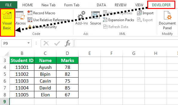
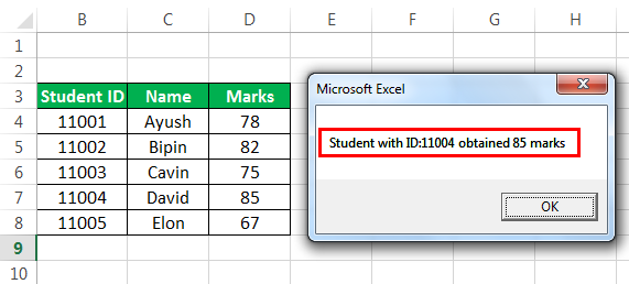
Suppose you have the data on students’ IDs, names, and average marks.
Now, you want to look up the marks obtained by a student with ID 11004.
To lookup for the value, follow the following steps:
- Go to the “Developer” tab and click on “Visual Basic.”
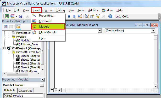
- Under the VBA window, go to “Insert” and click on “Module.”
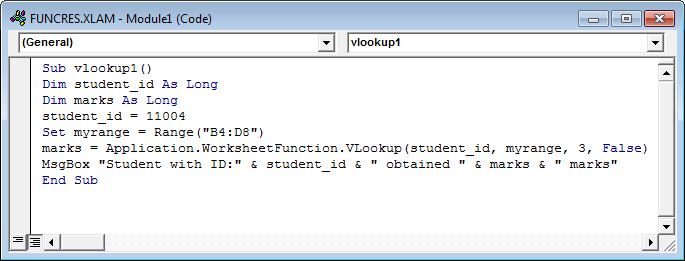
- Now, write the VBA VLOOKUP code. For example, we can use the following VBA VLOOKUP code.
Sub vlookup1()
Dim student_id As Long
Dim marks As Long
student_id = 11004
Set myrange = Range(“B4:D8”)
marks = Application.WorksheetFunction.VLookup(student_id, myrange, 3, False)
End Sub
Firstly, define a student ID, which is the lookup value. Therefore, we define:
student_id = 11004
Next, we define the range in which the value and the return value exist. Since our data is present in the cells B4:D8, we define a range- myrange as:
Set myrange = Range(“B4:D8”)
Finally, we input the VLOOKUP function using the Worksheet function in a variable marks as:
marks = Application.WorksheetFunction.VLookup(student_id, myrange, 3, False)
To print the marks in a message box, let us use the following command:
MsgBox “Student with ID:” & student_id & ” obtained ” & marks & ” marks”
It will return:
A student with ID:11004 obtained 85 marks.
Now, click the run button.
You will notice that a message box will appear in the Excel sheet.
VLookup Code in Excel VBA Example #2
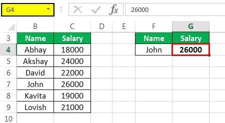
Suppose you have the data on the names of employees and their salaries. The data is in columns B and C. Next, you must write a VBA VLOOKUP code, given the employee’s name in cell F4. It will return the employee’s salary in cell G4.
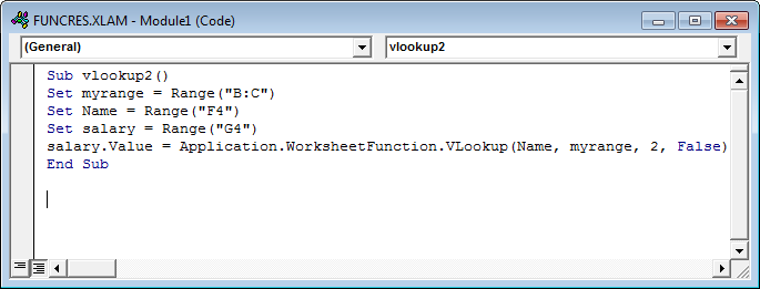
Let us write the VBA VLOOKUP code.
- Define the range in which the values are present, i.e., columns B and C.
Set myrange = Range (“B:C”)
- Define the employee’s name and input the name from cell F4.
Set name = Range (“F4”)
- Define salary as cell G4.
Set salary = Range (“G4”)
- Now, call the VLOOKUP function using WorksheetFunction in VBA and input it in salary.Value. It will return the value (output of the VLOOKUP function) in cell G4. We can use the following syntax:
salary.Value = Application.WorksheetFunction.VLookup(name, myrange, 2, False)
- Now, run the module. Cell G4 will contain the employee’s salary after you run the VBA VLOOKUP code.
Suppose you change the value of cell F4 to “David” in the worksheet and re-run the code, which will return David’s salary.
VLookup Code in Excel VBA Example #3
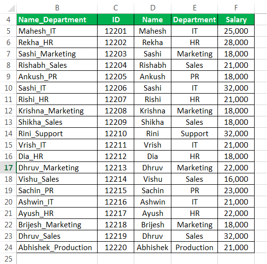
Suppose you have your company’s employees’ data, ID, names, Department, and salary. Using VLOOKUP in VBA, you want to get the salary details of an employee using his name and department.
Since the VLOOKUP function in Excel searches the lookup_value in only a single column, which is the first column of the table_array. It would help if you first made a column containing each employee’s “Name” and “Department.”
In VBA, let us insert the values “Name” and “Department” in column B of the worksheet.
To do this, go to the “Developer” tabEnabling the developer tab in excel can help the user perform various functions for VBA, Macros and Add-ins like importing and exporting XML, designing forms, etc. This tab is disabled by default on excel; thus, the user needs to enable it first from the options menu.read more and click “Visual Basic.” Then, go to “Insert” and click on “Module” to start a new module.
Let us now write code such that column B contains the values of column D (name) and column E.
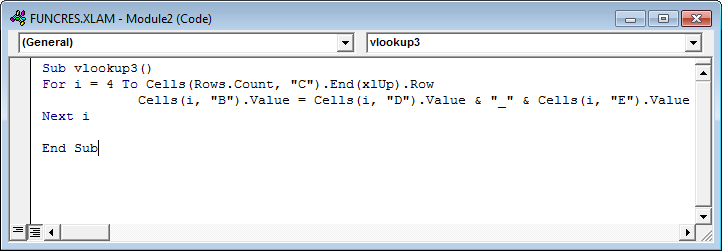
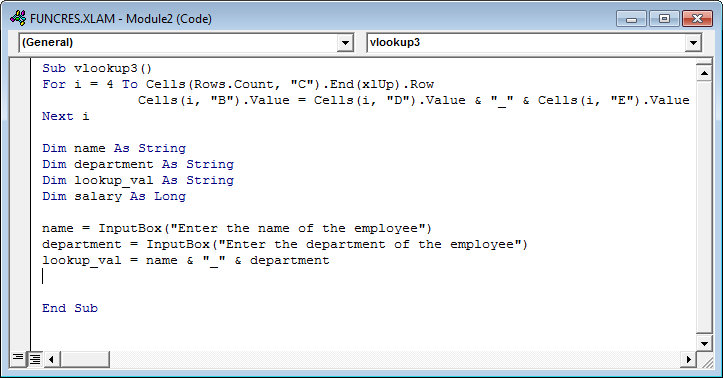
The syntax is:
Firstly, use a ‘for’ loop from i = 4 since the values start from the 4th row in this case. The loop will continue until the end of the last row of column C. So, we can use the variable as a row number inside the ‘for’ loop.
Then, enter the value to assign for Cell (row_number, column B), which we can give as Cells (i, “B”).Value, as Cell (row_number, column D) & “_” & Cell (row_number, column E).
Suppose you want to assign the cell B5 = D5 & “_” & E5. Then, you can simply use the code as:
Cells(5, “B”).Value = Cells(5, “D”).Value & “_” & Cells(5, “E”).Value
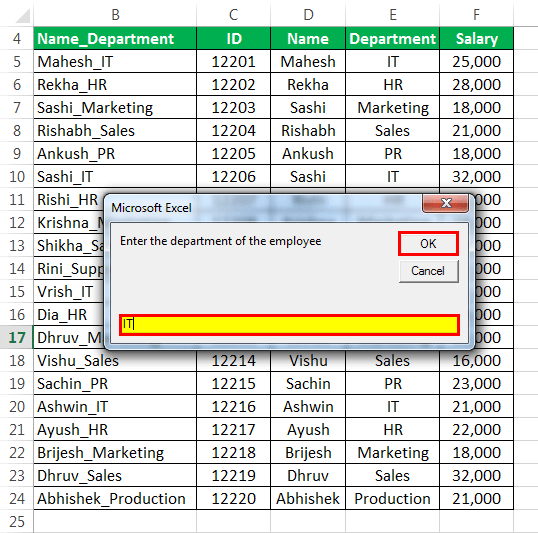
Now, let’s look for the lookup value in the array B5:E24. You need first to enter the lookup value. Let us take the value (Name and Department) from the user. To do this,
- Define three variables: name, department, and lookup_val as a string.
- Take the name input from the user. Use the code:
name = InputBox (“Enter the name of the employee”)
The content in the input box “Enter the ..” will be displayed in the prompt box when you run the code. The string entered in the prompt will be assigned to the name variable.
- Take the department from the user. We can do this similarly as above.
department = InputBox (“Enter the department of the employee”)
- Assign the name and department with “_” as a separator to the variable lookup_val using the following syntax:
lookup_val = name & “_” & department
- Write the VLOOKUP syntax to search for the lookup_val in range B5:E24 and return it in a variable salary.
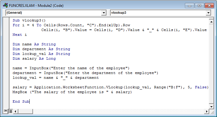
Initialize the variable salary:
Dim salary As Long
Use the VLOOKUP function to find the lookup_val. We can give the table_array as Range(“B:F”), and the salary is in the 5th column. We can thus use the following syntax:
salary = Application.WorksheetFunction.VLookup(lookup_val, Range (“B:F”), 5, False)
- To print the salary in a message box, use the syntax:
MsgBox (The salary of the employee is ” & salary)
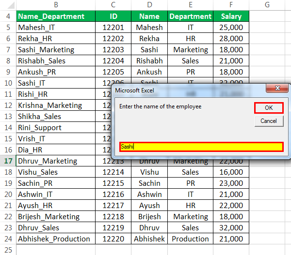
Now, run the code. A prompt box will appear in the worksheet where you can enter the name after you enter the name (Say “Sashi”) and click “OK.”
It will open another box in which you can enter the department. After you enter the department, say IT.
It will print the salary of the employee.
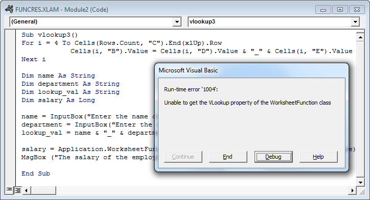
If VLOOKUP can’t find any employee with the name and department, it will give an error. For example, suppose you give the name “Vishnu” and the department “IT,” it will return “Run-time error ‘1004’.”
To address this issue, you can specify that on this type of error, print “Value not found” instead. To do this,
- Before using the vlookup syntax, use the following code:
On Error GoTo Message
Check:
The trailing code (of Check:) will be monitored, and if it receives an error, it will go to the “message” statement
- At the end of the code (Before End Sub), specify that if the error number is 1004VBA 1004 Error is a runtime error in VBA that is also known as an application-defined or object-defined error. Because Excel has a limited number of columns, we get a 1004 error when our code gives the command to go out of range.read more, then print in the message box, “Employee data not present.” One can do this using the syntax:
Message:
If Err.Number = 1004 Then
MsgBox (“Employee data not present”)
End If
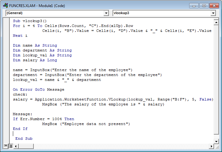
Module 1:
Sub vlookup3()
For i = 4 To Cells(Rows.Count, “C”).End(xlUp).Row
Cells(i, “B”).Value = Cells(i, “D”).Value & “_” & Cells(i, “E”).Value
Next iDim name As String
Dim department As String
Dim lookup_val As String
Dim salary As Longname = InputBox(“Enter the name of the employee”)
department = InputBox(“Enter the department of the employee”)
lookup_val = name & “_” & departmentOn Error GoTo Message
check:
salary = Application.WorksheetFunction.VLookup(lookup_val, Range (“B:F”), 5, False)
MsgBox (“The salary of the employee is ” & salary)Message:
If Err.Number = 1004 Then
MsgBox (“Employee data not present”)
End IfEnd Sub
Things to Remember About VLookup in Excel VBA
- The VLOOKUP function can be called in Excel VBA by using WorksheetFunction.
- The syntax of the VLOOKUP function remains the same in Excel VBA.
- When the VBA VLOOKUP code cannot find the lookup_value, it will give a “1004 error.”
- We can manage the error in the VLOOKUP function using a GoTo statement if it returns an error.
Recommended Articles
This article has been a guide to VLOOKUP in VBA. Here, we discuss writing VLOOKUP code in Excel VBA, practical examples, and a downloadable Excel template. You may learn more about Excel from the following articles: –
- Top Alternatives to Vlookup
- IFERROR with VLOOKUP in Excel
- VLOOKUP with Two Criteria
- Multiple Criteria of VLookup
VBA VLOOKUP Function (Table of Contents)
- Where to Write Macros?
- How to Use VBA VLOOKUP in Excel?
What is VBA VLOOKUP Function?
Vlookup function of excel can be used in the VBA as well with the same syntax that we used in Excel. Open a module in VBA and define a variable for Lookup value and then declare the cell where we will be applying Vlookup using VBA. Now as per syntax of Vlookup in VBA select the lookup value, lookup range or table, Column index number and range lookup is TRUE or FALSE. Now, if we run the code, then we will be able to see the lookup value in a declared cell in Excel.
Formula of VLOOKUP Function
The Formula includes 4 mandatory arguments.
- Lookup Value: This is the base values you are searching. Based on this we look for a value in the table.
- Table Value: This is the table which holds all the values. From this table using lookup value, we will fetch the data.
- Column Index Number: This is the column number from the table we are looking for. In a table, there are many columns, out of many columns we only require the column which we are looking for the data.
- Range Lookup: Here we need to specify what kind of result we want. If we want the exact match we need to mention as FALSE or 0, if we want the approximate match we can mention as TRUE or 1.
Where to Write Macros?
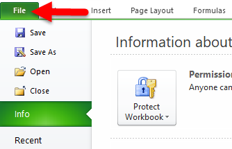
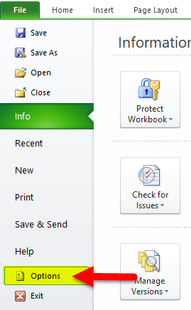
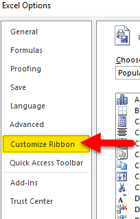
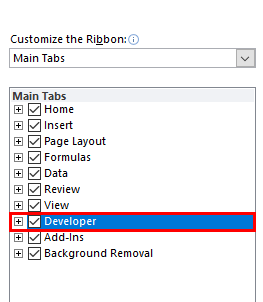
VBA is accommodated under Developer tab in excel. If you are not able to find the developer tab follow the below steps to unhide this.
Step 1: Click on File.
Step 2: Under File, click on Options.
Step 3: Select Customize Ribbon.
Step 4: On the right-hand side make sure the checkbox of the Developer tab is ticked.
Now you must see the Developer tab in the Ribbon.
How to Use VBA VLOOKUP Function in Excel?
VBA VLOOKUP Function is very simple to use. Let us now see how to use VBA VLOOKUP function in Excel with the help of some examples.
You can download this VBA VLOOKUP Excel Template here – VBA VLOOKUP Excel Template
Example #1
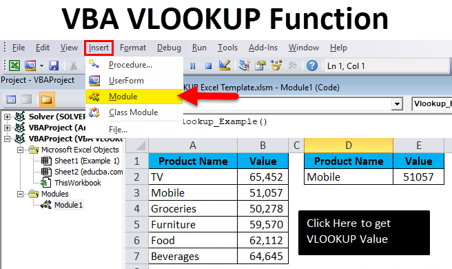
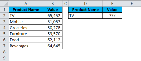
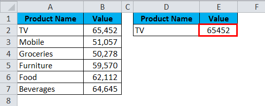
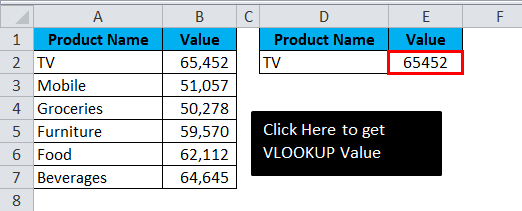
I have a sales table for different products. It has product name and sales made against that product.
In cell E2, I want to know the sales value of TV using VBA VLOOKUP function.
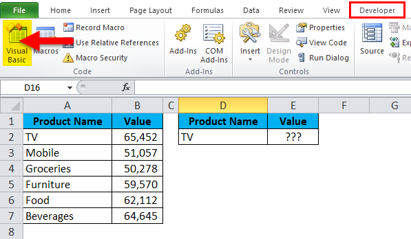
Step 1: Go to the Developer tab and click on Visual Basic
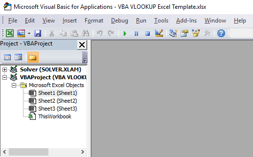
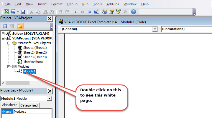
Step 2: Once you click on Visual Basic it will open the below window for you
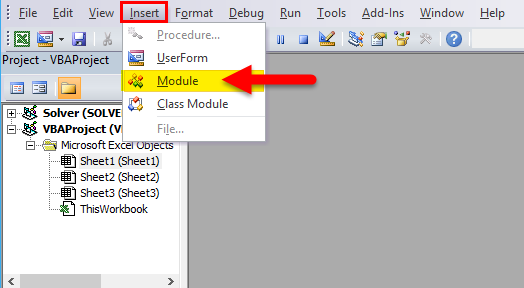
Step 3: Click on Insert and select Module
Step 4: Once you click on Module it will insert the new module for you. Double click on that newly inserted module to write your VLOOKUP code.
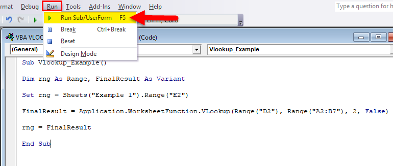
Step 5: Copy and paste the below code to your newly inserted module.
Sub Vlookup_Example()

Dim rng As Range, FinalResult As Variant

Set rng = Sheets("Example 1").Range("E2")

FinalResult = Application. WorksheetFunction. VLookup(Range("D2"), Range("A2:B7"), 2, False)

rng = FinalResult

End Sub
Let me break down the code to explain it to you.
Line 1: Dim rng as Range, FinalResult as Variant
This is the first line of the code. Using DIM statement I have declared two variables one is rng & another one is FinalResult.
Rng holds Range as the variable and FinalResult holds Variant as the variable.
Line 2: Set rng = Sheets(“Example 1”).Range(“E2”)
Previous declared variable rng is an object variable so we need to set to which range actually we are referring to. I have set the range to E2 cell. This is actually where I need the result to be displayed.
Line 3: FinalResult = Application. WorksheetFunction.VLookup (Range(“D2”), Range (“A2:B7”), 2, False)
This is the important line of the code. FinalResult holds the variable of the variant i.e. any kind of data type. FinalResugetsget the data from the function VLOOKUP.
Line 4: rng = FinalResult
Initial variable rng is equal to the value of FinalResult. Rng means E2 cell, FinalResult means value returned by the VLOOKUP function.
Step 6: Hit the RUN button or Press F5 to execute the code
Step 7: We will get the below output.
Example #2
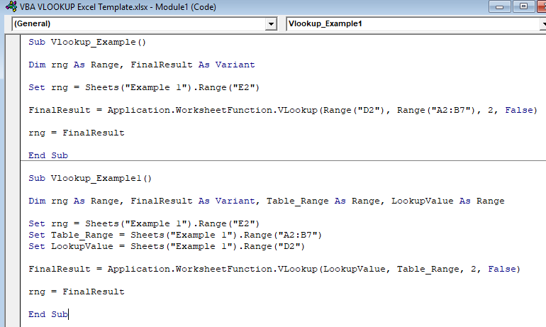
Take the same data from the above example. Here I am going to create names and apply the same in the VLOOKUP. The code will the same as the previous example. Only in VLOOKUP, I am changing references.
Sub Vlookup_Example1()

Dim rng As Range, FinalResult As Variant, Table_Range As Range, LookupValue As Range

Set rng = Sheets("Example 1").Range("E2")

Set Table_Range = Sheets("Example 1").Range("A2:B7")

Set LookupValue = Sheets("Example 1").Range("D2")

FinalResult = Application. WorksheetFunction. VLookup(LookupValue, Table_Range, 2, False)

rng = FinalResult

End Sub
Lookup value is set to D2 cell in the name of LookupValue. Table Array is set to A2 to B7 in the name of Table_Range.
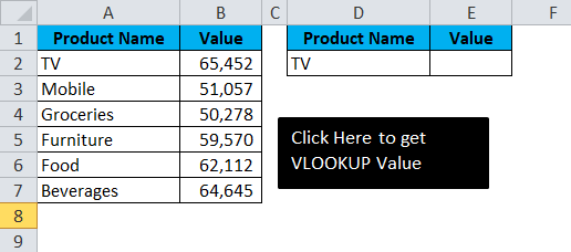
Create a Macro Button
Once the macro code is written we need to design the macro.
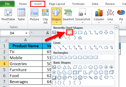
Step 1: Go to Insert and Select the rectangular shape.
Step 2: Draw a rectangular shape
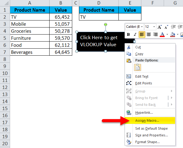
Step 3: Once the Rectangular shape has drawn right click on the rectangular shape and click on Assign Macro.
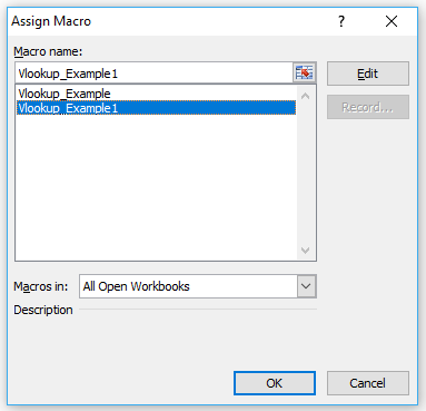
Step 4: Once you click on Assign Macro it will open up all the macro names. Select the macro name you wish to assign. I am assigning Example 1 macro name to the rectangular shape.
Step 5: Now rectangular shape has become a macro button. Once you click on the rectangular shape, you will get the below output.
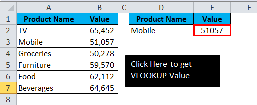
You can change the lookup value cell D2 and get the result. In the below image, I have changed the D2 cell value to Mobile.
Things to Remember About VBA VLOOKUP
- In VBA too VLOOKUP works the same as the worksheet function.
- Declaring variables and assigning data type is the important thing here.
- In the resulting cell, we do not see any kind of formula. Any value returned by VBA function does not hold any kind of formula.
Recommended Articles
This is a guide to Excel VBA VLOOKUP function. Here we discuss the VLOOKUP Formula and how to use VBA VLOOKUP in Excel along with practical examples and downloadable excel template. You can also go through our other suggested articles –
- VBA RGB
- VBA Create Object
- VBA Solver
- VBA Login
How to use VLOOKUP in Excel VBA: Step-by-Step (2023)
Visual Basic for Applications (VBA) has many built-in functions that help you work with spreadsheet data.
But “normal” Excel is the undisputed king when it comes to useful functions.
Fortunately, you can use worksheet functions to take advantage of that power when you’re writing macros in VBA.
First, you learn the differences between VBA functions and worksheet functions.
Then I show you how to use a worksheet function in VBA – the VLOOKUP!
Let’s dive in 🤿
Oh, and download the sample workbook here to tag along with this guide.
VBA functions vs. worksheet functions
VBA functions are built into Visual Basic for Applications, the scripting language that you use to create macros.
You can use VBA functions in any program that supports VBA (including Microsoft Word and Access).
Worksheet functions are specific to Excel. They’re the functions that you’re used to using in spreadsheets already—things like SUMIF, IF, and VLOOKUP.
You could get the same information from VBA without using worksheet functions—but in many cases, you’d have to write a lot of code that’s already been worked out in Excel.
Using worksheet functions saves you time overwriting your own functions in VBA.
To call a worksheet function, you’ll need to use the following syntax:
Application.WorksheetFunction.[function name]
Let’s walk through an example of a very useful function that isn’t present in VBA: the VLOOKUP function.
Using the VLOOKUP function in VBA
We’ll use a simple VLOOKUP formula example to see how worksheet functions can be called in VBA.
VLOOKUP is a very powerful function that’s great for finding information in big spreadsheets.
If you don’t remember, here’s what it does 🧠
VLOOKUP searches for a lookup value in a specified dataset. If it finds it, it returns a corresponding value from the same row.
Unfortunately, it’s not built into VBA. So we’ll have to call it with a worksheet function.
If you’re not familiar with the function, check out our full guide to VLOOKUP, which will walk you through it in detail.
Open the example workbook to follow along. It contains a list of product numbers and descriptions. We’ll use VBA code to look up descriptions based on product numbers.
Here’s the VBA code we’ll use:
Sub findProduct()
 Dim prodNum As Integer, prodDesc As String
 prodNum = Range("F2").Value
 prodDesc = Application.WorksheetFunction.VLookup(prodNum,
Range("A1:B51"), 2, FALSE)
 MsgBox prodDesc
End Sub
The first two lines of the script are simple; they declare prodNum as an integer variable and prodDesc as a String variable, then assign the value in cell F2 to prodNum.
F2 is the cell where we’ll ask users to input a product number.
The VBA VLOOKUP code is actually quite simple.
To use any Excel function in VBA, type “Application.WorksheetFunction.” and start typing the name of the function.
In this case, it’s “VLOOKUP”.
You’ll see it come up in the resulting list (you can also just type the name of the function you’re looking for).

Then you’ll need to include the standard arguments. In the VLOOKUP function, those are:
- lookup_number
- table_array
- col_index_num
- and range_lookup
You enter them similarly to how you would in Excel (if you’ve forgotten how to do that, read my guide here).
But there are a few differences ⚠️
In our case, lookup_number is the variable prodNum, which is similar to selecting a cell in Excel.
The table_array, however, needs to be presented in a format that VBA can handle. Here we’ve used Range(“A1:B51”), which selects the cells in A1:B51.
It’s important to remember that you can’t just type “A1:B51”, as VBA won’t recognize the range ⛔
col_index_num and range_lookup are the same as in Excel. We’re looking in the second column and want an exact match for the product number, so we’ll use 2 and FALSE.
So, use the below code to create a VBA VLOOKUP.
Application.WorksheetFunction.VLookup(prodNum, Range("A1:B51"), 2, FALSE)
Obviously, in those rare cases where you’ll actually need it, you can use approximate match in the 4th VBA VLOOKUP argument.
Make sure that there’s a product number (the lookup value) in F2:


VBA displays a message box with the matching product description for our product number.
This would be a great place to link a button to run a macro! Users would just have to enter the product number and click a button.
Why use worksheet functions in VBA?
This is more complicated than just using the function in Excel, so why would you write an Excel VBA macro for a VLOOKUP function?
Any function that’s present in Excel is going to be slightly more complicated to use in VBA code. But having access to them gives you the option of very powerful automation.
For example, if you wanted to run multiple VLOOKUPs and have the results put in a table, you might find that you need to manually create each VLOOKUP in Excel ⚙️
Or you could write Excel VBA code with the VBA VLOOKUP function that automates the process and saves you time. Even if it is possible to use functions in Excel, it will likely be much more efficient in VBA. You can also save the script and run it on other spreadsheets.
Remember that you can use almost any Excel function from within VBA. Just type “Application.WorksheetFunction.” and you’ll see options in the VBA window.
You can also call these functions with Application.[function name].
But when you’re getting started, use the full line with “WorksheetFunction.”
That’s it – Now what?
Well done learning VLOOKUP in VBA. It wasn’t so hard, was it? 🤞
Once you’ve learned to use Excel’s worksheet functions from within Excel VBA, you’re ready to start writing some very powerful VBA code.
Although it’s useful, the VBA VLOOKUP code is just a tiny part of VBA.
If you want to dive deeper into Excel VBA and see some practical examples, enroll in my free 30-minute VBA training course here.
Other resources
If you’re a little rusty on the arguments of the VLOOKUP function: exact or approximate match, the lookup value, the column index number, or the table array – you might want to read up on it here.
Frequently asked questions
Yes, you can use the VBA VLOOKUP code here:
Application.WorksheetFunction.VLookup(prodNum, Range(“A1:B51”), 2, FALSE)
Beware you can actually use the VLOOKUP in VBA. Its syntax is used a tiny bit differently than when you use the worksheet version – but it’s not much.
If you really don’t want to use VBA VLOOKUP, you can use VBA INDEX MATCH instead.
Kasper Langmann2023-01-30T20:01:22+00:00
Page load link


