
Excel for Microsoft 365 Excel for Microsoft 365 for Mac Excel for the web Excel 2021 Excel 2021 for Mac Excel 2019 Excel 2019 for Mac Excel 2016 Excel 2016 for Mac Excel 2013 Excel 2010 Excel 2007 Excel for Mac 2011 Excel for Windows Phone 10 More…Less
This topic describes the most common VLOOKUP reasons for an erroneous result on the function, and provides suggestions for using INDEX and MATCH instead.
Tip: Also, refer to the Quick Reference Card: VLOOKUP troubleshooting tips which presents the common reasons for #NA issues in a convenient PDF file. You can share the PDF with others or print for your own reference.
Problem: The lookup value is not in the first column in the table_array argument
One constraint of VLOOKUP is that it can only look for values on the left-most column in the table array. If your lookup value is not in the first column of the array, you will see the #N/A error.
In the following table, we want to retrieve the number of units sold for Kale.

The #N/A error results because the lookup value “Kale” appears in the second column (Produce) of the table_array argument A2:C10. In this case, Excel is looking for it in column A, not column B.
Solution: You can try to fix this by adjusting your VLOOKUP to reference the correct column. If that’s not possible, then try moving your columns. That may also be highly impracticable, if you have large or complex spreadsheets where cell values are results of other calculations—or maybe there are other logical reasons why you simply cannot move the columns around. The solution is to use a combination of INDEX and MATCH functions, which can look up a value in a column regardless of its location position in the lookup table. See the next section.
Consider using INDEX/MATCH instead
INDEX and MATCH are good options for many cases in which VLOOKUP does not meet your needs. The key advantage of INDEX/MATCH is that you can look up a value in a column in any location in the lookup table. INDEX returns a value from a specified table/range—according to its position. MATCH returns the relative position of a value in a table/range. Use INDEX and MATCH together in a formula to look up a value in a table/array by specifying the relative position of the value in the table/array.
There are several benefits of using INDEX/MATCH instead of VLOOKUP:
-
With INDEX and MATCH, the return value need not be in the same column as the lookup column. This is different from VLOOKUP, in which the return value has to be in the specified range. How does this matter? With VLOOKUP, you have to know the column number that contains the return value. While this may not seem challenging, it can be cumbersome when you have a large table and have to count the number of columns. Also, if you add/remove a column in your table, you have to recount and update the col_index_num argument. With INDEX and MATCH, no counting is required as the lookup column is different from the column that has the return value.
-
With INDEX and MATCH, you can specify either a row or a column in an array—or specify both. This means you can look up values both vertically and horizontally.
-
INDEX and MATCH can be used to look up values in any column. Unlike VLOOKUP—in which you can only look up to a value in the first column in a table—INDEX and MATCH will work if your lookup value is in the first column, the last, or anywhere in between.
-
INDEX and MATCH offer the flexibility of making dynamic reference to the column which contains the return value. This means that you can add columns to your table without breaking INDEX and MATCH. On the other hand, VLOOKUP breaks if you need to add a column to the table—since it makes a static reference to the table.
-
INDEX and MATCH offers more flexibility with matches. INDEX and MATCH can find an exact match, or a value that is greater or lesser than the lookup value. VLOOKUP will only look for a closest match to a value (by default) or an exact value. VLOOKUP also assumes by default that the first column in the table array is sorted alphabetically, and suppose your table is not set up that way, VLOOKUP will return the first closest match in the table, which may not be the data you are looking for.
Syntax
To build syntax for INDEX/MATCH, you need to use the array/reference argument from the INDEX function and nest the MATCH syntax inside of it. This take the form:
=INDEX(array or reference, MATCH(lookup_value,lookup_array,[match_type])
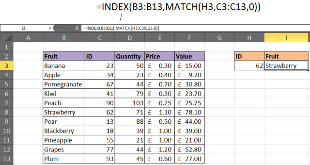
Let’s use INDEX/MATCH to replace VLOOKUP from the example above. The syntax will look like this:
=INDEX(C2:C10,MATCH(B13,B2:B10,0))
In simple English it means:
=INDEX(return a value from C2:C10, that will MATCH(Kale, which is somewhere in the B2:B10 array, in which the return value is the first value corresponding to Kale))
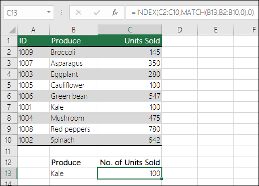
The formula looks for the first value in C2:C10 that corresponds to Kale (in B7) and returns the value in C7 (100), which is the first value that matches Kale.
Problem: The exact match is not found
When the range_lookup argument is FALSE—and VLOOKUP is unable to find an exact match in your data—it returns the #N/A error.
Solution: If you are sure the relevant data exists in your spreadsheet and VLOOKUP is not catching it, take time to verify that the referenced cells don’t have hidden spaces or non-printing characters. Also, ensure that the cells follow the correct data type. For example, cells with numbers should be formatted as Number, and not Text.
Also, consider using either the CLEAN or TRIM function to clean up data in cells.
Problem: The lookup value is smaller than the smallest value in the array
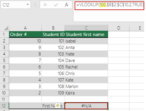
If the range_lookup argument is set to TRUE—and the lookup value is smaller than the smallest value in the array—you will see the #N/A error. TRUE looks for an approximate match in the array and returns the closest value lesser than the lookup value.
In the following example, the lookup value is 100, but there are no values in the B2:C10 range that are lesser than 100; hence the error.
Solution:
-
Correct the lookup value as necessary.
-
If you cannot change the lookup value and need greater flexibility with matching values, consider using INDEX/MATCH instead of VLOOKUP—see the section above in this article. With INDEX/MATCH, you can look up values greater than, lesser to, or equal to the lookup value. For more information on using INDEX/MATCH instead of VLOOKUP, refer to the previous section in this topic.
Problem: The lookup column is not sorted in the ascending order
If the range_lookup argument is set to TRUE—and one of your lookup columns is not sorted in the ascending (A-Z) order—you will see the #N/A error.
Solution:
-
Change the VLOOKUP function to look for an exact match. To do that, set the range_lookup argument to FALSE. No sorting is necessary for FALSE.
-
Use the INDEX/MATCH function to look up a value in an unsorted table.
Problem: The value is a large floating point number
If you have time values or large decimal numbers in cells, Excel returns the #N/A error because of floating point precision. Floating point numbers are numbers that follow after a decimal point. (Excel stores time values as floating point numbers.) Excel cannot store numbers with very large floating points, so for the function to work correctly, the floating point numbers will need to be rounded to 5 decimal places.
Solution: Shorten the numbers by rounding them up to five decimal places with the ROUND function.
Need more help?
You can always ask an expert in the Excel Tech Community or get support in the Answers community.
See Also
-
Correct a #N/A error
-
VLOOKUP: No more #NA
-
Floating-point arithmetic may give inaccurate results in Excel
-
Quick Reference Card: VLOOKUP refresher
-
VLOOKUP function
-
Overview of formulas in Excel
-
How to avoid broken formulas
-
Detect errors in formulas
-
All Excel functions (alphabetical)
-
All Excel functions (by category)
Need more help?
When VLOOKUP can’t find a value in a lookup table, it returns the #N/A error. In this example, the goal is to remove the #N/A error that VLOOKUP returns when it can’t find a lookup value. In general, the best way to do this is to use the IFNA function. However, the IFERROR function can also be used in the same way. Both options are explained below.
VLOOKUP function
The VLOOKUP function performs a lookup operation on vertical data. The generic syntax for VLOOKUP looks like this:
VLOOKUP(A1,table,column,FALSE)Where A1 contains a value to lookup, table is the data, column is a number, and FALSE specifies exact match, which is required in this example. In the workbook shown, we want to enter an abbreviation in cell E5 and get the correct State name in cell F5, where all data is in an Excel Table named data. To do this, we can use VLOOKUP in a formula like this:
VLOOKUP(E5,data,2,FALSE)When a valid 2-letter code is entered in cell E5, VLOOKUP will return the corresponding State. For example, if «CA» is entered in cell E5, VLOOKUP will return «California»:
VLOOKUP("CA",data,2,FALSE) // returns "California"If an invalid code is entered in cell E5, VLOOKUP will return an #N/A error:
VLOOKUP("XX",data,2,FALSE) // returns #N/AThe screen below shows how this error looks on the worksheet:

The #N/A error technically means «not available». However, you may want to return a more friendly result. You can do this by combining VLOOKUP with the IFNA function.
VLOOKUP with IFNA
The IFNA function is a simple way to trap and handle #N/A errors without catching other errors. When used with a formula, the generic syntax for NA looks like this:
=IFNA(formula,alternative)where formula might return a #N/A error and alternative is the value or formula to return in that case. To trap the #N/A error in this example, we wrap the IFNA function around the original VLOOKUP function and provide an alternate value. For example, to return «Not found» when VLOOKUP returns #N/A, we can use a formula like this:
=IFNA(VLOOKUP(E5,data,2,FALSE),"Not found")Now when VLOOKUP returns the #N/A error, IFNA takes over and returns «Not found»:
=IFNA(VLOOKUP("XX",data,2,FALSE),"Not found") // returns "Not found"To return a different message, just change the second argument in IFNA:
=IFNA(VLOOKUP("XX",data,2,FALSE),"Invalid code") // returns "Invalid code"If you would prefer to return nothing, you can provide an empty string («») instead like this:
=IFNA(VLOOKUP("XX",data,2,FALSE),"") // returns ""The result from this formula will look like an empty cell when the lookup Code is not found.
VLOOKUP with IFERROR
You can also trap #N/A errors returned by VLOOKUP with the IFERROR function like this:
=IFERROR(VLOOKUP(E5,data,2,FALSE),"Not found")IFERROR works just like the IFNA function — it catches an #N/A error returned by VLOOKUP and returns an alternative result. The difference is that IFERROR will catch other errors as well.
Note: The #N/A error is Excel’s way of telling you a value was not found. With the more general IFERROR function, there is a risk that you might catch another unrelated errors and return a confusing result. For example, if you have a typo in your formula, Excel might return the #NAME! error. Or, if rows/column are deleted in a worksheet, a formula might return a #REF! error. While IFNA will let these errors come through, alerting a user to a different problem, IFERROR will catch these errors too and the alternative result may obscure problems. For these reasons, I prefer to use IFNA when the purpose is to trap #N/A errors only.
Older versions of Excel
In earlier versions of Excel that lack the IFNA function, you will need to repeat the VLOOKUP inside an IF function that catches an error with the ISNA function. For example:
=IF(ISNA(VLOOKUP(A1,table,2,FALSE)),"Not found",VLOOKUP(A1,table,2,FALSE))
Overview:
Fed up of this Excel VLookup not working issue? Do you have any idea why is VLOOKUP not working OR how to fix this?
If not….THEN go through this article as it cover all the reasons of Excel VLOOKUP not working and their fixes.
To recover lost Excel data, we recommend this tool:
This software will prevent Excel workbook data such as BI data, financial reports & other analytical information from corruption and data loss. With this software you can rebuild corrupt Excel files and restore every single visual representation & dataset to its original, intact state in 3 easy steps:
- Download Excel File Repair Tool rated Excellent by Softpedia, Softonic & CNET.
- Select the corrupt Excel file (XLS, XLSX) & click Repair to initiate the repair process.
- Preview the repaired files and click Save File to save the files at desired location.
In this section, you will get an answer to this very important question why is VLookup not working. So, check out the 7 most common reasons for VLOOKUP not working in Excel 2007/2010/2013/2016/2019.
Have a look…
- VLOOKUP Can’t Find Value
- Table Reference Is Locked
- Column Insertion
- Oversized Table
- VLOOKUP Cannot Look To Its Left
- Not Getting The Exact Match
- Excel Table Has Duplicate Values
Reason 1# VLOOKUP Can’t Find Value
Excel user who all are using VLOOKUP, MATCH, or HLOOKUP functions every now and then encountered some unexpected #N/A error.
Usually, this error encounters when anyone tries to match the Excel lookup value within the array. It’s a clear sign that your Excel function has been failed to fetch lookup value from the lookup array.
What will you do if you will see that the exact matching value is there in the lookup array but your excel application is unable to find that value?
Suppose: if in the shown Excel spreadsheet, lookup function is applied. You want to look up the value “1110004” of the cell to get a match with the value “1110004” present in cell E6.

In this case, if the Excel function fails to fetch the match or showing error #N/A error. The VLOOKUP function is a popular lookup and reference function of Excel. It will show a tricky and dreaded #N/A error message. It may happen because Excel is not considering the two values exactly the same.
Reason 2# Table Reference Is Locked
If you are using multiple VLOOKUPs in excel to catch different information about any particular record. or if in case you are willing to copy off your VLOOKUP to several of your cells then you have to check your table.
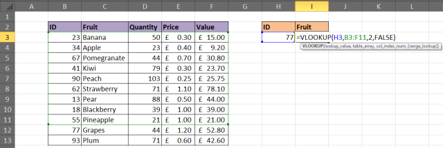
The below-shown image shows that the VLOOKUP entered over here is incorrect. The incorrect cell ranges are referenced for the lookup_value and table array.

Solution
The table which is used by VLOOKUP function actually searches for and gives information is called astable_array. This is required to get referenced completely in order to copy your VLOOKUP.
So, click on the references which are right inside the formula and after then press the F4 key on your keyboard to modify the reference from relative to absolute. So, enter the formula as=VLOOKUP($H$3,$B$3:$F$11,4,FALSE).
In this example, both the lookup_value and table_array references made were absolute. Basically, it may be the table_array that needs locking.
Reason 3# Column Insertion
The column index number or col_index_num is used by the VLOOKUP function in order to enter information to return a record.
Because this is entered as an index number, and it is not that durable. If a column is put down in the table, then vlookup is not working as this stops VLOOKUP from working. Here is the image is shown below for a scenario.

The whole content is in column 3, but after the insertion of the new column, it became column 4. However, the VLOOKUP has not automatically updated.
Solution 1
One solution you can try to save your worksheet so any other user can’t insert columns. If the user requires to do so, then it’s not a valid solution.
Solution 2
Another option is to insert the MATCH function within the col_index_num argument of VLOOKUP.
The MATCH function can be used to search for something or returning the required column number. This will; makes the col_index_num dynamic so that the inserted columns won’t affect the VLOOKUP.
The formula given below needs to be entered within this example to avoid the above-mentioned problem.
Reason 4# Oversized Table
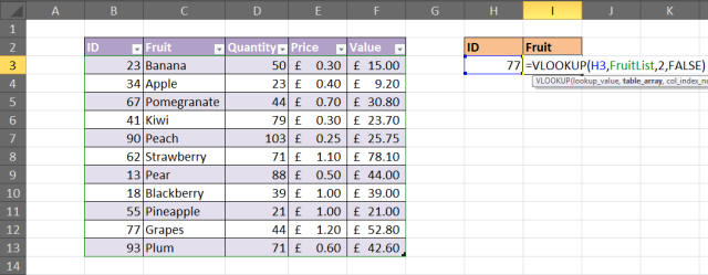
When more rows get added to the table, VLookup requires to get updated. Below given image shows that VLookup doesn’t check complete table fruit items.
Solution
You can consider the formatting range as a dynamic range name or table (Excel 2007+). This process ensures that VLookup will look over the complete of your table.
In order to format the range as a table, choose the cell range that you want to use for table_array. After then tap to the Home > Format as Table and choose any one style from the gallery section. Tap to the Design tab present within Table Tools and then change the table name in the given box.
The VLOOKUP below shows a table named FruitList being used.
Reason 5# VLOOKUP Can’t Look On It’s Left
The limitation of the VLOOKUP function is that it can’t look at its left. This will appear at the left-most column of a table and return information from the right.
Solution
The solution to fix the VLOOKUP not working issue is not to use VLOOKUP at all. You can use the combination of INDEX and MATCH Excel function as an alternative for VLOOKUP.
The below given example is to show what information is returned to the left of the column you are looking in.
Reason 6# Not Getting The Exact Match
In the ending argument of VLOOKUP function, well known as range_lookup, you can search for the approximate or an exact match.
In most cases, users look for particular product order, employee or customer and therefore require and an exact match. if you are searching for any unique value, enter FALSE for the range_lookup argument.
This one is optional, but if it is left unfilled then the TRUE value must be used. The TRUE value relies on your data is sorted in order to work.
The Below shown figure will show a VLOOKUP with the range_lookup argument omitted and the incorrect value being returned.

Solution
If looking for some unique value then enter FALSE value for the ending argument. The VLOOKUP must be entered like =VLOOKUP(H3,B3: F11,2,FALSE).
This is the first reason behind the VLookup not working in Excel.
Reason 7# Excel Table Has Duplicate Values
Excel VLOOKUP function is limited to return only one record. It gives 1st record which matches the value you are searching for.
If your Excel table is having some duplicates then VLOOKUP fails to perform this task.
Solution
In the shown list some duplicates values are present. In this case, VLOOKUP is not the right choice to use. PivotTable is the perfect option to choose the value and then listing out the result.
Below shown table is to shows a list of orders. Suppose you are willing to return the entire order of any specific fruit.

PivotTable allows you to choose the Fruit ID from the report filter and the list of all orders starts appearing.

These are the 7 Best reasons behind VLOOKUP not working error in Excel. Hopefully, now the Excel VLOOKUP won’t work issue is fixed but if not then make use of the automatic solution to fix VLOOKUP won’t working error in Excel.
FAQ:
Why Can’t VLOOKUP Find Value?
VLOOKUP fails to find Value when the lookup value doesn’t exist in the source data.
When VLOOKUP can’t find the value it starts showing #N/A error. This same error also encounters when HLOOKUP, LOOKUP, or MATCH functions fail to find values.
How Do I Enable VLOOKUP In Excel?
Here are the steps to enable VLOOKUP In Excel.
1. Go to the formula tab, and then from the Function Library group make a tap over the Insert Function icon.
2. Now from the opened dialog box of Insert Function:
- Either in the search box type “VLOOKUP” or from the select a category section you can choose Lookup & Reference option.
- Now from the section of Select a function, choose VLOOKUP.
- Tap the OK button.

3. Within the dialog box of Function Arguments.
- Assign following data Lookup_value ,Table_array, Col_index_num, Range_lookup.
- If you don’t feel up these data then Excel will count it as True.
4. Hit the OK button.
Automatic Solution: MS Excel Repair Tool
The given manual solution will surely fix off your Excel file issues and errors. but if in case you are caught in any other corruption glitches or damaged file issues then make use of MS Excel Repair Tool. It is the best-suited software for restoring down the corrupt Excel files and also for the retrieval of data from Excel worksheets like cell comments, charts, worksheet properties, and other stuff. It’s a professionally designed program that easily repairs .xls and .xlsx files.
* Free version of the product only previews recoverable data.
Steps to Utilize MS Excel Repair Tool:
Conclusion
Troubleshooting problems regarding Excel worksheets formula and functions can be a big job. Actually, the error comes with the package. Though Excel offers some auditing tools, which are present under the Formula Auditing group of Formulas tab, so you don’t always need to apply much effort in fixing up these relative issues.
Sometimes just a bit of Excel special knowledge can help you to resolve issues that occurred with such Excel formulas and functions.
I tried my best to provide ample information about the VLOOKUP is not working error in Excel. However, if you are having any additional fixes or any query then please share them with us. You can go to the comment section.
Good Luck…


Priyanka is an entrepreneur & content marketing expert. She writes tech blogs and has expertise in MS Office, Excel, and other tech subjects. Her distinctive art of presenting tech information in the easy-to-understand language is very impressive. When not writing, she loves unplanned travels.
VLOOKUP error in Excel
Ever have this happen? You write your VLOOKUP formula and have one of the following values returned:
- #VALUE!
- #NAME?
- #N/A
- #REF!
- Other UNEXPECTED result!
Below you’ll find some common pitfalls that cause each of the errors above.
VLOOKUP function syntax
First, here’s a recap of the usage syntax for the VLOOKUP function in Excel. I’ll be referring to the parts in the explanations below.
VLOOKUP(lookup_value, table_array, column_index_number, [range_lookup])
For more detail on the arguments, see the function’s documentation page.
VLOOKUP errors in Excel
#VALUE! error causes in VLOOKUP
column_index_number is less than 1
In an effort to retrieve a value that is to the left of the lookup column, you may be tempted to put in a value less than one. However, VLOOKUP only finds values starting with the lookup column, and counting over to the right.
If you need to look up values that actually sit to the left of the lookup column, you can. Just use a combination of the INDEX and MATCH functions. To see how this is done, read “Do you need your VLOOKUP to look to the left instead of the right?“
Your table_array reference isn’t correct
If you’re using a named range, did you use the correct name? It’s worth double-checking to make sure you selected the correct range name.
Or, if you entered a range was it an absolute range or relative?
If you used A2:C5, and your VLOOKUP is filled down in a table, you will have A3:C6, A4:C7, etc. which is likely not what you expect or need. Instead, use the absolute reference form of $A$2:$C$5.
The lookup_value is longer than 255 characters
This is a limit within Excel.
An option is to use the INDEX and MATCH functions instead.
#NAME? error causes in VLOOKUP
This happens when you type the name of the function incorrectly. Basically, just make sure you spelled “VLOOKUP” correctly. That’s all.
#N/A error causes in VLOOKUP
The lookup_value does not exist in the lookup column
Did you have a typo? Double-check to be sure the value you’re searching is typed correctly.
It’s also possible that the value simply is not in the list. If you’d rather return something friendly than “#N/A” to your worksheet, use the ISNA function. I prefer simply to use IFERROR, but it catches all the errors and not just #N/A. You may have something like the following.
=IFERROR(VLOOKUP(lookup_value, table_array, column_index_value, [range_lookup]), "Value not found")
Leading or trailing spaces in your lookup_value data
If you think you may have leading or trailing spaces in your lookup_value data, you can use the TRIM function in Excel to remove them before and after your data. You may change your function call to something like the following.
=VLOOKUP(TRIM(lookup_value), table_array, lookup_column_value, [range_lookup])
The format of the lookup_value is not the same as the data
Does your data have the same number format as your lookup_value data? Are your numbers formatted as text. Data from a data source may be loaded into Excel as text — even though it looks like a number. If you think your lookup_values may be formatted as text, you can either change the number formatting of the column. Choose Number in the drop down list in the Number group in the ribbon.
You can also use the NUMBERVALUE function. It will convert text (even if it has commas in it) numbers into the numerical values. You may have the following in your VLOOKUP function.
=VLOOKUP(NUMBERVALUE(lookup_value), table_array, lookup_column_value, [range_lookup])
Special characters in the lookup_value or data
Carriage returns, etc can cause VLOOKUP problems. Be sure your data doesn’t contain special characters.
You’re not using the first column as the lookup column
The first column is always the lookup column. You cannot use a column to the left by providing a negative number for the column_index_number.
If you need to retrieve data to the left of your lookup column, you can. Just use a combination of the INDEX and MATCH functions. To see how this is done, read Do you need your VLOOKUP to look to the left instead of the right?
range_lookup not working as expected
Incorrect use of the range_lookup feature
The help text for range_lookup says to use TRUE for an “approximate match”. However, this has nothing to do with any sort of fuzzy matching of a text lookup. If you want to perform a fuzzy match for the VLOOKUP, see Fuzzy VLOOKUP in Excel for information.
Lookup data unsorted
If you are looking for a value nearest your lookup value, is your lookup column sorted in ascending order? This is required when range_lookup is TRUE.
lookup_value too small
If your lookup_value is less than the smallest value in the lookup column, the range_lookup will also fail when set to TRUE.
#REF! error causes in VLOOKUP
When you see this error returned, make sure the column_index_number is not greater than the number of columns in your table_array range.
Unexpected (non-error) value
Unexpected value returned? Here are some common causes.
You expected a case sensitive lookup
VLOOKUP does a case insensitive comparison. So, MYVALUE, MyValue, Myvalue, myvalue are all the same as far as VLOOKUP is concerned.
VLOOKUP only returns the first value found
VLOOKUP starts at the top and looks for your value. It will stop at the first value found.
Want to know why your Excel VLOOKUP is not working? You are in the right place. This tutorial will help you learn why you are getting VLOOKUP errors in Excel 2019, 2016, 2013, 2010 and 2007.
Introduction to Excel VLOOKUP Not Working
Most of the Excel gods consider VLOOKUP as their favorite Excel function. If you manage to master this function, then you are qualified to brag a little about your Excel knowhow since you can solve many problems with it.
You can do so much cool stuff if you get to understand the nuts and bolts about the VLOOKUP function, how it works, why it fails to work sometimes, and how to fix any “Excel VLOOKUP not working” problem.
We all know how powerful the VLOOKUP function is, yet it isn’t flawless. Just like most useful things, it too has its side effects. In this topic, I want to talk about some of the things that trip up the VLOOKUP function.
But first, if you are not familiar with this function, you should get to know what it means in plain English. Just click here to read a blow-by-blow guide to the VLOOKUP function.
Now, using the following VLOOKUP cases, let’s see how to deal with the most common VLOOKUP error message: #N/A Error.
What is #N/A Error in VLOOKUP?
In Excel, #N/A means The Value isn’t Available. This error is very common in performing lookup or statistical functions.
Let’s take the VLOOKUP function, for example, if you use it to look up a range and it can’t find what it is supposed to look for, it will give you the #N/A error message.
Therefore, VLOOKUP #N/A error is Excel’s way of telling you that the lookup value is not found in the first column of the lookup table.
Consider the following VLOOKUP example.
At the right-hand side is a table containing employee information including employee name, occupation, hire date and salary details. At the left-hand side is also a small table that uses the VLOOKUP function to fetch the annual salary based on the name selected.
See screenshot:

Causes of Excel VLOOKUP Not Working and Solutions
Now let’s look at the circumstances under which the VLOOKUP function will generate an error and how to address these errors.
#1. You mistyped the lookup value
The lookup value is what the function is supposed to search for in the lookup table.
If for any reason you mistyped the lookup value, the function will not find what you typed and will definitely give you an error message.
For instance, instead of typing Daniel Chloe you mistyped Daniel Kloe as the lookup value. For you, these two names may sound the same but Excel sees them as different names.
See screenshot:

As seen in the above screenshot, the VLOOKUP function displayed the #N/A error message when the employee name was mistyped. But when the name was typed correctly, the formula was now able to find the specified employee’s salary.
The solution to this kind of Excel VLOOKUP not working problem is simply to retype the mistyped value correctly.
#2. Leading and trailing spaces
Like in the above case, the problem disappeared as soon as the user fixe the problem by typing the employee name correctly. Sometimes it is not that easy.
See the example below:

Look at the above example. The data, as well as the VLOOKUP formula, is the same as the previous example. Everything looks correct now. This time around the name is spelled correctly. But why do you have this error message? Why can you see this but Excel cannot?
Well, this kind of error takes more than just the eyes to see. This is caused by extra spaces which your eyes can hardly see, especially when dealing with a large volume of data.
Solution:
The solution to this kind of Excel VLOOKUP not working problem is to check and see where there are extra spaces and get rid of them. Extra spaces in the main table (lookup column) can cause the error just like extra spaces in the lookup value.

Another way to solve this problem is to use the TRIM function within the VLOOKUP formula.
The trim function removes extra spaces from your cells. Thus, if the extra spaces are in the lookup value (cell B6), instead of looking up B6, look up TRIM(B6).
With this trick, even if there happen to be leading and trailing spaces in your lookup value, the trim function will always handle that for you.

However, the extra spaces could be in your lookup table as well. If that’s the case, you’ll make sure you get rid of that too or the error won’t leave you alone.
See screenshot:

#3. Numbers formatted as text
This is another thing to look at when your Excel VLOOKUP formula is not working.
When your function is supposed to search for numbers, but instead it searches for text (or vice versa), Excel will give you an error message.
This kind of errors normally occurs when the data is imported from an external database or maybe you’ve typed an apostrophe before a number.
Numbers can be formatted as text though, but Excel will still alert you with a warning message (sign) that say’s “hey buddy, these are numbers but they are stored as text”.
See screenshot:

Solution:
To solve this problem, all you have to do is format the cell or cells using the number format. If it is just one cell, simply click the warning sign, and select Convert to Number.

But for multiple cells, select them all, and go to the Home tab, in the Number category there’s a drop-down arrow, click it and select the Number format.
#4. You are using an Approximate Match
In VLOOKKUP, the fourth argument is always optional and you can decide to give it no argument.
You should beware though, as Excel will assign an argument for you by default which in most cases leads to Excel VLOOKUP not working.
Unless you know what you are up to, you should always use FALSE (which means Exact Match) as your fourth VLOOKUP argument.
If you don’t use an Exact Match (i.e. FALSE), then you are heading for trouble.
Why is that?
If you don’t specify the fourth argument (using FALSE for Exact Match), Excel will assume you want an approximate match (using TRUE as a fourth argument).
The approximate match is rarely used when writing real-world VLOOKUP functions. VLOOKUP with an approximate match works completely different from Exact Match which is why you should always stick to using the Exact match.
However, there are some few exceptions. You can use 0 (the number zero) which technically is the same as FALSE. But never leave this argument when writing your VLOOKUP formula because Excel will assign it for you with an approximate match (i.e. True).
Another exception is those who use the VLOOKUP function as a replacement to nested IF statements to solve more sophisticated solutions. Accountants are living examples of those who use VLOOKUP with an approximate match, but that too only 0.99% of the time.
Therefore, if you are not a very clever Excel Rockstar, and you are not also creating a complex system which requires the use of Approximate match, always write your VLOOKUP formula with the Exact match.
#5. Using an Exact Match
As I mentioned previously, it is always a good practice to write your VLOOKUP function using an exact match as your last argument. But it also means that when Excel doesn’t find the value you are looking for in the lookup table, you will definitely get an error.
The reasons why Excel may not find your search has already been addressed above, which includes mistyping of lookup values, leading and trailing spaces and sometimes when numbers are formatted as text and vice versa.
Now let’s look at the some other VLOOKUP errors that may occur when writing formulas.
#NAME? error in VLOOKUP
This error is normally caused by a typo. It simply means that Excel can’t find the name of the function you used.

Below are some of the circumstances that may lead to #NAME? error in VLOOKKUP.
- When VLOOKUP contains text not enclosed in quotation marks.
- When VLOOKUP function name is misspelled.
- When VLOOKUP formula contains an undefined range or cell name.
- When the VLOOKUP formula omits the colon between the cell addresses of a range reference (lookup table)
When you encounter the #NAME? error in your VLOOKUP formula, you can quickly find a solution by checking the above causes.
#VALUE! error in VLOOKKUP
This is normally caused by a wrong datatype. Take the lookup value for instance, it only expects a single value, but using a whole range will result in this error. I.e. instead of using cell B3 as the lookup value, you used a cells B3:B5.

VLOOKUP error handling
You can solve almost every VLOOKUP not working problem if you follow the techniques in this article.
However, you can also fine-tune your formula to make lookup errors cleaner and easier to understand. One good solution is to use the IFERROR function.
Here’s how you can use the IFERROR function to display a message if VLOOKUP fails for any reason:
=IFERROR(VLOOKUP(B3,E3:F13,2,FALSE),”Not Available”)

What is happening here is very simple. The IFERROR() function checks for any errors in the lookup formula. If there isn’t any error, then Excel runs the lookup. But if there is an error, excel display’s “Not Available” instead of any of the error messages (#N/A, #VALUE! and #NAME?).
Excel 2013 adds =IFNA() function to handle VLOOKUP formulas that return #N/A. The =IFNA() function works the same way as the IFERROR() error. So if you want to catch only #N/A errors, use the =IFNA() instead.
Не работает ВПР в Excel н д? Причина в том, что формула не может найти необходимое значение, к примеру, из-за отсутствия искомого параметра в файле. Убедитесь, что такой показатель имеется в первоначальных данных, проверьте тип значений, удалите лишние пробелы, используйте способы точного / ориентировочного совпадения, задействуйте правильные аргументы и т. д. Ниже рассмотрим, в чем могут быть причины, и как действовать для восстановления работоспособности Эксель.
Причины и пути решения в Excel
Существует много причин, почему не работает ВПР в Excel и появляется надпись Н / Д. В каждой из ситуаций необходимо индивидуально подходить к решению вопроса с учетом возникшей неисправности.
Наиболее эффективный метод
В ситуации, когда не работает функция ВПР в Excel, проверьте наличие элемента на листе или задействуйте в формуле функцию обработки ошибок, к примеру, =ЕСЛИОШИБКА(ФОРМУЛА();0). В таком случае при появлении сбоев в расчете показывается ноль, а в ином случае — результат формулы. Можно дополнить запись “”, чтобы ничего не показывалось, или внести в скобки какую-либо запись.

Ошибка в типе параметров
Характерная причина, почему не работает ВПР в Excel — нахождение исходных / искомых данных к различным типам. К примеру, если вы используете ВПР в виде числа, а исходные данные сохраняются в качестве текста. Для решения вопроса убедитесь, что типы информации идентично. Для проверки формата сделайте следующее:
- Выберите ячейку (одну или несколько).
- Жмите правой кнопкой мышки.
- Выберите формат ячеек, а дальше Число.

- Измените формат.

Для принудительного внесения изменений нужно изменить формат для всего столбца. Для начала примените требуемое форматирование, а после выберите «Данные», «Текст по столбцам» и «Готово». После этого проверьте, появляется Н Д или нет.

Лишние пробелы
Распространенная причина, почему не работает формула ВПР в Excel, состоит в наличии пробелов. Для их удаления используйте функцию СЖПРОБЕЛЫ.

Ошибки метода поиска совпадения
Следующее объяснение, почему не срабатывает ВПР в Excel и возвращается Н Д — ошибки в применении метода совпадения. По умолчанию у опции ВПР имеется аргумент «интервальный просмотр», который дает команду на поиск точного совпадения даже при отсутствии сортировки данных в таблице.
Для поиска точного совпадения введите для аргумента «интервальный_просмотр» показатель ЛОЖЬ.

При этом учтите, что ИСТИНА, которое дает возможность поиска приблизительного параметра, может вернуть ошибку Н / Д. При использовании опции ПОИСКПОЗ попробуйте поменять параметр аргумента «тип_сопоставления» для указания порядке сортировки таблицы.

Не соответствие числа строк / столбцов заданному диапазону
В ситуации, когда не работает ВПР в Excel и вылетает ошибка Н / Д, сделайте дополнительную проверку. Вам нужно убедиться, что диапазон, в отношении которого ссылается формула, правильный. Как вариант, можно ввести формулу массива в меньшее / большее количество ячеек с учетом ссылки на диапазон.
В ячейке введена надпись Н / Д или Н Д
В Эксель ВПР часто не работает, если пользователь вручную ввел в ячейку параметр #Н / Д или НД (). Для решения проблем его нужно поменять на фактические данные, как только они будут доступны. До этого момента формулы, в которых содержатся ссылки на эти ячейки, не смогут вычислить этот параметр. При этом будет возвращаться ошибка Н Д.

Другие ошибки
Дополнительно стоит выделить и ряд других ситуаций, когда ВПР в Excel по какой-то причине не работает:
- В используемой формуле нет одного или более аргументов. Для исправления проблемы введите все необходимые документы и проверьте, работает опция или нет. Для контроля можно использовать Visual Basic.
- Пользовательская опция недоступна. Для исправления проблемы убедитесь, что документ Excel с пользовательской функцией открыт, а опция работает корректно.
- Макрос имеет функцию, которая возвращает Н Д. Если ВПР не работает по этой причине, для исправления ошибки убедитесь в правдивости аргументов и их нахождении в нужных местах.
- Изменение защищенного файл с опцией ЯЧЕЙКА. Для исправления ситуации, когда ВПР в Excel не работает, жмите на комбинацию Ctrl+Alt+F9.
- Столбец не является первым слева дли поискового диапазона. Для решения проблемы нужно ввести соответствующий параметр и проверить, появляется ли Н Д. Как вариант, можно использовать функции ИНДЕКС и ПОИСКПОК в качестве гибкой альтернативы для ВПР.
- Неправильное форматирование числа. Бывают ситуации, когда цифры указаны в текстовом формате. Это часто происходит при импортировании сведений из внешней базы данных или при вводе апострофа перед числом для сохранения нуля в начале. Для решения проблемы жмите по ошибке и укажите Convert to Number. При появлении Н Д для многих чисел выделите их и жмите правой кнопкой мышки, а после выберите Format Cells и вкладку Число и Числовой.

Выше рассмотренные основные причины, почему не работает ВПР в Excel, а также описаны базовые шаги для устранения ошибки Н Д. Всегда начинайте с проверки правильности ввода параметра, а после переходите к другим вариантам.
Что за функция
В завершение кратко рассмотрим, что это за опция ВПР в Excel, и как она работает. Простыми словами, это опция, позволяющая переставлять данные из одной таблицы в соответствующие параметры другой. Английское название опции звучит как VLOOKUP. Это очень полезная опция, позволяющая сэкономить время и одновременно обработать большое количество параметров.
К примеру, в вас есть две таблицы. Первая — цены и названиями, вторая — заказ на покупку продукции. Осуществлять поиск в первом документе и пытаться вписать цену в заказ трудно. Необходимо, чтобы работа проходила автоматически. Для этого достаточно найти нужное значение в 1-м столбце и вернуть его содержимое из столбца той же строки, где находится название.
В комментариях расскажите, приходилось ли вам пользовался опцией ВПР, и случалась ли ситуация, когда она не работает в Excel, и появляется ошибка Н Д. Отдельно поделитесь, какие варианты решения вопроса можно использовать.
Отличного Вам дня!