
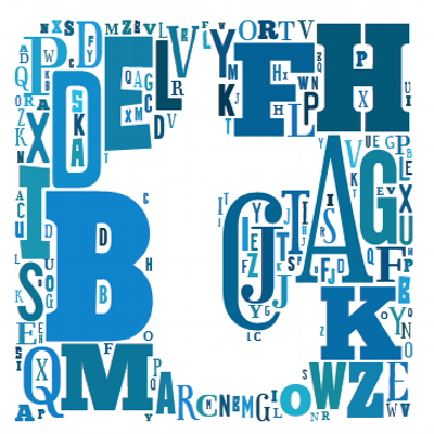
Here is a mind map highlighting how you can turn words into images to create a visual representation of the word, when mindmapping. A simple, yet effective idea illustrating part or all of a word. You can draw “parts” of words, by noticing words within words, or connecting, by imagination, an alternative image from a similar meaning.
Examples include:
Worldwide – flattening the globe comes to mind
Combat – has a comb and a bat or both
Websites – perhaps use eyes looking at a spiders web
Business – has a bus
Legacy – the leg sticks out here!
Organisation – an alternative way to represent this word might include an image of an organ
Seesaw – eyes looking at a saw
Added – taking imagination further you could draw an adder (snake)
Investigate – contains a vest
Flagship – has a flag and a ship
Capture – you might extract the cap and illustrate part of this word
Slim-line – breaking into two words you can represent slim and line
Fundraising – you could illustrate an arm holding a piggybank up in the air
Brain – seeing rain in brain might conjure up an image of a brain, raining thoughts
These words were extracted at random from my files of pencilled mind maps – I chose words that I felt I could demonstrate this idea well with.
This technique is useful particularly when you add a word to a mind map and cannot think how to illustrate it – by breaking down the word and/or considering an alternative meaning you can conjure up new methods of visual representation for the word.
Visual representation allows for humorous associations and gets you thinking in ways that a cartoonist might think, instead of confining yourself strictly to drawing the normal expected version of a word.
See also:
Visual Communication Mind Map
Why I feel Visual Thinking Works
|
Submit your review |
|
| Name: | |
| Email: | |
| Review Title: | |
| Rating: |
1 2 3 4 5 |
| Review: | |
| Check this box to confirm you are human. | |
|
Submit
Cancel |
Average rating:
0 reviews
6 minute read
Word Embeddings are one of the most interesting aspects of the Natural Language Processing field. When I first came across them, it was intriguing to see a simple recipe of unsupervised training on a bunch of text yield representations that show signs of syntactic and semantic understanding.
In this post, we will explore a word embedding algorithm called “FastText” that was introduced by Bojanowski et al. and understand how it enhances the Word2Vec algorithm from 2013.
Intuition on Word Representations
Suppose we have the following words and we want to represent them as vectors so that they can be used in Machine Learning models.
Ronaldo, Messi, Dicaprio
A simple idea could be to perform a one-hot encoding of the words, where each word gets a unique position.
| isRonaldo | isMessi | isDicaprio | |
|---|---|---|---|
| Ronaldo | 1 | 0 | 0 |
| Messi | 0 | 1 | 0 |
| Dicaprio | 0 | 0 | 1 |
We can see that this sparse representation doesn’t capture any relationship between the words and every word is isolated from each other.
Maybe we could do something better. We know Ronaldo and Messi are footballers while Dicaprio is an actor. Let’s use our world knowledge and create manual features to represent the words better.
| isFootballer | isActor | |
|---|---|---|
| Ronaldo | 1 | 0 |
| Messi | 1 | 0 |
| Dicaprio | 0 | 1 |
This is better than the previous one-hot-encoding because related items are closer in space.

We could keep on adding even more aspects as dimensions to get a more nuanced representation.
| isFootballer | isActor | Popularity | Gender | Height | Weight | … | |
|---|---|---|---|---|---|---|---|
| Ronaldo | 1 | 0 | … | … | … | … | … |
| Messi | 1 | 0 | … | … | … | … | … |
| Dicaprio | 0 | 1 | … | … | … | … | … |
But manually doing this for every possible word is not scalable. If we designed features based on our world knowledge of the relationship between words, can we replicate the same with a neural network?
Can we have neural networks comb through a large corpus of text and generate word representations automatically?
This is the intention behind the research in word-embedding algorithms.
Recapping Word2Vec
In 2013, Mikolov et al. introduced an efficient method to learn vector representations of words from large amounts of unstructured text data. The paper was an execution of this idea from Distributional Semantics.
You shall know a word by the company it keeps — J.R. Firth 1957
Since similar words appear in a similar context, Mikolov et al. used this insight to formulate two tasks for representation learning.
The first was called “Continuous Bag of Words” where need to predict the center words given the neighbor words.

The second task was called “Skip-gram” where we need to predict the neighbor words given a center word.

Representations learned had interesting properties such as this popular example where arithmetic operations on word vectors seemed to retain meaning.

Limitations of Word2Vec
While Word2Vec was a game-changer for NLP, we will see how there was still some room for improvement:
-
Out of Vocabulary(OOV) Words:
In Word2Vec, an embedding is created for each word. As such, it can’t handle any words it has not encountered during its training.For example, words such as “tensor” and “flow” are present in the vocabulary of Word2Vec. But if you try to get embedding for the compound word “tensorflow”, you will get an out of vocabulary error.

-
Morphology:
For words with same radicals such as “eat” and “eaten”, Word2Vec doesn’t do any parameter sharing. Each word is learned uniquely based on the context it appears in. Thus, there is scope for utilizing the internal structure of the word to make the process more efficient.


FastText
To solve the above challenges, Bojanowski et al. proposed a new embedding method called FastText. Their key insight was to use the internal structure of a word to improve vector representations obtained from the skip-gram method.
The modification to the skip-gram method is applied as follows:
1. Sub-word generation
For a word, we generate character n-grams of length 3 to 6 present in it.
- We take a word and add angular brackets to denote the beginning and end of a word

-
Then, we generate character n-grams of length n. For example, for the word “eating”, character n-grams of length 3 can be generated by sliding a window of 3 characters from the start of the angular bracket till the ending angular bracket is reached. Here, we shift the window one step each time.
-
Thus, we get a list of character n-grams for a word.
Examples of different length character n-grams are given below:Word Length(n) Character n-grams eating 3 <ea, eat, ati, tin, ing, ng> eating 4 <eat, eati, atin, ting, ing> eating 5 <eati, eatin, ating, ting> eating 6 <eatin, eating, ating> -
Since there can be huge number of unique n-grams, we apply hashing to bound the memory requirements. Instead of learning an embedding for each unique n-gram, we learn total B embeddings where B denotes the bucket size. The paper used a bucket of a size of 2 million.
Each character n-gram is hashed to an integer between 1 to B. Though this could result in collisions, it helps control the vocabulary size. The paper uses the FNV-1a variant of the Fowler-Noll-Vo hashing function to hash character sequences to integer values.


2. Skip-gram with negative sampling
To understand the pre-training, let’s take a simple toy example. We have a sentence with a center word “eating” and need to predict the context words “am” and “food”.

-
First, the embedding for the center word is calculated by taking a sum of vectors for the character n-grams and the whole word itself.
-
For the actual context words, we directly take their word vector from the embedding table without adding the character n-grams.
-
Now, we collect negative samples randomly with probability proportion to the square root of the unigram frequency. For one actual context word, 5 random negative words are sampled.
-
We take dot product between the center word and the actual context words and apply sigmoid function to get a match score between 0 and 1.
-
Based on the loss, we update the embedding vectors with SGD optimizer to bring actual context words closer to the center word but increase distance to the negative samples.


Paper Insights
-
FastText improves performance on syntactic word analogy tasks significantly for morphologically rich language like Czech and German.
word2vec-skipgram word2vec-cbow fasttext Czech 52.8 55.0 77.8 German 44.5 45.0 56.4 English 70.1 69.9 74.9 Italian 51.5 51.8 62.7 -
FastText has degraded performance on semantic analogy tasks compared to Word2Vec.
word2vec-skipgram word2vec-cbow fasttext Czech 25.7 27.6 27.5 German 66.5 66.8 62.3 English 78.5 78.2 77.8 Italian 52.3 54.7 52.3 -
FastText is 1.5 times slower to train than regular skipgram due to added overhead of n-grams.
-
Using sub-word information with character-ngrams has better performance than CBOW and skip-gram baselines on word-similarity task. Representing out-of-vocab words by summing their sub-words has better performance than assigning null vectors.
skipgram cbow fasttext(null OOV) fasttext(char-ngrams for OOV) Arabic WS353 51 52 54 55 GUR350 61 62 64 70 German GUR65 78 78 81 81 ZG222 35 38 41 44 English RW 43 43 46 47 WS353 72 73 71 71 Spanish WS353 57 58 58 59 French RG65 70 69 75 75 Romanian WS353 48 52 51 54 Russian HJ 69 60 60 66


Implementation
To train your own embeddings, you can either use the official CLI tool or use the fasttext implementation available in gensim.
Pre-trained word vectors trained on Common Crawl and Wikipedia for 157 languages are available here and variants of English word vectors are available here.
References
- Piotr Bojanowski et al., “Enriching Word Vectors with Subword Information”
- Armand Joulin et al., “Bag of Tricks for Efficient Text Classification”
- Tomas Mikolov et al., “Efficient Estimation of Word Representations in Vector Space”
Visual Representation of Text Data Sets Using the R tm and wordcloud Packages:  Part One
Douglas M. Wiig


This paper is the next installment in series that examines the use of R scripts to present and analyze complex data sets using various types of visual representations. Previous papers have discussed data sets containing a small number of cases and many variable, and data sets with a large number of cases and  many variables.  The previous tutorials have focused on data sets that were numeric.  In this tutorial I will discuss some uses of the R packages tm and wordcloud to meaningfully display and analyze data sets that are composed of text.  These types of data sets include formal addresses, speeches, web site content, Twitter posts, and many other forms of text based communication.

I will present basic R script to process a text file and display the frequency of significant words contained in the text. The results include a visual display of the words using the size of the font to indicate the relative frequency of the word.  This approach displays increasing font size as specific word frequency increases.  This type of visualization of data is generally referred to as a "wordcloud."  To illustrate the use of this approach I will produce a wordcloud that contains the text from the 2017 Presidental State of the Union Address.

There are generally four steps involved in creating a wordcloud.  The first step involves loading the selected text file and required packages into the R environment.  In the second step the text file is converted into a corpus file type and is cleaned of unwanted text, punctuation and other non-text characters.  The third step involves processing the cleaned file to determine word frequencies, and in the fourth step the wordcloud graphic is created and displayed.

Installing Required Packages

As discussed in previous tutorials I would highly recommend the use of an IDE such as RStudio when composing R scripts.  While it is possible to use the basic editor and package loader that is part of the R distribution, an IDE will give you a wealth of tools for entering, editing, running, and debugging script.  While using RStudio to its fullest potential has a fairly steep learning curve, it is relatively easy to successfully navigate and produce less complex R projects such as this one.

Before moving to the specific code for this project run a list of all of the packages that are loaded when R is started.  If you are using RStudio click on the "Packages" tab in the lower right quadrant of the screen and look through the list of packages.  If you are using the basic R script editor and package loader, at the command prompt use the following command:

#####################################################################################
	>installed.packages()
#####################################################################################

The command produces a list of all currently installed packages.  Depending on the specific R version that you are using the packages for this project may or may not be loaded and available.  I will assume that they will need to be installed. The packages to be loaded are tm, wordcloud, tidyverse, readr, and RColorBrewer.  Use the following code:

#############################################################################
#Load required packages
#############################################################################
install.packages("tm")   #processes data
install.packages("wordcloud")   #creates visual plot
install.packages("tidyverse")   #graphics utilities
install.packages("readr")       #to load text files
install.packages("RColorBrewer") #for color graphics
#############################################################################

Once the packages are installed the raw text file can be loaded.  The complete text of Presidential State of the Union Addresses can be readily accessed on the government web site https://www.govinfo.gov/features/state-of-the-union.  The site has sets of complete text for various years that can be downloaded in several formats.  For this project I used the 2017 State of the Union downloaded in text format.  To load and view the raw text file in the R environment use the "Import Dataset" tab in the upper right quadrant of RStudio or the code below:

#############################################################################
library(readr)
yourdatasetname <- read_table2("path to your data file", col_names = FALSE)
View(dataset)
#############################################################################

 Processing The Data

The goal of this step is to produce the word frequencies that will be used by wordcloud to create the wordcloud graphic display. This process entails converting the raw text file into a corpus format, cleaning the file of unwanted text, converting the cleaned file to a text matrix format, and producing the word frequency counts to be graphed.  The code below accomplishes these tasks.  Follow the comments for a description of each step involved.

 ###########################################################################
 #Take raw text file statu17 and convert to corpus format named docs17
 ###########################################################################
 library(tm)
 docs17 <- Corpus(VectorSource(statu17))
 ###########################################################################
 ###########################################################################
 #Clean punctuation, stopwords, white space
 #Three passes create corpus vector source from original file
 #A corpus is a collection of text
 ###########################################################################
 library(tm)
 library(wordcloud)
 data(docs17)
 docs17 <- tm_map(docs17,removePunctuation) #remove punctuation
 docs17 <- tm_map(docs17,removeWords,stopwords("english"))  #remove stopwords
 docs17 <- tm_map(docs17,stripWhitespace)    #remove white space
 ###########################################################################
 #Cleaned corpus is now formatted into text document matrix
 #Then frequency count done for each word in matrix
 #dmat <-create matrix; dval <-sort; dframe <-count word frequencies
 #docmat <- converts cleaned corpus to text matrix for processing
 ###########################################################################
 docmat <- TermDocumentMatrix(docs17)
 dmat <- as.matrix(docmat)
 dval <- sort(rowSums(dmat),decreasing=TRUE)
 dframe <- data.frame(word=names(dval),freq=dval)
 ###########################################################################

 Once these steps have been completed the data frame "dframe" will now be used by the wordcloud package to produce the graphic.

 Producing the Wordcloud Graphic

We are now ready to produce the graphic plot of word frequencies. The resulting display can be manipulated using a number of settings including color schemes, number of words displayed, size of the wordcloud, minimum word frequency of words to display, and many other factors.  Refer to Appendix B for additional information.

For this project I have chosen to use a white background and a multi-colored word display.  The display is medium size, with 150 words maximum, and a minimum word frequency of two. The resulting graphic is shown in Figure 1. Use the code below to produce and display the wordcloud:


 ##########################################################################################
 #Final step is to use wordcloud to generate graphics
 #There are a number of options that can be set
 #See Appendix for details
 #Use RColorBrewer to generate a color wordcloud
 #RColorBrewer has many options, see Appendix for details
 ##########################################################################################
 library(RColorBrewer)
 set.seed(1234)  #use if random.color=TRUE
 par(bg="white")     #background color
 wordcloud(dframe$word,dframe$freq,colors=brewer.pal(8,"Set1"),random.order=FALSE,
 scale=c(2.75,0.20),min.freq=2,max.words=150,rot.per=0.35)
 ##########################################################################################


As seen above, the wordcloud display is arranged in a manner with the most frequently used words in the largest font at the center of the graph.  As word frequency drops there are somewhat concentric rings of words in smaller and smaller fonts with the smallest font outer rings set by the wordcloud parameter min.freq=2.  At this point I will leave an analysis of the wordcloud to the interpretation of the reader.

In part two of this tutorial I will discuss further use of the wordcloud package to produce comparison wordclouds using SOTU text files from 2017, 2018, 2019, and 2020.  I will also introduce part three of the tutorial which will discuss using wordcloud with very large text data sets such as Twitter posts.

Appendix A: Resources and References

This section contains links and references to resources used in this project.  For further information on specific R packages see the links below.


	Package tm:
	https://cran.r-project.org/web/packages/tm/tm.pdf

	Package RColorBrewer:
	https://cran.r-project.org/web/packages/RColorBrewer/RColorBrewer.pdf

	Package readr:
	https://cran.r-project.org/web/packages/readr/readr.pdf

	Package wordcloud:
	https://cran.r-project.org/web/packages/wordcloud/wordcloud.pdf

	Package tidyverse
	https://cran.r-project.org/web/packages/tidyverse/tidyverse.pdf

	To download the RStudio IDE:
	https://www.rstudio.com/products/rstudio/download

General works relating to R programming:


Robert Kabacoff, R in Action:  Data Analysis and Graphics With R, Sheleter Island, NY:  Manning Publications, 2011.

N.D. Lewis, Visualizing Complex Data in R, N.D. Lewis, 2013.

The text data for the 2017 State of the Union Address was downloaded from:

https://www.govinfo.gov/features/state-of-the-union

Appendix B: R Functions Syntax Usage

This appendix contains the syntax usage for the main R functions used in this paper. See the links in Appendix A for more detail on each function.

readr:
read_table2(file,col_names = TRUE,col_types = NULL,locale = default_locale(),na = "NA",
skip = 0,n_max = Inf,guess_max = min(n_max, 1000),progress = show_progress(),comment = "",
skip_empty_rows = TRUE)

wordcloud:
 wordcloud(words,freq,scale=c(4,.5),min.freq=3,max.words=Inf,
 random.order=TRUE, random.color=FALSE, rot.per=.1,
 colors="black",ordered.colors=FALSE,use.r.layout=FALSE,
 fixed.asp=TRUE, ...)

rcolorbrewer:
 brewer.pal(n, name)
 display.brewer.pal(n, name)
 display.brewer.all(n=NULL, type="all", select=NULL, exact.n=TRUE,colorblindFriendly=FALSE)
 brewer.pal.info

tm:
tm_map(x, FUN, ...)


All R programming for this project was done using RStudio Version 1.2.5033
The PDF version of this document was produced using TeXstudio 2.12.6
Author:  Douglas M. Wiig                                              4/01/2021

Web Site:  http://dmwiig.net

Click the links below to open the PDF version of this post.
Word Clouds
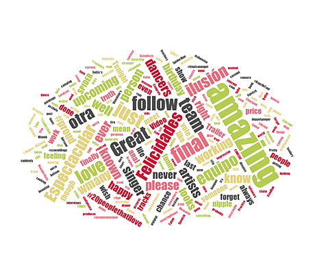
Word Clouds are a visual representation of the frequency of words within a given body of text. Often they are used to visualize the frequency of words within large text documents, qualitative research data, public speeches, website tags, End User License Agreements (EULAs) and unstructured data sources.

Wordclouds.com
Wordclouds.com is a free online word cloud generator and tag cloud creator. Wordclouds.com works on your PC, Tablet or smartphone. Paste text, upload a document or open an URL to automatically generate a word- or tag cloud. Customize your cloud with shapes, themes, colors and fonts. You can also edit the word list, cloud size and gap size. Wordclouds.com can also generate clickable word clouds with links (image map). When you are satisfied with the result, save the image and share it online.

TagCrowd
TagCrowd is a web application for visualizing word frequencies in any text by creating word clouds, and was created by Daniel Steinbock while a PhD student at Stanford University. You can enter text in three ways: paste text, upload a text file or enter the URL of a web page to visualize.
Tagxedo
Tagxedo turns words into a visually stunning word cloud, words individually sized appropriately to highlight the frequencies of occurrence within the body of text. Start with any text and even use images to create a custom shape.
![]()
WordArt
WordArt.com is an online word cloud art creator that enables you to create amazing and unique word cloud art with ease. You can customize every bit of word cloud art including: words, shapes, fonts, colors, layouts and more!

ToCloud
ToCloud is an online free word cloud generator that uses word frequency as the weight. Based on the text from a webpage or pasted text, the generated word cloud of a page gives a quick understanding of how the page is optimized for certain words.

WordItOut
WordItOut is the word cloud generator that gives you control with many custom settings. Free to use and no sign up required!
Word Cloud Generator
Word Cloud Generator is developed by Jason Davies using JavaScript and provides a few customization options for scale, word orientation, font and the number of words from your original text to be included in the word cloud.
![]()
Vizzlo Word Cloud Generator
Vizzlo is an online data visualization tool, and creating word clouds is one of its capabilities. Vizzlo does have offer word cloud creation for free users, but it includes the Vizzlo watermark. You have to be on one of the paid accounts to remove the watermark.
![]()
Word Cloud Maker
Word Cloud Maker is an advanced online FREE word cloud generator that enables you to upload a background photo or select a design from the gallery upon which your word cloud art will be superimposed. You can simply download the word clouds to your local computer in multiple formats such as vector svg, png, jpg, jpeg, pdf and more. You can use it in your content for free.
![]()
Word Cloud Generator (Google Docs)
Word Cloud Generator is a free Google Docs add-on for creating word clouds based on your Google Documents. Richard Byrne has a good video tutorial that demonstrates how to quickly create a word cloud in Google Documents.
![]()
Infogram Word Clouds
Infogram is an online chart maker used to design infographics, presentations, reports and more. It’s free to create an account, and word clouds are one of their charting options. You have to upgrade to a paid plan to remove the Infogram logo and get access to download options for your designs.

WordSift
WordSift was created to help teachers manage the demands of vocabulary and academic language in their text materials. Options are very similar to Jason Davies’ Word Cloud Maker (above) but is easier to use.

MonkeyLearn AI WordCloud Generator
The MonkeyLearn WordCloud Generator is a free tool that uses Artificial Intelligence to generate word clouds from your source text, and automatically detects multiple word combinations.

Wordle (discontinued)
Wordle was a Java-based tool for generating “word clouds” from text that you provide, created by Jonathan Feinberg. Wordle has been discontinued and is no longer under development. You can download and use the final version of the desktop apps for Windows v0.2 and Mac v0.2. These desktop apps require that JAVA is also installed on your computer.