
Присвоение диапазона ячеек объектной переменной в VBA Excel. Адресация ячеек в переменной диапазона и работа с ними. Определение размера диапазона. Примеры.
Присвоение диапазона ячеек переменной
Чтобы переменной присвоить диапазон ячеек, она должна быть объявлена как Variant, Object или Range:
|
Dim myRange1 As Variant Dim myRange2 As Object Dim myRange3 As Range |
Чтобы было понятнее, для чего переменная создана, объявляйте ее как Range.
Присваивается переменной диапазон ячеек с помощью оператора Set:
|
Set myRange1 = Range(«B5:E16») Set myRange2 = Range(Cells(3, 4), Cells(26, 18)) Set myRange3 = Selection |
В выражении Range(Cells(3, 4), Cells(26, 18)) вместо чисел можно использовать переменные.
Для присвоения диапазона ячеек переменной можно использовать встроенное диалоговое окно Application.InputBox, которое позволяет выбрать диапазон на рабочем листе для дальнейшей работы с ним.
Адресация ячеек в диапазоне
К ячейкам присвоенного диапазона можно обращаться по их индексам, а также по индексам строк и столбцов, на пересечении которых они находятся.
Индексация ячеек в присвоенном диапазоне осуществляется слева направо и сверху вниз, например, для диапазона размерностью 5х5:
| 1 | 2 | 3 | 4 | 5 |
| 6 | 7 | 8 | 9 | 10 |
| 11 | 12 | 13 | 14 | 15 |
| 16 | 17 | 18 | 19 | 20 |
| 21 | 22 | 23 | 24 | 25 |
Индексация строк и столбцов начинается с левой верхней ячейки. В диапазоне этого примера содержится 5 строк и 5 столбцов. На пересечении 2 строки и 4 столбца находится ячейка с индексом 9. Обратиться к ней можно так:
|
‘обращение по индексам строки и столбца myRange.Cells(2, 4) ‘обращение по индексу ячейки myRange.Cells(9) |
Обращаться в переменной диапазона можно не только к отдельным ячейкам, но и к части диапазона (поддиапазону), присвоенного переменной, например,
обращение к первой строке присвоенного диапазона размерностью 5х5:
|
myRange.Range(«A1:E1») ‘или myRange.Range(Cells(1, 1), Cells(1, 5)) |
и обращение к первому столбцу присвоенного диапазона размерностью 5х5:
|
myRange.Range(«A1:A5») ‘или myRange.Range(Cells(1, 1), Cells(5, 1)) |
Работа с диапазоном в переменной
Работать с диапазоном в переменной можно точно также, как и с диапазоном на рабочем листе. Все свойства и методы объекта Range действительны и для диапазона, присвоенного переменной. При обращении к ячейке без указания свойства по умолчанию возвращается ее значение. Строки
|
MsgBox myRange.Cells(6) MsgBox myRange.Cells(6).Value |
равнозначны. В обоих случаях информационное сообщение MsgBox выведет значение ячейки с индексом 6.
Важно: если вы планируете работать только со значениями, используйте переменные массивов, код в них работает значительно быстрее.
Преимущество работы с диапазоном ячеек в объектной переменной заключается в том, что все изменения, внесенные в переменной, применяются к диапазону (который присвоен переменной) на рабочем листе.
Пример 1 — работа со значениями
Скопируйте процедуру в программный модуль и запустите ее выполнение.
|
1 2 3 4 5 6 7 8 9 10 11 12 13 14 15 16 17 18 19 20 21 22 23 24 25 |
Sub Test1() ‘Объявляем переменную Dim myRange As Range ‘Присваиваем диапазон ячеек Set myRange = Range(«C6:E8») ‘Заполняем первую строку ‘Присваиваем значение первой ячейке myRange.Cells(1, 1) = 5 ‘Присваиваем значение второй ячейке myRange.Cells(1, 2) = 10 ‘Присваиваем третьей ячейке ‘значение выражения myRange.Cells(1, 3) = myRange.Cells(1, 1) _ * myRange.Cells(1, 2) ‘Заполняем вторую строку myRange.Cells(2, 1) = 20 myRange.Cells(2, 2) = 25 myRange.Cells(2, 3) = myRange.Cells(2, 1) _ + myRange.Cells(2, 2) ‘Заполняем третью строку myRange.Cells(3, 1) = «VBA» myRange.Cells(3, 2) = «Excel» myRange.Cells(3, 3) = myRange.Cells(3, 1) _ & » « & myRange.Cells(3, 2) End Sub |
Обратите внимание, что ячейки диапазона на рабочем листе заполнились так же, как и ячейки в переменной диапазона, что доказывает их непосредственную связь между собой.
Пример 2 — работа с форматами
Продолжаем работу с тем же диапазоном рабочего листа «C6:E8»:
|
Sub Test2() ‘Объявляем переменную Dim myRange As Range ‘Присваиваем диапазон ячеек Set myRange = Range(«C6:E8») ‘Первую строку выделяем жирным шрифтом myRange.Range(«A1:C1»).Font.Bold = True ‘Вторую строку выделяем фоном myRange.Range(«A2:C2»).Interior.Color = vbGreen ‘Третьей строке добавляем границы myRange.Range(«A3:C3»).Borders.LineStyle = True End Sub |
Опять же, обратите внимание, что все изменения форматов в присвоенном диапазоне отобразились на рабочем листе, несмотря на то, что мы непосредственно с ячейками рабочего листа не работали.
Пример 3 — копирование и вставка диапазона из переменной
Значения ячеек диапазона, присвоенного переменной, передаются в другой диапазон рабочего листа с помощью оператора присваивания.
Скопировать и вставить диапазон полностью со значениями и форматами можно при помощи метода Copy, указав место вставки (ячейку) на рабочем листе.
В примере используется тот же диапазон, что и в первых двух, так как он уже заполнен значениями и форматами.
|
1 2 3 4 5 6 7 8 9 10 11 12 13 14 15 16 17 18 |
Sub Test3() ‘Объявляем переменную Dim myRange As Range ‘Присваиваем диапазон ячеек Set myRange = Range(«C6:E8») ‘Присваиваем ячейкам рабочего листа ‘значения ячеек переменной диапазона Range(«A1:C3») = myRange.Value MsgBox «Пауза» ‘Копирование диапазона переменной ‘и вставка его на рабочий лист ‘с указанием начальной ячейки myRange.Copy Range(«E1») MsgBox «Пауза» ‘Копируем и вставляем часть ‘диапазона из переменной myRange.Range(«A2:C2»).Copy Range(«E11») End Sub |
Информационное окно MsgBox добавлено, чтобы вы могли увидеть работу процедуры поэтапно, если решите проверить ее в своей книге Excel.
Размер диапазона в переменной
При получении диапазона с помощью метода Application.InputBox и присвоении его переменной диапазона, бывает полезно узнать его размерность. Это можно сделать следующим образом:
|
Sub Test4() ‘Объявляем переменную Dim myRange As Range ‘Присваиваем диапазон ячеек Set myRange = Application.InputBox(«Выберите диапазон ячеек:», , , , , , , 8) ‘Узнаем количество строк и столбцов MsgBox «Количество строк = « & myRange.Rows.Count _ & vbNewLine & «Количество столбцов = « & myRange.Columns.Count End Sub |
Запустите процедуру, выберите на рабочем листе Excel любой диапазон и нажмите кнопку «OK». Информационное сообщение выведет количество строк и столбцов в диапазоне, присвоенном переменной myRange.
“It is a capital mistake to theorize before one has data”- Sir Arthur Conan Doyle
This post covers everything you need to know about using Cells and Ranges in VBA. You can read it from start to finish as it is laid out in a logical order. If you prefer you can use the table of contents below to go to a section of your choice.
Topics covered include Offset property, reading values between cells, reading values to arrays and formatting cells.
A Quick Guide to Ranges and Cells
| Function | Takes | Returns | Example | Gives |
|---|---|---|---|---|
|
Range |
cell address | multiple cells | .Range(«A1:A4») | $A$1:$A$4 |
| Cells | row, column | one cell | .Cells(1,5) | $E$1 |
| Offset | row, column | multiple cells | Range(«A1:A2») .Offset(1,2) |
$C$2:$C$3 |
| Rows | row(s) | one or more rows | .Rows(4) .Rows(«2:4») |
$4:$4 $2:$4 |
| Columns | column(s) | one or more columns | .Columns(4) .Columns(«B:D») |
$D:$D $B:$D |
Download the Code
The Webinar
If you are a member of the VBA Vault, then click on the image below to access the webinar and the associated source code.
(Note: Website members have access to the full webinar archive.)

Introduction
This is the third post dealing with the three main elements of VBA. These three elements are the Workbooks, Worksheets and Ranges/Cells. Cells are by far the most important part of Excel. Almost everything you do in Excel starts and ends with Cells.
Generally speaking, you do three main things with Cells
- Read from a cell.
- Write to a cell.
- Change the format of a cell.
Excel has a number of methods for accessing cells such as Range, Cells and Offset.These can cause confusion as they do similar things and can lead to confusion
In this post I will tackle each one, explain why you need it and when you should use it.
Let’s start with the simplest method of accessing cells – using the Range property of the worksheet.
Important Notes
I have recently updated this article so that is uses Value2.
You may be wondering what is the difference between Value, Value2 and the default:
' Value2
Range("A1").Value2 = 56

' Value
Range("A1").Value = 56

' Default uses value
Range("A1") = 56
Using Value may truncate number if the cell is formatted as currency. If you don’t use any property then the default is Value.
It is better to use Value2 as it will always return the actual cell value(see this article from Charle Williams.)
The Range Property
The worksheet has a Range property which you can use to access cells in VBA. The Range property takes the same argument that most Excel Worksheet functions take e.g. “A1”, “A3:C6” etc.
The following example shows you how to place a value in a cell using the Range property.
' https://excelmacromastery.com/
Public Sub WriteToCell()

    ' Write number to cell A1 in sheet1 of this workbook
    ThisWorkbook.Worksheets("Sheet1").Range("A1").Value2 = 67

    ' Write text to cell A2 in sheet1 of this workbook
    ThisWorkbook.Worksheets("Sheet1").Range("A2").Value2 = "John Smith"

    ' Write date to cell A3 in sheet1 of this workbook
    ThisWorkbook.Worksheets("Sheet1").Range("A3").Value2 = #11/21/2017#

End Sub
As you can see Range is a member of the worksheet which in turn is a member of the Workbook. This follows the same hierarchy as in Excel so should be easy to understand. To do something with Range you must first specify the workbook and worksheet it belongs to.
For the rest of this post I will use the code name to reference the worksheet.

The following code shows the above example using the code name of the worksheet i.e. Sheet1 instead of ThisWorkbook.Worksheets(“Sheet1”).
' https://excelmacromastery.com/
Public Sub UsingCodeName()

    ' Write number to cell A1 in sheet1 of this workbook
    Sheet1.Range("A1").Value2 = 67

    ' Write text to cell A2 in sheet1 of this workbook
    Sheet1.Range("A2").Value2 = "John Smith"

    ' Write date to cell A3 in sheet1 of this workbook
    Sheet1.Range("A3").Value2 = #11/21/2017#

End Sub
You can also write to multiple cells using the Range property
' https://excelmacromastery.com/
Public Sub WriteToMulti()

    ' Write number to a range of cells
    Sheet1.Range("A1:A10").Value2 = 67

    ' Write text to multiple ranges of cells
    Sheet1.Range("B2:B5,B7:B9").Value2 = "John Smith"

End Sub
You can download working examples of all the code from this post from the top of this article.
The Cells Property of the Worksheet
The worksheet object has another property called Cells which is very similar to range. There are two differences
- Cells returns a range of one cell only.
- Cells takes row and column as arguments.
The example below shows you how to write values to cells using both the Range and Cells property
' https://excelmacromastery.com/
Public Sub UsingCells()

    ' Write to A1
    Sheet1.Range("A1").Value2 = 10
    Sheet1.Cells(1, 1).Value2  = 10

    ' Write to A10
    Sheet1.Range("A10").Value2 = 10
    Sheet1.Cells(10, 1).Value2  = 10

    ' Write to E1
    Sheet1.Range("E1").Value2 = 10
    Sheet1.Cells(1, 5).Value2  = 10

End Sub
You may be wondering when you should use Cells and when you should use Range. Using Range is useful for accessing the same cells each time the Macro runs.
For example, if you were using a Macro to calculate a total and write it to cell A10 every time then Range would be suitable for this task.
Using the Cells property is useful if you are accessing a cell based on a number that may vary. It is easier to explain this with an example.
In the following code, we ask the user to specify the column number. Using Cells gives us the flexibility to use a variable number for the column.
' https://excelmacromastery.com/
Public Sub WriteToColumn()

    Dim UserCol As Integer

    ' Get the column number from the user
    UserCol = Application.InputBox(" Please enter the column...", Type:=1)

    ' Write text to user selected column
    Sheet1.Cells(1, UserCol).Value2 = "John Smith"

End Sub
In the above example, we are using a number for the column rather than a letter.
To use Range here would require us to convert these values to the letter/number cell reference e.g. “C1”. Using the Cells property allows us to provide a row and a column number to access a cell.
Sometimes you may want to return more than one cell using row and column numbers. The next section shows you how to do this.
Using Cells and Range together
As you have seen you can only access one cell using the Cells property. If you want to return a range of cells then you can use Cells with Ranges as follows
' https://excelmacromastery.com/
Public Sub UsingCellsWithRange()

    With Sheet1
        ' Write 5 to Range A1:A10 using Cells property
        .Range(.Cells(1, 1), .Cells(10, 1)).Value2 = 5

        ' Format Range B1:Z1 to be bold
        .Range(.Cells(1, 2), .Cells(1, 26)).Font.Bold = True

    End With

End Sub
As you can see, you provide the start and end cell of the Range. Sometimes it can be tricky to see which range you are dealing with when the value are all numbers. Range has a property called Address which displays the letter/ number cell reference of any range. This can come in very handy when you are debugging or writing code for the first time.
In the following example we print out the address of the ranges we are using:
' https://excelmacromastery.com/
Public Sub ShowRangeAddress()

    ' Note: Using underscore allows you to split up lines of code
    With Sheet1

        ' Write 5 to Range A1:A10 using Cells property
        .Range(.Cells(1, 1), .Cells(10, 1)).Value2 = 5
        Debug.Print "First address is : " _
            + .Range(.Cells(1, 1), .Cells(10, 1)).Address

        ' Format Range B1:Z1 to be bold
        .Range(.Cells(1, 2), .Cells(1, 26)).Font.Bold = True
        Debug.Print "Second address is : " _
            + .Range(.Cells(1, 2), .Cells(1, 26)).Address

    End With

End Sub
In the example I used Debug.Print to print to the Immediate Window. To view this window select View->Immediate Window(or Ctrl G)


You can download all the code for this post from the top of this article.
The Offset Property of Range
Range has a property called Offset. The term Offset refers to a count from the original position. It is used a lot in certain areas of programming. With the Offset property you can get a Range of cells the same size and a certain distance from the current range. The reason this is useful is that sometimes you may want to select a Range based on a certain condition. For example in the screenshot below there is a column for each day of the week. Given the day number(i.e. Monday=1, Tuesday=2 etc.) we need to write the value to the correct column.

We will first attempt to do this without using Offset.
' https://excelmacromastery.com/
' This sub tests with different values
Public Sub TestSelect()

    ' Monday
    SetValueSelect 1, 111.21
    ' Wednesday
    SetValueSelect 3, 456.99
    ' Friday
    SetValueSelect 5, 432.25
    ' Sunday
    SetValueSelect 7, 710.17

End Sub

' Writes the value to a column based on the day
Public Sub SetValueSelect(lDay As Long, lValue As Currency)

    Select Case lDay
        Case 1: Sheet1.Range("H3").Value2 = lValue
        Case 2: Sheet1.Range("I3").Value2 = lValue
        Case 3: Sheet1.Range("J3").Value2 = lValue
        Case 4: Sheet1.Range("K3").Value2 = lValue
        Case 5: Sheet1.Range("L3").Value2 = lValue
        Case 6: Sheet1.Range("M3").Value2 = lValue
        Case 7: Sheet1.Range("N3").Value2 = lValue
    End Select

End Sub
As you can see in the example, we need to add a line for each possible option. This is not an ideal situation. Using the Offset Property provides a much cleaner solution
' https://excelmacromastery.com/
' This sub tests with different values
Public Sub TestOffset()

    DayOffSet 1, 111.01
    DayOffSet 3, 456.99
    DayOffSet 5, 432.25
    DayOffSet 7, 710.17

End Sub

Public Sub DayOffSet(lDay As Long, lValue As Currency)

    ' We use the day value with offset specify the correct column
    Sheet1.Range("G3").Offset(, lDay).Value2 = lValue

End Sub
As you can see this solution is much better. If the number of days in increased then we do not need to add any more code. For Offset to be useful there needs to be some kind of relationship between the positions of the cells. If the Day columns in the above example were random then we could not use Offset. We would have to use the first solution.
One thing to keep in mind is that Offset retains the size of the range. So .Range(“A1:A3”).Offset(1,1) returns the range B2:B4. Below are some more examples of using Offset
' https://excelmacromastery.com/
Public Sub UsingOffset()

    ' Write to B2 - no offset
    Sheet1.Range("B2").Offset().Value2 = "Cell B2"

    ' Write to C2 - 1 column to the right
    Sheet1.Range("B2").Offset(, 1).Value2 = "Cell C2"

    ' Write to B3 - 1 row down
    Sheet1.Range("B2").Offset(1).Value2 = "Cell B3"

    ' Write to C3 - 1 column right and 1 row down
    Sheet1.Range("B2").Offset(1, 1).Value2 = "Cell C3"

    ' Write to A1 - 1 column left and 1 row up
    Sheet1.Range("B2").Offset(-1, -1).Value2 = "Cell A1"

    ' Write to range E3:G13 - 1 column right and 1 row down
    Sheet1.Range("D2:F12").Offset(1, 1).Value2 = "Cells E3:G13"

End Sub
Using the Range CurrentRegion
CurrentRegion returns a range of all the adjacent cells to the given range.
In the screenshot below you can see the two current regions. I have added borders to make the current regions clear.

A row or column of blank cells signifies the end of a current region.
You can manually check the CurrentRegion in Excel by selecting a range and pressing Ctrl + Shift + *.
If we take any range of cells within the border and apply CurrentRegion, we will get back the range of cells in the entire area.
For example
Range(“B3”).CurrentRegion will return the range B3:D14
Range(“D14”).CurrentRegion will return the range B3:D14
Range(“C8:C9”).CurrentRegion will return the range B3:D14
and so on
How to Use
We get the CurrentRegion as follows
' Current region will return B3:D14 from above example
Dim rg As Range
Set rg = Sheet1.Range("B3").CurrentRegion
Read Data Rows Only
Read through the range from the second row i.e.skipping the header row
' Current region will return B3:D14 from above example
Dim rg As Range
Set rg = Sheet1.Range("B3").CurrentRegion

' Start at row 2 - row after header
Dim i As Long
For i = 2 To rg.Rows.Count
    ' current row, column 1 of range
    Debug.Print rg.Cells(i, 1).Value2
Next i
Remove Header
Remove header row(i.e. first row) from the range. For example if range is A1:D4 this will return A2:D4
' Current region will return B3:D14 from above example
Dim rg As Range
Set rg = Sheet1.Range("B3").CurrentRegion

' Remove Header
Set rg = rg.Resize(rg.Rows.Count - 1).Offset(1)

' Start at row 1 as no header row
Dim i As Long
For i = 1 To rg.Rows.Count
    ' current row, column 1 of range
    Debug.Print rg.Cells(i, 1).Value2
Next i
Using Rows and Columns as Ranges
If you want to do something with an entire Row or Column you can use the Rows or Columns property of the Worksheet. They both take one parameter which is the row or column number you wish to access
' https://excelmacromastery.com/
Public Sub UseRowAndColumns()

    ' Set the font size of column B to 9
    Sheet1.Columns(2).Font.Size = 9

    ' Set the width of columns D to F
    Sheet1.Columns("D:F").ColumnWidth = 4

    ' Set the font size of row 5 to 18
    Sheet1.Rows(5).Font.Size = 18

End Sub
Using Range in place of Worksheet
You can also use Cells, Rows and Columns as part of a Range rather than part of a Worksheet. You may have a specific need to do this but otherwise I would avoid the practice. It makes the code more complex. Simple code is your friend. It reduces the possibility of errors.
The code below will set the second column of the range to bold. As the range has only two rows the entire column is considered B1:B2
' https://excelmacromastery.com/
Public Sub UseColumnsInRange()

    ' This will set B1 and B2 to be bold
    Sheet1.Range("A1:C2").Columns(2).Font.Bold = True

End Sub
You can download all the code for this post from the top of this article.
Reading Values from one Cell to another
In most of the examples so far we have written values to a cell. We do this by placing the range on the left of the equals sign and the value to place in the cell on the right. To write data from one cell to another we do the same. The destination range goes on the left and the source range goes on the right.
The following example shows you how to do this:
' https://excelmacromastery.com/
Public Sub ReadValues()

    ' Place value from B1 in A1
    Sheet1.Range("A1").Value2 = Sheet1.Range("B1").Value2

    ' Place value from B3 in sheet2 to cell A1
    Sheet1.Range("A1").Value2 = Sheet2.Range("B3").Value2

    ' Place value from B1 in cells A1 to A5
    Sheet1.Range("A1:A5").Value2 = Sheet1.Range("B1").Value2

    ' You need to use the "Value" property to read multiple cells
    Sheet1.Range("A1:A5").Value2 = Sheet1.Range("B1:B5").Value2

End Sub
As you can see from this example it is not possible to read from multiple cells. If you want to do this you can use the Copy function of Range with the Destination parameter
' https://excelmacromastery.com/
Public Sub CopyValues()

    ' Store the copy range in a variable
    Dim rgCopy As Range
    Set rgCopy = Sheet1.Range("B1:B5")

    ' Use this to copy from more than one cell
    rgCopy.Copy Destination:=Sheet1.Range("A1:A5")

    ' You can paste to multiple destinations
    rgCopy.Copy Destination:=Sheet1.Range("A1:A5,C2:C6")

End Sub
The Copy function copies everything including the format of the cells. It is the same result as manually copying and pasting a selection. You can see more about it in the Copying and Pasting Cells section.
Using the Range.Resize Method
When copying from one range to another using assignment(i.e. the equals sign), the destination range must be the same size as the source range.
Using the Resize function allows us to resize a range to a given number of rows and columns.
For example:
' https://excelmacromastery.com/
Sub ResizeExamples()

    ' Prints A1
    Debug.Print Sheet1.Range("A1").Address

    ' Prints A1:A2
    Debug.Print Sheet1.Range("A1").Resize(2, 1).Address

    ' Prints A1:A5
    Debug.Print Sheet1.Range("A1").Resize(5, 1).Address

    ' Prints A1:D1
    Debug.Print Sheet1.Range("A1").Resize(1, 4).Address

    ' Prints A1:C3
    Debug.Print Sheet1.Range("A1").Resize(3, 3).Address

End Sub
When we want to resize our destination range we can simply use the source range size.
In other words, we use the row and column count of the source range as the parameters for resizing:
' https://excelmacromastery.com/
Sub Resize()

    Dim rgSrc As Range, rgDest As Range

    ' Get all the data in the current region
    Set rgSrc = Sheet1.Range("A1").CurrentRegion

      ' Get the range destination
    Set rgDest = Sheet2.Range("A1")
    Set rgDest = rgDest.Resize(rgSrc.Rows.Count, rgSrc.Columns.Count)

    rgDest.Value2 = rgSrc.Value2

End Sub
We can do the resize in one line if we prefer:
' https://excelmacromastery.com/
Sub ResizeOneLine()

    Dim rgSrc As Range

    ' Get all the data in the current region
    Set rgSrc = Sheet1.Range("A1").CurrentRegion

    With rgSrc
        Sheet2.Range("A1").Resize(.Rows.Count, .Columns.Count).Value2 = .Value2
    End With

End Sub
Reading Values to variables
We looked at how to read from one cell to another. You can also read from a cell to a variable. A variable is used to store values while a Macro is running. You normally do this when you want to manipulate the data before writing it somewhere. The following is a simple example using a variable. As you can see the value of the item to the right of the equals is written to the item to the left of the equals.
' https://excelmacromastery.com/
Public Sub UseVariables()

    ' Create
    Dim number As Long

    ' Read number from cell
    number = Sheet1.Range("A1").Value2

    ' Add 1 to value
    number = number + 1

    ' Write new value to cell
    Sheet1.Range("A2").Value2 = number

End Sub
To read text to a variable you use a variable of type String:
' https://excelmacromastery.com/
Public Sub UseVariableText()

    ' Declare a variable of type string
    Dim text As String

    ' Read value from cell
    text = Sheet1.Range("A1").Value2

    ' Write value to cell
    Sheet1.Range("A2").Value2 = text

End Sub
You can write a variable to a range of cells. You just specify the range on the left and the value will be written to all cells in the range.
' https://excelmacromastery.com/
Public Sub VarToMulti()

    ' Read value from cell
    Sheet1.Range("A1:B10").Value2 = 66

End Sub
You cannot read from multiple cells to a variable. However you can read to an array which is a collection of variables. We will look at doing this in the next section.
How to Copy and Paste Cells
If you want to copy and paste a range of cells then you do not need to select them. This is a common error made by new VBA users.
Note: We normally use Range.Copy when we want to copy formats, formulas, validation. If we want to copy values it is not the most efficient method.
I have written a complete guide to copying data in Excel VBA here.
You can simply copy a range of cells like this:
Range("A1:B4").Copy Destination:=Range("C5")
Using this method copies everything – values, formats, formulas and so on. If you want to copy individual items you can use the PasteSpecial property of range.
It works like this
Range("A1:B4").Copy
Range("F3").PasteSpecial Paste:=xlPasteValues
Range("F3").PasteSpecial Paste:=xlPasteFormats
Range("F3").PasteSpecial Paste:=xlPasteFormulas
The following table shows a full list of all the paste types
| Paste Type |
|---|
| xlPasteAll |
| xlPasteAllExceptBorders |
| xlPasteAllMergingConditionalFormats |
| xlPasteAllUsingSourceTheme |
| xlPasteColumnWidths |
| xlPasteComments |
| xlPasteFormats |
| xlPasteFormulas |
| xlPasteFormulasAndNumberFormats |
| xlPasteValidation |
| xlPasteValues |
| xlPasteValuesAndNumberFormats |
Reading a Range of Cells to an Array
You can also copy values by assigning the value of one range to another.
Range("A3:Z3").Value2 = Range("A1:Z1").Value2
The value of range in this example is considered to be a variant array. What this means is that you can easily read from a range of cells to an array. You can also write from an array to a range of cells. If you are not familiar with arrays you can check them out in this post.
The following code shows an example of using an array with a range:
' https://excelmacromastery.com/
Public Sub ReadToArray()

    ' Create dynamic array
    Dim StudentMarks() As Variant

    ' Read 26 values into array from the first row
    StudentMarks = Range("A1:Z1").Value2

    ' Do something with array here

    ' Write the 26 values to the third row
    Range("A3:Z3").Value2 = StudentMarks

End Sub
Keep in mind that the array created by the read is a 2 dimensional array. This is because a spreadsheet stores values in two dimensions i.e. rows and columns
Going through all the cells in a Range
Sometimes you may want to go through each cell one at a time to check value.
You can do this using a For Each loop shown in the following code
' https://excelmacromastery.com/
Public Sub TraversingCells()

    ' Go through each cells in the range
    Dim rg As Range
    For Each rg In Sheet1.Range("A1:A10,A20")
        ' Print address of cells that are negative
        If rg.Value < 0 Then
            Debug.Print rg.Address + " is negative."
        End If
    Next

End Sub
You can also go through consecutive Cells using the Cells property and a standard For loop.
The standard loop is more flexible about the order you use but it is slower than a For Each loop.
' https://excelmacromastery.com/
Public Sub TraverseCells()

    ' Go through cells from A1 to A10
    Dim i As Long
    For i = 1 To 10
        ' Print address of cells that are negative
        If Range("A" & i).Value < 0 Then
            Debug.Print Range("A" & i).Address + " is negative."
        End If
    Next

    ' Go through cells in reverse i.e. from A10 to A1
    For i = 10 To 1 Step -1
        ' Print address of cells that are negative
        If Range("A" & i) < 0 Then
            Debug.Print Range("A" & i).Address + " is negative."
        End If
    Next

End Sub
Formatting Cells
Sometimes you will need to format the cells the in spreadsheet. This is actually very straightforward. The following example shows you various formatting you can add to any range of cells
' https://excelmacromastery.com/
Public Sub FormattingCells()

    With Sheet1

        ' Format the font
        .Range("A1").Font.Bold = True
        .Range("A1").Font.Underline = True
        .Range("A1").Font.Color = rgbNavy

        ' Set the number format to 2 decimal places
        .Range("B2").NumberFormat = "0.00"
        ' Set the number format to a date
        .Range("C2").NumberFormat = "dd/mm/yyyy"
        ' Set the number format to general
        .Range("C3").NumberFormat = "General"
        ' Set the number format to text
        .Range("C4").NumberFormat = "Text"

        ' Set the fill color of the cell
        .Range("B3").Interior.Color = rgbSandyBrown

        ' Format the borders
        .Range("B4").Borders.LineStyle = xlDash
        .Range("B4").Borders.Color = rgbBlueViolet

    End With

End Sub
Main Points
The following is a summary of the main points
- Range returns a range of cells
- Cells returns one cells only
- You can read from one cell to another
- You can read from a range of cells to another range of cells.
- You can read values from cells to variables and vice versa.
- You can read values from ranges to arrays and vice versa
- You can use a For Each or For loop to run through every cell in a range.
- The properties Rows and Columns allow you to access a range of cells of these types
What’s Next?
Free VBA Tutorial If you are new to VBA or you want to sharpen your existing VBA skills then why not try out the The Ultimate VBA Tutorial.
Related Training: Get full access to the Excel VBA training webinars and all the tutorials.
(NOTE: Planning to build or manage a VBA Application? Learn how to build 10 Excel VBA applications from scratch.)
In this Article
- Ranges and Cells in VBA
- Cell Address
- Range of Cells
- Writing to Cells
- Reading from Cells
- Non Contiguous Cells
- Intersection of Cells
- Offset from a Cell or Range
- Setting Reference to a Range
- Resize a Range
- OFFSET vs Resize
- All Cells in Sheet
- UsedRange
- CurrentRegion
- Range Properties
- Last Cell in Sheet
- Last Used Row Number in a Column
- Last Used Column Number in a Row
- Cell Properties
- Copy and Paste
- AutoFit Contents
- More Range Examples
- For Each
- Sort
- Find
- Range Address
- Range to Array
- Array to Range
- Sum Range
- Count Range
Ranges and Cells in VBA
Excel spreadsheets store data in Cells. Cells are arranged into Rows and Columns. Each cell can be identified by the intersection point of it’s row and column (Exs. B3 or R3C2).
An Excel Range refers to one or more cells (ex. A3:B4)
Cell Address
A1 Notation
In A1 notation, a cell is referred to by it’s column letter (from A to XFD) followed by it’s row number(from 1 to 1,048,576). This is called a cell address.
In VBA you can refer to any cell using the Range Object.
' Refer to cell B4 on the currently active sheet
MsgBox Range("B4")

' Refer to cell B4 on the sheet named 'Data'
MsgBox Worksheets("Data").Range("B4")

' Refer to cell B4 on the sheet named 'Data' in another OPEN workbook
' named 'My Data'
MsgBox Workbooks("My Data").Worksheets("Data").Range("B4")
R1C1 Notation
In R1C1 Notation a cell is referred by R followed by Row Number then letter ‘C’ followed by the Column Number. eg B4 in R1C1 notation will be referred by R4C2. In VBA you use the Cells Object to use R1C1 notation:
' Refer to cell R[6]C[4] i.e D6
Cells(6, 4) = "D6"
Range of Cells
A1 Notation
To refer to a more than one cell use a “:” between the starting cell address and last cell address. The following will refer to all the cells from A1 to D10:
Range("A1:D10")
R1C1 Notation
To refer to a more than one cell use a “,” between the starting cell address and last cell address. The following will refer to all the cells from A1 to D10:
Range(Cells(1, 1), Cells(10, 4))Writing to Cells
To write values to a cell or contiguous group of cells, simple refer to the range, put an = sign and then write the value to be stored:
' Store F5 in cell with Address F6
Range("F6") = "F6"

' Store E6 in cell with Address R[6]C[5] i.e E6
Cells(6, 5) = "E6"

' Store A1:D10 in the range A1:D10
Range("A1:D10") = "A1:D10"
' or
Range(Cells(1, 1), Cells(10, 4)) = "A1:D10"
Reading from Cells
To read values from cells, simple refer to the variable to store the values, put an = sign and then refer to the range to be read:
Dim val1
Dim val2

' Read from cell F6
val1 = Range("F6")

' Read from cell E6
val2 = Cells(6, 5)

MsgBox val1
Msgbox val2
Note: To store values from a range of cells, you need to use an Array instead of a simple variable.
Non Contiguous Cells
To refer to non contiguous cells use a comma between the cell addresses:
' Store 10 in cells A1, A3, and A5
Range("A1,A3,A5") = 10


' Store 10 in cells A1:A3 and D1:D3)
Range("A1:A3, D1:D3") = 10
VBA Coding Made Easy
Stop searching for VBA code online. Learn more about AutoMacro — A VBA Code Builder that allows beginners to code procedures from scratch with minimal coding knowledge and with many time-saving features for all users!

Learn More
Intersection of Cells
To refer to non contiguous cells use a space between the cell addresses:
' Store 'Col D' in D1:D10
' which is Common between A1:D10 and D1:F10
Range("A1:D10 D1:G10") = "Col D"
Offset from a Cell or Range
Using the Offset function, you can move the reference from a given Range (cell or group of cells) by the specified number_of_rows, and number_of_columns.
Offset Syntax
Range.Offset(number_of_rows, number_of_columns)
Offset from a cell
' OFFSET from a cell A1
' Refer to cell itself
' Move 0 rows and 0 columns
Range("A1").Offset(0, 0) = "A1"

' Move 1 rows and 0 columns
Range("A1").Offset(1, 0) = "A2"

' Move 0 rows and 1 columns
Range("A1").Offset(0, 1) = "B1"

' Move 1 rows and 1 columns
Range("A1").Offset(1, 1) = "B2"

' Move 10 rows and 5 columns
Range("A1").Offset(10, 5) = "F11"
Offset from a Range
' Move Reference to Range A1:D4 by 4 rows and 4 columns
' New Reference is E5:H8
Range("A1:D4").Offset(4,4) = "E5:H8"
Setting Reference to a Range
To assign a range to a range variable: declare a variable of type Range then use the Set command to set it to a range. Please note that you must use the SET command as RANGE is an object:
' Declare a Range variable
Dim myRange as Range

' Set the variable to the range A1:D4
Set myRange = Range("A1:D4")

' Prints $A$1:$D$4
MsgBox myRange.Address
VBA Programming | Code Generator does work for you!
Resize a Range
Resize method of Range object changes the dimension of the reference range:
Dim myRange As Range

' Range to Resize
Set myRange = Range("A1:F4")

' Prints $A$1:$E$10
Debug.Print myRange.Resize(10, 5).Address
Top-left cell of the Resized range is same as the top-left cell of the original range
Resize Syntax
Range.Resize(number_of_rows, number_of_columns)
OFFSET vs Resize
Offset does not change the dimensions of the range but moves it by the specified number of rows and columns. Resize does not change the position of the original range but changes the dimensions to the specified number of rows and columns.
All Cells in Sheet
The Cells object refers to all the cells in the sheet (1048576 rows and 16384 columns).
' Clear All Cells in Worksheets
Cells.Clear
UsedRange
UsedRange property gives you the rectangular range from the top-left cell used cell to the right-bottom used cell of the active sheet.
Dim ws As Worksheet
Set ws = ActiveSheet

' $B$2:$L$14 if L2 is the first cell with any value
' and L14 is the last cell with any value on the
' active sheet
Debug.Print ws.UsedRange.Address
CurrentRegion
CurrentRegion property gives you the contiguous rectangular range from the top-left cell to the right-bottom used cell containing the referenced cell/range.
Dim myRange As Range

Set myRange = Range("D4:F6")

' Prints $B$2:$L$14
' If there is a filled path from D4:F16 to B2 AND L14
Debug.Print myRange.CurrentRegion.Address

' You can refer to a single starting cell also

Set myRange = Range("D4") ' Prints $B$2:$L$14
AutoMacro | Ultimate VBA Add-in | Click for Free Trial!
Range Properties
You can get Address, row/column number of a cell, and number of rows/columns in a range as given below:
Dim myRange As Range

Set myRange = Range("A1:F10")

' Prints $A$1:$F$10
Debug.Print myRange.Address

Set myRange = Range("F10")

' Prints 10 for Row 10
Debug.Print myRange.Row

' Prints 6 for Column F
Debug.Print myRange.Column

Set myRange = Range("E1:F5")
' Prints 5 for number of Rows in range
Debug.Print myRange.Rows.Count

' Prints 2 for number of Columns in range
Debug.Print myRange.Columns.Count
Last Cell in Sheet
You can use Rows.Count and Columns.Count properties with Cells object to get the last cell on the sheet:
' Print the last row number
' Prints 1048576
Debug.Print "Rows in the sheet: " & Rows.Count

' Print the last column number
' Prints 16384
Debug.Print "Columns in the sheet: " & Columns.Count

' Print the address of the last cell
' Prints $XFD$1048576
Debug.Print "Address of Last Cell in the sheet: " & Cells(Rows.Count, Columns.Count)
Last Used Row Number in a Column
END property takes you the last cell in the range, and End(xlUp) takes you up to the first used cell from that cell.
Dim lastRow As Long

lastRow = Cells(Rows.Count, "A").End(xlUp).Row
Last Used Column Number in a Row
Dim lastCol As Long

lastCol = Cells(1, Columns.Count).End(xlToLeft).Column
END property takes you the last cell in the range, and End(xlToLeft) takes you left to the first used cell from that cell.
You can also use xlDown and xlToRight properties to navigate to the first bottom or right used cells of the current cell.
AutoMacro | Ultimate VBA Add-in | Click for Free Trial!
Cell Properties
Common Properties
Here is code to display commonly used Cell Properties
Dim cell As Range
Set cell = Range("A1")

cell.Activate
Debug.Print cell.Address
' Print $A$1

Debug.Print cell.Value
' Prints 456
' Address

Debug.Print cell.Formula
' Prints =SUM(C2:C3)

' Comment
Debug.Print cell.Comment.Text

' Style
Debug.Print cell.Style

' Cell Format
Debug.Print cell.DisplayFormat.NumberFormat
Cell Font
Cell.Font object contains properties of the Cell Font:
Dim cell As Range

Set cell = Range("A1")

' Regular, Italic, Bold, and Bold Italic
cell.Font.FontStyle = "Bold Italic"
' Same as
cell.Font.Bold = True
cell.Font.Italic = True

' Set font to Courier
cell.Font.FontStyle = "Courier"

' Set Font Color
cell.Font.Color = vbBlue
' or
cell.Font.Color = RGB(255, 0, 0)

' Set Font Size
cell.Font.Size = 20
Copy and Paste
Paste All
Ranges/Cells can be copied and pasted from one location to another. The following code copies all the properties of source range to destination range (equivalent to CTRL-C and CTRL-V)
'Simple Copy
Range("A1:D20").Copy
Worksheets("Sheet2").Range("B10").Paste

'or
' Copy from Current Sheet to sheet named 'Sheet2'
Range("A1:D20").Copy destination:=Worksheets("Sheet2").Range("B10")
Paste Special
Selected properties of the source range can be copied to the destination by using PASTESPECIAL option:
' Paste the range as Values only
Range("A1:D20").Copy
Worksheets("Sheet2").Range("B10").PasteSpecial Paste:=xlPasteValues
Here are the possible options for the Paste option:
' Paste Special Types
xlPasteAll
xlPasteAllExceptBorders
xlPasteAllMergingConditionalFormats
xlPasteAllUsingSourceTheme
xlPasteColumnWidths
xlPasteComments
xlPasteFormats
xlPasteFormulas
xlPasteFormulasAndNumberFormats
xlPasteValidation
xlPasteValues
xlPasteValuesAndNumberFormats
AutoFit Contents
Size of rows and columns can be changed to fit the contents using AutoFit:
' Change size of rows 1 to 5 to fit contents
Rows("1:5").AutoFit

' Change size of Columns A to B to fit contents
Columns("A:B").AutoFit
More Range Examples
It is recommended that you use Macro Recorder while performing the required action through the GUI. It will help you understand the various options available and how to use them.
AutoMacro | Ultimate VBA Add-in | Click for Free Trial!
For Each
It is easy to loop through a range using For Each construct as show below:
For Each cell In Range("A1:B100")
    ' Do something with the cell
Next cell
At each iteration of the loop one cell in the range is assigned to the variable cell and statements in the For loop are executed for that cell. Loop exits when all the cells are processed.
Sort
Sort is a method of Range object. You can sort a range by specifying options for sorting to Range.Sort. The code below will sort the columns A:C based on key in cell C2. Sort Order can be xlAscending or xlDescending. Header:= xlYes should be used if first row is the header row.
   Columns("A:C").Sort key1:=Range("C2"), _
      order1:=xlAscending, Header:=xlYes
Find
Find is also a method of Range Object. It find the first cell having content matching the search criteria and returns the cell as a Range object. It return Nothing if there is no match.
Use FindNext method (or FindPrevious) to find next(previous) occurrence.
Following code will change the font to “Arial Black” for all cells in the range which start with “John”:
For Each c In Range("A1:A100")
    If c Like "John*" Then
        c.Font.Name = "Arial Black"
    End If
Next c
Following code will replace all occurrences of “To Test” to “Passed” in the range specified:
With Range("a1:a500")
    Set c = .Find("To Test", LookIn:=xlValues)
    If Not c Is Nothing Then
        firstaddress = c.Address
        Do
            c.Value = "Passed"
            Set c = .FindNext(c)
        Loop While Not c Is Nothing And c.Address <> firstaddress
    End If
End With
It is important to note that you must specify a range to use FindNext. Also you must provide a stopping condition otherwise the loop will execute forever. Normally address of the first cell which is found is stored in a variable and loop is stopped when you reach that cell again. You must also check for the case when nothing is found to stop the loop.
Range Address
Use Range.Address to get the address in A1 Style
MsgBox Range("A1:D10").Address
' or
Debug.Print Range("A1:D10").Address
Use xlReferenceStyle (default is xlA1) to get addres in R1C1 style
MsgBox Range("A1:D10").Address(ReferenceStyle:=xlR1C1)
' or
Debug.Print Range("A1:D10").Address(ReferenceStyle:=xlR1C1)
This is useful when you deal with ranges stored in variables and want to process for certain addresses only.
AutoMacro | Ultimate VBA Add-in | Click for Free Trial!
Range to Array
It is faster and easier to transfer a range to an array and then process the values. You should declare the array as Variant to avoid calculating the size required to populate the range in the array. Array’s dimensions are set to match number of values in the range.
Dim DirArray As Variant
' Store the values in the range to the Array

DirArray = Range("a1:a5").Value

' Loop to process the values
For Each c In DirArray
    Debug.Print c
Next
Array to Range
After processing you can write the Array back to a Range. To write the Array in the example above to a Range you must specify a Range whose size matches the number of elements in the Array.
Use the code below to write the Array to the range D1:D5:
Range("D1:D5").Value = DirArray

Range("D1:H1").Value = Application.Transpose(DirArray)
Please note that you must Transpose the Array if you write it to a row.
Sum Range
SumOfRange = Application.WorksheetFunction.Sum(Range("A1:A10"))
Debug.Print SumOfRange
You can use many functions available in Excel in your VBA code by specifying Application.WorkSheetFunction. before the Function Name as in the example above.
Count Range
' Count Number of Cells with Numbers in the Range
CountOfCells = Application.WorksheetFunction.Count(Range("A1:A10"))
Debug.Print CountOfCells

' Count Number of Non Blank Cells in the Range
CountOfNonBlankCells = Application.WorksheetFunction.CountA(Range("A1:A10"))
Debug.Print CountOfNonBlankCells
Written by: Vinamra Chandra
Время на прочтение
7 мин
Количество просмотров 312K
Приветствую всех.
В этом посте я расскажу, что такое VBA и как с ним работать в Microsoft Excel 2007/2010 (для более старых версий изменяется лишь интерфейс — код, скорее всего, будет таким же) для автоматизации различной рутины.

VBA (Visual Basic for Applications) — это упрощенная версия Visual Basic, встроенная в множество продуктов линейки Microsoft Office. Она позволяет писать программы прямо в файле конкретного документа. Вам не требуется устанавливать различные IDE — всё, включая отладчик, уже есть в Excel.
Еще при помощи Visual Studio Tools for Office можно писать макросы на C# и также встраивать их. Спасибо, FireStorm.
Сразу скажу — писать на других языках (C++/Delphi/PHP) также возможно, но требуется научится читать, изменять и писать файлы офиса — встраивать в документы не получится. А интерфейсы Microsoft работают через COM. Чтобы вы поняли весь ужас, вот Hello World с использованием COM.
Поэтому, увы, будем учить Visual Basic.
Чуть-чуть подготовки и постановка задачи
Итак, поехали. Открываем Excel.
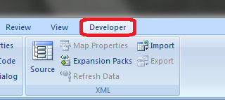
Для начала давайте добавим в Ribbon панель «Разработчик». В ней находятся кнопки, текстовые поля и пр. элементы для конструирования форм.

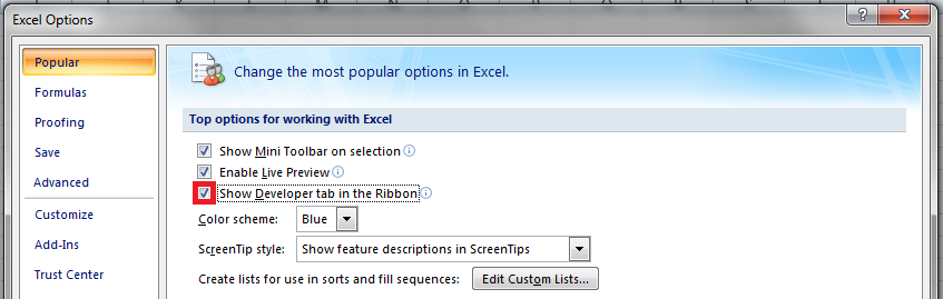
Появилась вкладка.
Теперь давайте подумаем, на каком примере мы будем изучать VBA. Недавно мне потребовалось красиво оформить прайс-лист, выглядевший, как таблица. Идём в гугл, набираем «прайс-лист» и качаем любой, который оформлен примерно так (не сочтите за рекламу, пожалуйста):

То есть требуется, чтобы было как минимум две группы, по которым можно объединить товары (в нашем случае это будут Тип и Производитель — в таком порядке). Для того, чтобы предложенный мною алгоритм работал корректно, отсортируйте товары так, чтобы товары из одной группы стояли подряд (сначала по Типу, потом по Производителю).
Результат, которого хотим добиться, выглядит примерно так:

Разумеется, если смотреть прайс только на компьютере, то можно добавить фильтры и будет гораздо удобнее искать нужный товар. Однако мы хотим научится кодить и задача вполне подходящая, не так ли?
Кодим
Для начала требуется создать кнопку, при нажатии на которую будет вызываться наша програма. Кнопки находятся в панели «Разработчик» и появляются по кнопке «Вставить». Вам нужен компонент формы «Кнопка». Нажали, поставили на любое место в листе. Далее, если не появилось окно назначения макроса, надо нажать правой кнопкой и выбрать пункт «Назначить макрос». Назовём его FormatPrice. Важно, чтобы перед именем макроса ничего не было — иначе он создастся в отдельном модуле, а не в пространстве имен книги. В этому случае вам будет недоступно быстрое обращение к выделенному листу. Нажимаем кнопку «Новый».


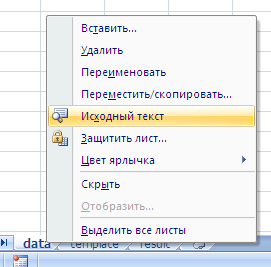
И вот мы в среде разработки VB. Также её можно вызвать из контекстного меню командой «Исходный текст»/«View code».

Перед вами окно с заглушкой процедуры. Можете его развернуть. Код должен выглядеть примерно так:
Sub FormatPrice()End Sub
Напишем Hello World:
Sub FormatPrice()

    MsgBox "Hello World!"

End Sub
И запустим либо щелкнув по кнопке (предварительно сняв с неё выделение), либо клавишей F5 прямо из редактора.
Тут, пожалуй, следует отвлечься на небольшой ликбез по поводу синтаксиса VB. Кто его знает — может смело пропустить этот раздел до конца. Основное отличие Visual Basic от Pascal/C/Java в том, что команды разделяются не ;, а переносом строки или двоеточием (:), если очень хочется написать несколько команд в одну строку. Чтобы понять основные правила синтаксиса, приведу абстрактный код.
Примеры синтаксиса
' Процедура. Ничего не возвращает

' Перегрузка в VBA отсутствует

Sub foo(a As String, b As String)

    ' Exit Sub ' Это значит "выйти из процедуры"

    MsgBox a + ";" + b

End Sub' Функция. Вовращает Integer

Function LengthSqr(x As Integer, y As Integer) As Integer

    ' Exit Function

    LengthSqr = x * x + y * y

End FunctionSub FormatPrice()

    Dim s1 As String, s2 As String

    s1 = "str1"

    s2 = "str2"

    If s1 <> s2 Then

        foo "123", "456" ' Скобки при вызове процедур запрещены

    End IfDim res As sTRING ' Регистр в VB не важен. Впрочем, редактор Вас поправит

    Dim i As Integer

    ' Цикл всегда состоит из нескольких строк

    For i = 1 To 10

        res = res + CStr(i) ' Конвертация чего угодно в String

        If i = 5 Then Exit For

    Next iDim x As Double

    x = Val("1.234") ' Парсинг чисел

    x = x + 10

    MsgBox xOn Error Resume Next ' Обработка ошибок - игнорировать все ошибки

    x = 5 / 0

    MsgBox xOn Error GoTo Err ' При ошибке перейти к метке Err

    x = 5 / 0

    MsgBox "OK!"

    GoTo ne
Err:
MsgBox
"Err!"
ne:
On Error GoTo 0 ' Отключаем обработку ошибок
' Циклы бывает, какие захотите
Do While True
Exit DoLoop 'While True
Do 'Until False
Exit Do
Loop Until False
' А вот при вызове функций, от которых хотим получить значение, скобки нужны.
' Val также умеет возвращать Integer
Select Case LengthSqr(Len("abc"), Val("4"))
Case 24
MsgBox "0"
Case 25
MsgBox "1"
Case 26
MsgBox "2"
End Select' Двухмерный массив.
' Можно также менять размеры командой ReDim (Preserve) - см. google
Dim arr(1 to 10, 5 to 6) As Integer
arr(1, 6) = 8Dim coll As New Collection
Dim coll2 As Collection
coll.Add "item", "key"
Set coll2 = coll ' Все присваивания объектов должны производится командой Set
MsgBox coll2("key")
Set coll2 = New Collection
MsgBox coll2.Count
End Sub
Грабли-1. При копировании кода из IDE (в английском Excel) есь текст конвертируется в 1252 Latin-1. Поэтому, если хотите сохранить русские комментарии — надо сохранить крокозябры как Latin-1, а потом открыть в 1251.
Грабли-2. Т.к. VB позволяет использовать необъявленные переменные, я всегда в начале кода (перед всеми процедурами) ставлю строчку Option Explicit. Эта директива запрещает интерпретатору заводить переменные самостоятельно.
Грабли-3. Глобальные переменные можно объявлять только до первой функции/процедуры. Локальные — в любом месте процедуры/функции.
Еще немного дополнительных функций, которые могут пригодится: InPos, Mid, Trim, LBound, UBound. Также ответы на все вопросы по поводу работы функций/их параметров можно получить в MSDN.
Надеюсь, что этого Вам хватит, чтобы не пугаться кода и самостоятельно написать какое-нибудь домашнее задание по информатике. По ходу поста я буду ненавязчиво знакомить Вас с новыми конструкциями.
Кодим много и под Excel
В этой части мы уже начнём кодить нечто, что умеет работать с нашими листами в Excel. Для начала создадим отдельный лист с именем result (лист с данными назовём data). Теперь, наверное, нужно этот лист очистить от того, что на нём есть. Также мы «выделим» лист с данными, чтобы каждый раз не писать длинное обращение к массиву с листами.
Sub FormatPrice()

    Sheets("result").Cells.Clear

    Sheets("data").Activate

End Sub
Работа с диапазонами ячеек
Вся работа в Excel VBA производится с диапазонами ячеек. Они создаются функцией Range и возвращают объект типа Range. У него есть всё необходимое для работы с данными и/или оформлением. Кстати сказать, свойство Cells листа — это тоже Range.
Примеры работы с Range
Sheets("result").Activate

Dim r As Range

Set r = Range("A1")

r.Value = "123"

Set r = Range("A3,A5")

r.Font.Color = vbRed

r.Value = "456"

Set r = Range("A6:A7")

r.Value = "=A1+A3"
Теперь давайте поймем алгоритм работы нашего кода. Итак, у каждой строчки листа data, начиная со второй, есть некоторые данные, которые нас не интересуют (ID, название и цена) и есть две вложенные группы, к которым она принадлежит (тип и производитель). Более того, эти строки отсортированы. Пока мы забудем про пропуски перед началом новой группы — так будет проще. Я предлагаю такой алгоритм:
- Считали группы из очередной строки.
- Пробегаемся по всем группам в порядке приоритета (вначале более крупные)
- Если текущая группа не совпадает, вызываем процедуру AddGroup(i, name), где i — номер группы (от номера текущей до максимума), name — её имя. Несколько вызовов необходимы, чтобы создать не только наш заголовок, но и всё более мелкие.
- После отрисовки всех необходимых заголовков делаем еще одну строку и заполняем её данными.
Для упрощения работы рекомендую определить следующие функции-сокращения:
Function GetCol(Col As Integer) As String

    GetCol = Chr(Asc("A") + Col)

End FunctionFunction GetCellS(Sheet As String, Col As Integer, Row As Integer) As Range

    Set GetCellS = Sheets(Sheet).Range(GetCol(Col) + CStr(Row))

End FunctionFunction GetCell(Col As Integer, Row As Integer) As Range

    Set GetCell = Range(GetCol(Col) + CStr(Row))

End Function
Далее определим глобальную переменную «текущая строчка»: Dim CurRow As Integer. В начале процедуры её следует сделать равной единице. Еще нам потребуется переменная-«текущая строка в data», массив с именами групп текущей предыдущей строк. Потом можно написать цикл «пока первая ячейка в строке непуста».
Глобальные переменные
Option Explicit ' про эту строчку я уже рассказывал

Dim CurRow As Integer

Const GroupsCount As Integer = 2

Const DataCount As Integer = 3
FormatPrice
Sub FormatPrice()

    Dim I As Integer ' строка в data

    CurRow = 1

    Dim Groups(1 To GroupsCount) As String

    Dim PrGroups(1 To GroupsCount) As String
Sheets(
"data").Activate
I = 2
Do While True
If GetCell(0, I).Value = "" Then Exit Do
' ...
I = I + 1
Loop
End Sub
Теперь надо заполнить массив Groups:
На месте многоточия
Dim I2 As Integer

For I2 = 1 To GroupsCount

    Groups(I2) = GetCell(I2, I)

Next I2

' ...

For I2 = 1 To GroupsCount ' VB не умеет копировать массивы

    PrGroups(I2) = Groups(I2)

Next I2

I =  I + 1
И создать заголовки:
На месте многоточия в предыдущем куске
For I2 = 1 To GroupsCount

    If Groups(I2) <> PrGroups(I2) Then

        Dim I3 As Integer

        For I3 = I2 To GroupsCount

            AddHeader I3, Groups(I3)

        Next I3

        Exit For

    End If

Next I2
Не забудем про процедуру AddHeader:
Перед FormatPrice
Sub AddHeader(Ty As Integer, Name As String)

    GetCellS("result", 1, CurRow).Value = Name

    CurRow = CurRow + 1

End Sub
Теперь надо перенести всякую информацию в result
For I2 = 0 To DataCount - 1

    GetCellS("result", I2, CurRow).Value = GetCell(I2, I)

Next I2
Подогнать столбцы по ширине и выбрать лист result для показа результата
После цикла в конце FormatPrice
Sheets("Result").Activate

Columns.AutoFit
Всё. Можно любоваться первой версией.

Некрасиво, но похоже. Давайте разбираться с форматированием. Сначала изменим процедуру AddHeader:
Sub AddHeader(Ty As Integer, Name As String)

    Sheets("result").Range("A" + CStr(CurRow) + ":C" + CStr(CurRow)).Merge

    ' Чтобы не заводить переменную и не писать каждый раз длинный вызов

    ' можно воспользоваться блоком With

    With GetCellS("result", 0, CurRow)

        .Value = Name

        .Font.Italic = True

        .Font.Name = "Cambria"

        Select Case Ty

        Case 1 ' Тип

            .Font.Bold = True

            .Font.Size = 16

        Case 2 ' Производитель

            .Font.Size = 12

        End Select

        .HorizontalAlignment = xlCenter

    End With

    CurRow = CurRow + 1

End Sub
Уже лучше:

Осталось только сделать границы. Тут уже нам требуется работать со всеми объединёнными ячейками, иначе бордюр будет только у одной:

Поэтому чуть-чуть меняем код с добавлением стиля границ:
Sub AddHeader(Ty As Integer, Name As String)

    With Sheets("result").Range("A" + CStr(CurRow) + ":C" + CStr(CurRow))

        .Merge

        .Value = Name

        .Font.Italic = True

        .Font.Name = "Cambria"

        .HorizontalAlignment = xlCenterSelect Case Ty

        Case 1 ' Тип

            .Font.Bold = True

            .Font.Size = 16

            .Borders(xlTop).Weight = xlThick

        Case 2 ' Производитель

            .Font.Size = 12

            .Borders(xlTop).Weight = xlMedium

        End Select

        .Borders(xlBottom).Weight = xlMedium ' По убыванию: xlThick, xlMedium, xlThin, xlHairline

    End With

    CurRow = CurRow + 1

End Sub

Осталось лишь добится пропусков перед началом новой группы. Это легко:
В начале FormatPrice
Dim I As Integer ' строка в  data

CurRow = 0 ' чтобы не было пропуска в самом начале

Dim Groups(1 To GroupsCount) As String
В цикле расстановки заголовков
If Groups(I2) <> PrGroups(I2) Then

    CurRow = CurRow + 1

    Dim I3 As Integer

В точности то, что и хотели.
Надеюсь, что эта статья помогла вам немного освоится с программированием для Excel на VBA. Домашнее задание — добавить заголовки «ID, Название, Цена» в результат. Подсказка: CurRow = 0 CurRow = 1.
Файл можно скачать тут (min.us) или тут (Dropbox). Не забудьте разрешить исполнение макросов. Если кто-нибудь подскажет человеческих файлохостинг, залью туда.
Спасибо за внимание.
Буду рад конструктивной критике в комментариях.
UPD: Перезалил пример на Dropbox и min.us.
UPD2: На самом деле, при вызове процедуры с одним параметром скобки можно поставить. Либо использовать конструкцию Call Foo(«bar», 1, 2, 3) — тут скобки нужны постоянно.
Синтаксис
- Set — оператор, используемый для установки ссылки на объект, например, на диапазон
- Для каждого — оператор, используемый для прокрутки каждого элемента в коллекции
замечания
Обратите внимание, что имена переменных r , cell и другие могут быть названы, как вам нравится, но должны быть названы соответствующим образом, чтобы код был более понятным для вас и других.
Создание диапазона
Диапазон нельзя создать или заполнить так же, как строка:
Sub RangeTest()
    Dim s As String
    Dim r As Range 'Specific Type of Object, with members like Address, WrapText, AutoFill, etc.

    ' This is how we fill a String:
    s = "Hello World!"

    ' But we cannot do this for a Range:
    r = Range("A1") '//Run. Err.:  91 Object variable or With block variable not set//

    ' We have to use the Object approach, using keyword Set:
    Set r = Range("A1")
End Sub
Считается лучшей практикой, чтобы квалифицировать ваши ссылки , поэтому в дальнейшем мы будем использовать один и тот же подход.
Подробнее о создании объектных переменных (например, Range) в MSDN . Подробнее о Set Statement на MSDN .
Существуют разные способы создания одного и того же диапазона:
Sub SetRangeVariable()
    Dim ws As Worksheet
    Dim r As Range

    Set ws = ThisWorkbook.Worksheets(1) ' The first Worksheet in Workbook with this code in it

    ' These are all equivalent:
    Set r = ws.Range("A2")
    Set r = ws.Range("A" & 2)
    Set r = ws.Cells(2, 1) ' The cell in row number 2, column number 1
    Set r = ws.[A2] 'Shorthand notation of Range.
    Set r = Range("NamedRangeInA2") 'If the cell A2 is named NamedRangeInA2. Note, that this is Sheet independent.
    Set r = ws.Range("A1").Offset(1, 0) ' The cell that is 1 row and 0 columns away from A1
    Set r = ws.Range("A1").Cells(2,1) ' Similar to Offset. You can "go outside" the original Range.

    Set r = ws.Range("A1:A5").Cells(2) 'Second cell in bigger Range.
    Set r = ws.Range("A1:A5").Item(2) 'Second cell in bigger Range.
    Set r = ws.Range("A1:A5")(2) 'Second cell in bigger Range.
End Sub
Обратите внимание на пример, что ячейки (2, 1) эквивалентны диапазону («A2»). Это происходит потому, что Cells возвращает объект Range.
Некоторые источники: Chip Pearson-Cells Within Ranges ; Объект диапазона MSDN ; John Walkenback — ссылка на диапазоны в коде VBA .
Также обратите внимание, что в любом случае, когда число используется в объявлении диапазона, а сам номер находится вне кавычек, например Range («A» & 2), вы можете поменять это число на переменную, содержащую целое число / долго. Например:
Sub RangeIteration()
    Dim wb As Workbook, ws As Worksheet
    Dim r As Range

    Set wb = ThisWorkbook
    Set ws = wb.Worksheets(1)

    For i = 1 To 10
        Set r = ws.Range("A" & i)
        ' When i = 1, the result will be Range("A1")
        ' When i = 2, the result will be Range("A2")
        ' etc.
        ' Proof:
        Debug.Print r.Address
    Next i
End Sub
Если вы используете двойные циклы, ячейки лучше:
Sub RangeIteration2()
    Dim wb As Workbook, ws As Worksheet
    Dim r As Range

    Set wb = ThisWorkbook
    Set ws = wb.Worksheets(1)

    For i = 1 To 10
        For j = 1 To 10
            Set r = ws.Cells(i, j)
            ' When i = 1 and j = 1, the result will be Range("A1")
            ' When i = 2 and j = 1, the result will be Range("A2")
            ' When i = 1 and j = 2, the result will be Range("B1")
            ' etc.
            ' Proof:
            Debug.Print r.Address
        Next j
    Next i
End Sub
Способы обращения к одной ячейке
Самый простой способ ссылаться на одну ячейку на текущем листе Excel — это просто вставить форму А1 в ссылку в квадратных скобках:
[a3] = "Hello!"
Обратите внимание, что квадратные скобки — это просто удобный синтаксический сахар для метода Evaluate объекта Application , так что технически это идентично следующему коду:
Application.Evaluate("a3") = "Hello!"
Вы также можете вызвать метод Cells который принимает строку и столбец и возвращает ссылку на ячейку.
Cells(3, 1).Formula = "=A1+A2"
Помните, что всякий раз, когда вы передаете строку и столбец в Excel из VBA, строка всегда первая, за ней следует столбец, что запутывает, потому что это противоположно общей нотации A1 где сначала отображается столбец.
В обоих этих примерах мы не указали рабочий лист, поэтому Excel будет использовать активный лист (лист, который находится впереди в пользовательском интерфейсе). Вы можете указать активный лист явно:
ActiveSheet.Cells(3, 1).Formula = "=SUM(A1:A2)"
Или вы можете указать имя определенного листа:
Sheets("Sheet2").Cells(3, 1).Formula = "=SUM(A1:A2)"
Существует множество методов, которые можно использовать для перехода от одного диапазона к другому. Например, метод Rows может использоваться для доступа к отдельным строкам любого диапазона, и метод Cells может использоваться для доступа к отдельным ячейкам строки или столбца, поэтому следующий код относится к ячейке C1:
ActiveSheet.Rows(1).Cells(3).Formula = "hi!"
Сохранение ссылки на ячейку переменной
Чтобы сохранить ссылку на ячейку в переменной, вы должны использовать синтаксис Set , например:
Dim R as Range
Set R = ActiveSheet.Cells(3, 1)
потом…
R.Font.Color = RGB(255, 0, 0)
Почему требуется ключевое слово Set ? Set указывает Visual Basic, что значение в правой части = означает объект.
Смещение недвижимости
- Смещение (строки, столбцы) — оператор, используемый для статической ссылки на другую точку из текущей ячейки. Часто используется в циклах. Следует понимать, что положительные числа в разделе строк перемещаются вправо, поскольку негативы перемещаются влево. С положительными позициями столбцов вниз и негативы двигаются вверх.
т.е.
Private Sub this()
    ThisWorkbook.Sheets("Sheet1").Range("A1").Offset(1, 1).Select
    ThisWorkbook.Sheets("Sheet1").Range("A1").Offset(1, 1).Value = "New Value"
    ActiveCell.Offset(-1, -1).Value = ActiveCell.Value
    ActiveCell.Value = vbNullString
End Sub
Этот код выбирает B2, помещает туда новую строку, затем перемещает эту строку обратно в A1 после очистки B2.
Как перемещать диапазоны (по горизонтали по вертикали и наоборот)
Sub TransposeRangeValues()
    Dim TmpArray() As Variant, FromRange as Range, ToRange as Range

    set FromRange = Sheets("Sheet1").Range("a1:a12")         'Worksheets(1).Range("a1:p1")
    set ToRange = ThisWorkbook.Sheets("Sheet1").Range("a1")  'ThisWorkbook.Sheets("Sheet1").Range("a1")

    TmpArray = Application.Transpose(FromRange.Value)
    FromRange.Clear
    ToRange.Resize(FromRange.Columns.Count,FromRange.Rows.Count).Value2 = TmpArray
End Sub
Примечание. Copy / PasteSpecial также имеет параметр «Вставить транспонирование», который также обновляет формулы транспонированных ячеек.
Хитрости »
27 Июль 2013 307077 просмотров
Полагаю не совру когда скажу, что все кто программирует в VBA очень часто в своих кодах общаются к ячейкам листов. Ведь это чуть ли не основное предназначение VBA в Excel. В принципе ничего сложного в этом нет. Например, чтобы записать в ячейку A1 слово Привет необходимо выполнить код:
Range("A1").Value = "Привет"
Тоже самое можно сделать сразу для нескольких ячеек:
Range("A1:C10").Value = "Привет"
Если необходимо обратиться к именованному диапазону:
Range("Диапазон1").Select
Диапазон1 — это имя диапазона/ячейки, к которому надо обратиться в коде. Указывается в кавычках, как и адреса ячеек.
Но в VBA есть и альтернативный метод записи значений в ячейке — через объект Cells:
Cells(1, 1).Value = "Привет"
Синтаксис объекта Range:
Range(Cell1, Cell2)
- Cell1 — первая ячейка диапазона. Может быть ссылкой на ячейку или диапазон ячеек, текстовым представлением адреса или имени диапазона/ячейки. Допускается указание несвязанных диапазонов(A1,B10), пересечений(A1 B10).
- Cell2 — последняя ячейка диапазона. Необязательна к указанию. Допускается указание ссылки на ячейку, столбец или строку.
Синтаксис объекта Cells:
Cells(Rowindex, Columnindex)
- Rowindex — номер строки
- Columnindex — номер столбца
Исходя из этого несложно предположить, что к диапазону можно обратиться, используя Cells и Range:
'выделяем диапазон "A1:B10" на активном листе
Range(Cells(1,1), Cells(10,2)).Select
и для чего? Ведь можно гораздо короче:
Иногда обращение посредством Cells куда удобнее. Например для цикла по столбцам(да еще и с шагом 3) совершенно неудобно было бы использовать буквенное обозначение столбцов.
Объект Cells так же можно использовать для указания ячеек внутри непосредственно указанного диапазона. Например, Вам необходимо выделить ячейку в 3 строке и 2 столбце диапазона «D5:F56». Можно пройтись по листу и посмотреть, отсчитать нужное количество строк и столбцов и понять, что это будет «E7». А можно сделать проще:
Range("D5:F56").Cells(3, 2).Select
Согласитесь, это гораздо удобнее, чем отсчитывать каждый раз. Особенно, если придется оперировать смещением не на 2-3 ячейки, а на 20 и более. Конечно, можно было бы применить Offset. Но данное свойство именно смещает диапазон на указанное количество строк и столбцов и придется уменьшать на 1 смещение каждого параметра для получения нужной ячейки. Да и смещает на указанное количество строк и столбцов весь диапазон, а не одну ячейку. Это, конечно, тоже не проблема — можно вдобавок к этому использовать метод Resize — но запись получится несколько длиннее и менее наглядной:
Range("D5:F56").Offset(2, 1).Resize(1, 1).Select
И неплохо бы теперь понять, как значение диапазона присвоить переменной. Для начала переменная должна быть объявлена с типом Range. А т.к. Range относится к глобальному типу Object, то присвоение значения такой переменной должно быть обязательно с применением оператора Set:
Dim rR as Range
Set rR = Range("D5")
если оператор Set не применять, то в лучшем случае получите ошибку, а в худшем(он возможен, если переменной rR не назначать тип) переменной будет назначено значение Null или значение ячейки по умолчанию. Почему это хуже? Потому что в таком случае код продолжит выполняться, но логика кода будет неверной, т.к. эта самая переменная будет содержать значение неверного типа и применение её в коде в дальнейшем все равно приведет к ошибке. Только ошибку эту отловить будет уже сложнее.
Использовать же такую переменную в дальнейшем можно так же, как и прямое обращение к диапазону:
Вроде бы на этом можно было завершить, но…Это как раз только начало. То, что я написал выше знает практически каждый, кто пишет в VBA. Основной же целью этой статьи было пояснить некоторые нюансы обращения к диапазонам. Итак, поехали.
Обычно макрорекордер при обращении к диапазону(да и любым другим объектам) сначала его выделяет, а потом уже изменяет свойство или вызывает некий метод:
'так выглядит запись слова Test в ячейку А1
Range("A1").Select
Selection.Value = "Test"
Но как правило выделение — действие лишнее. Можно записать значение и без него:
'запишем слово Test в ячейку A1 на активном листе
Range("A1").Value = "Test"
Теперь чуть подробнее разберем, как обратиться к диапазону не выделяя его и при этом сделать все правильно. Диапазон и ячейка — это объекты листа. У каждого объекта есть родитель — грубо говоря это другой объект, который является управляющим для дочернего объекта. Для ячейки родительский объект — Лист, для Листа — Книга, для Книги — Приложение Excel. Если смотреть на иерархию зависимости объектов, то от старшего к младшему получится так:
Applicaton => Workbooks => Sheets => Range
По умолчанию для всех диапазонов и ячеек родительским объектом является текущий(активный) лист. Т.е. если для диапазона(ячейки) не указать явно лист, к которому он относится, в качестве родительского листа для него будет использован текущий — ActiveSheet:
'запишем слово Test в ячейку A1 на активном листе
Range("A1").Value = "Test"
Т.е. если в данный момент активен Лист1 — то слово Test будет записано в ячейку А1 Лист1. Если активен Лист3 — в А1 Лист3. Иначе говоря такая запись равносильна записи:
ActiveSheet.Range("A1").Value = "Test"
Поэтому выхода два — либо активировать сначала нужный лист, либо записать без активации.
'активируем Лист2
Worksheets("Лист2").Select
'записываем слово Test в ячейку A1
Range("A1").Value = "Test"
Чтобы не активируя другой лист записать в него данные, необходимо явно указать принадлежность объекта Range именно этому листу:
'запишем слово Test в ячейку A1 на Лист2 независимо от того, какой лист активен
Worksheets("Лист2").Range("A1").Value = "Test"
Таким же образом происходит считывание данных с ячеек — если не указывать лист, данные ячеек которого необходимо считать — считаны будут данные с ячейки активного листа. Чтобы считать данные с Лист2 независимо от того, какой лист активен применяется такой код:
'считываем значение ячейки A1 с Лист2 независимо от того, какой лист активен
MsgBox Worksheets("Лист2").Range("A1").Value
Т.к. ячейка является частью листа, то лист в свою очередь является частью книги. Исходя из того легко сделать вывод, что при открытых двух и более книгах мы так же можем обратиться к ячейкам любого листа любой открытой книги не активируя при этом ни книгу, ни лист:
'запишем слово Test в ячейку A1 на Лист2 книги Книга2.xlsx независимо от того, какая книга и какой лист активен
Workbooks("Книга2.xlsx").Worksheets("Лист2").Range("A1").Value = "Test"
'считываем значение ячейки A1 с Лист2 книги Книга3.xlsx независимо от того, какой лист активен
MsgBox Workbooks("Книга3.xlsx").Worksheets("Лист2").Range("A1").Value
Важный момент: лучше всегда указать имя книги вместе с расширением(.xlsx, xlsm, .xls и т.д.). Если в настройках ОС Windows(Панель управления —Параметры папок -вкладка Вид —Скрывать расширения для зарегистрированных типов файлов) указано скрывать расширения — то указывать расширение не обязательно — Workbooks(«Книга2»). Но и ошибки не будет, если его указать. Однако, если пункт «Скрывать расширения для зарегистрированных типов файлов» отключен, то указание Workbooks(«Книга2») обязательно приведет к ошибке.
Очень часто ошибки обращения к ячейкам листов и книг делают начинающие, особенно в циклах по листам. Вот пример неправильного цикла:
Dim wsSh As Worksheet
For Each wsSh In ActiveWorkbook.Worksheets
    Range("A1").Value = wsSh.Name 'записываем в ячейку А1 имя листа
    MsgBox Range("A1").Value 'проверяем, то ли имя записалось
Next wsSh
MsgBox будет выдавать правильные значения, но сами имена листов будут записываться не на каждый лист, а последовательно в ячейку активного листа. Поэтому на активном листе в ячейке А1 будет имя последнего листа.
А вот так выглядит правильный цикл:
Вариант 1 — активация листа(медленный)
Dim wsSh As Worksheet
For Each wsSh In ActiveWorkbook.Worksheets
    wsSh.Activate 'активируем каждый лист
    Range("A1").Value = wsSh.Name 'записываем в ячейку А1 имя листа
    MsgBox Range("A1").Value 'проверяем, то ли имя записалось
Next wsSh
Вариант 2 — без активации листа(быстрый и более правильный)
Dim wsSh As Worksheet
For Each wsSh In ActiveWorkbook.Worksheets
    wsSh.Range("A1").Value = wsSh.Name 'записываем в ячейку А1 имя листа
    MsgBox wsSh.Range("A1").Value 'проверяем, то ли имя записалось
Next wsSh
Важно: если код записан в модуле листа(правая кнопка мыши на листе-Исходный текст) и для объекта Range или Cells родитель явно не указан(т.е. нет имени листа и книги) — тогда в качестве родителя будет использован именно тот лист, в котором записан код, независимо от того какой лист активный. Иными словами — если в модуле листа записать обращение вроде Range(«A1»).Value = «привет», то слово привет всегда будет записывать в ячейку A1 именно того листа, в котором записан сам код. Это следует учитывать, когда располагаете свои коды внутри модулей листов.
В конструкциях типа Range(Cells(,),Cells(,)) Range является контейнером, в котором указываются ссылки на объекты, из которых и будет создана ссылка на непосредственно конечный объект.
Предположим, что активен «Лист1», а код запущен с листа «Итог».
Если запись будет вида
Sheets("Итог").Range(Cells(1, 1), Cells(10, 1))
это вызовет ошибку «Run-time error ‘1004’: Application-defined or object-defined error». А ошибка появляется потому, что контейнер и объекты внутри него не могут располагаться на разных листах, равно как и:
Sheets("Итог").Range(Cells(1, 1), Sheets("Итог").Cells(10, 1))
'запись ниже так же неверна
Range(Cells(1, 1), Sheets("Итог").Cells(10, 1))
т.к. ссылки на объекты внутри контейнера относятся к разным листам. Cells(1, 1) — к активному листу, а Sheets(«Итог»).Cells(10, 1) — к листу Итог.
А вот такие записи будут правильными:
Sheets("Итог").Range(Sheets("Итог").Cells(1, 1), Sheets("Итог").Cells(10, 1))
Range(Sheets("Итог").Cells(1, 1), Sheets("Итог").Cells(10, 1))
Вторая запись не содержит ссылки на родителя для Range, но ошибки это в большинстве случаев не вызовет — т.к. если для контейнера ссылка не указана, а для двух объектов внутри контейнера родитель один — он будет применен и для самого контейнера. Однако лучше делать как в первой строке — т.е. с обязательным указанием родителя для контейнера и для его составляющих. Т.к. при определенных обстоятельствах(например, если в момент обращения к диапазону активной является книга, открытая в режиме защищенного просмотра) обращение к Range без родителя может вызывать ошибку выполнения.
Если запись будет вида Range(«A1″,»A10»), то указывать ссылку на родителя внутри Range не обязательно — достаточно будет указать эту ссылку перед самим Range — Sheets(«Итог»).Range(«A1″,»A10»), т.к. текстовое представление адреса внутри Range не является объектом(у которого может быть какой-то родительский объект), что обязывает создать ссылку именно на родителя контейнера.
Разберем пример, приближенный к жизненной ситуации. Необходимо на лист Итог занести формулу вычитания, начиная с ячейки А2 и до последней заполненной. На момент записи активен Лист1. Очень часто начинающие записывают так:
Sheets("Итог").Range("A2:A" & Cells(Rows.Count, 1).End(xlUp).Row) _
                                        .FormulaR1C1 = "=RC2-RC11"
Запись смешанная — и текстовое представление адреса ячейки(«A2:A») и ссылка на объект Cells. В данном случае явную ошибку код не вызовет, но и работать будет не всегда так, как хотелось бы. А это самое плохое, что может случиться при разработке.
Sheets(«Итог»).Range(«A2:A» — создается ссылка на столбец "A" листа Итог. Но далее идет вычисление последней строки первого столбца. И вот как раз это вычисление происходит на основе объекта Cells, который не содержит в себе ссылки на родительский объект. А значит он будет вычислять последнюю строку исключительно для текущего листа(если код записан в стандартном модуле, а не модуле листа) — т.е. для Лист1. Правильно было бы записать так:
Sheets("Итог").Range("A2:A" & Sheets("Итог").Cells(Rows.Count, 1).End(xlUp).Row) _
                                                      .FormulaR1C1 = "=RC2-RC11"
Но и здесь неверное обращение с диапазоном может сыграть злую шутку. Например, надо получить последнюю заполненную ячейку в конкретной книге:
lLastRow = Workbooks("Книга3.xls").Sheets("Лист1").Cells(Rows.Count, 1).End(xlUp).Row
с виду все нормально, но есть нюанс. Rows.Count по умолчанию будет относится к активной книге, если записано в стандартном модуле. Приведенный выше код должен работать с книгой формата 97-2003 и вычислить последнюю заполненную ячейку на листе1. В книгах формата Excel 97-2003(.xls) всего 65536 строк. Если в момент выполнения приведенной строки активна книга формата 2007 и выше(форматы .xlsx, .xlsm, .xlsb и пр) — то Rows.Count вернет 1048576, т.к. именно такое количество строк в листах книг версий Excel, начиная с 2007. И т.к. в книге, в которой мы пытаемся вычислить последнюю строку всего 65536 строк — получим ошибку 1004, т.к. не может быть номера строки 1048576 на листе с количеством строк 65536. Поэтому имеет смысл указывать явно откуда считывать Rows.Count:
lLastRow = Workbooks("Книга3.xls").Sheets("Лист1").Cells(Workbooks("Книга3.xls").Sheets("Лист1").Rows.Count, 1).End(xlUp).Row
или применить конструкцию With
With Workbooks("Книга3.xls").Sheets("Лист1")
    lLastRow = .Cells(.Rows.Count, 1).End(xlUp).Row
End With
Также не мешало бы упомянуть возможность выделения несмежного диапазона(часто его называют «рваным»). Это диапазон, который обычно привыкли выделять на листе при помощи зажатой клавиши Ctrl. Что это дает? Это дает возможность выделить одновременно ячейки A1 и B10 и записать значения только в них. Для этого есть несколько способов. Самый очевидный и описанный в справке — метод Union:
Union(Range("A1"), Range("B10")).Value = "Привет"
Однако существует и другой метод:
Range("A1,B10").Value = "Привет"
В чем отличие(я бы даже сказал преимущество) Union: можно применять в цикле по условию. Например, выделить в диапазоне A1:F50 только те ячейки, значение которых больше 10 и меньше 20:
Sub SelOne()
    Dim rCell As Range, rSel As Range
    For Each rCell In Range("A1:F50")
        If rCell.Value > 10 And rCell.Value < 20 Then
            If rSel Is Nothing Then
                Set rSel = rCell
            Else
                Set rSel = Union(rSel, rCell)
            End If
        End If
    Next rCell
    If Not rSel Is Nothing Then rSel.Select
End Sub
Конечно, можно и просто в Range через запятую передать все эти ячейки, сформировав предварительно строку. Но в случае со строкой действует ограничение: длина строки не должна превышать 255 символов.
Надеюсь, что после прочтения данной статьи проблем с обращением к диапазонам и ячейкам у Вас будет гораздо меньше.
Также см.:
Как определить последнюю ячейку на листе через VBA?
Как определить первую заполненную ячейку на листе?
Как из Excel обратиться к другому приложению
Статья помогла? Поделись ссылкой с друзьями!
![]() Видеоуроки
Видеоуроки
Поиск по меткам
Access
apple watch
Multex
Power Query и Power BI
VBA управление кодами
Бесплатные надстройки
Дата и время
Записки
ИП
Надстройки
Печать
Политика Конфиденциальности
Почта
Программы
Работа с приложениями
Разработка приложений
Росстат
Тренинги и вебинары
Финансовые
Форматирование
Функции Excel
акции MulTEx
ссылки
статистика