
Normal | Page Break Preview | Page Layout
Excel offers three different workbook views: Normal, Page Layout and Page Break Preview.
Normal
At any time, you can switch back to Normal view.
1. On the View tab, in the Workbook Views group, click Normal.

Result:

Note: if you switch to another view and return to Normal view, Excel displays page breaks. Close and reopen the Excel file to hide these page breaks. To always hide page breaks for this worksheet, click File, Options, Advanced, scroll down to Display options for this worksheet and uncheck Show page breaks.
Page Break Preview
Page Break Preview gives you a nice overview of where pages break when you print the document. Use this view to easily click and drag page breaks.
1. On the View tab, in the Workbook Views group, click Page Break Preview.

Result:

Note: click and drag the page breaks to fit all the information on one page. Be careful, Excel doesn’t warn you when your printout becomes unreadable. By default, Excel prints down, then over. In other words, it prints all the rows for the first set of columns. Next, it prints all the rows for the next set of columns, etc. (take a look at the page numbers in the picture above to get the idea). To switch to Print over, then down, click File, Print, Page Setup, on the Sheet tab, under Page order, click Over, then down.
Page Layout
Use Page Layout view to see where pages begin and end, and to add headers and footers.
1. On the View tab, in the Workbook Views group, click Page Layout.

Result:

By scaling your worksheet for printing, you can make your data fit to one page. You can shrink your Excel document to fit data on a designated number of pages using the Page Setup option in the Page Layout tab.
Shrink a worksheet to fit on one page
-
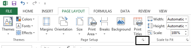
Click Page Layout. Click the small Dialog Box Launcher on the bottom right. This opens up the Page Setup dialog box.

-
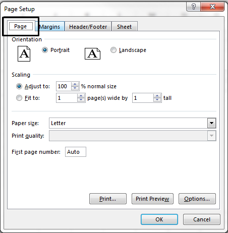
Select the Page tab in the Page Setup dialog box.
-
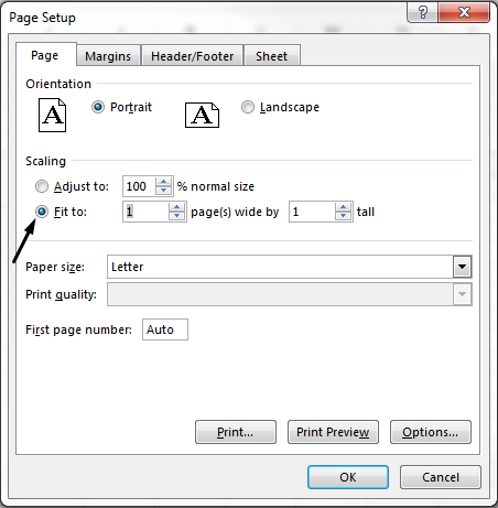
Select Fit to under Scaling.
-
To fit your document to print on one page, choose 1 page(s) wide by 1 tall in the Fit to boxes.
Note: Excel will shrink your data to fit on the number of pages specified. You can also adjust the Fit to numbers to print to multiple pages.
-
Press OK at the bottom of the Page Setup dialog box.
See Also
You can also use page breaks to divide your worksheet into separate pages for printing. While Excel does add page breaks automatically (indicated by a dashed line), you can also insert, move, or delete page breaks in a worksheet.
If you only need to print a section of your worksheet, you can set or clear a print area on a worksheet.
This feature is not available in Excel for the web.
If you have the Excel desktop application, you can use the Open in Excel button to open the workbook and scale the worksheet to fit data on one page.
Page Setup in Excel (Table of Contents)
- Introduction to Page Setup in Excel
- How to Setup Page in Excel?
Introduction to Page Setup in Excel
Often you may come up with a situation where you need to print the excel sheet which you have with yourself, containing some important data that needed to be shared as a hard copy. In such cases, you will be strongly in need of page setup. It becomes easy for you to print the pages once you are well aware of how you can do the same under Microsoft Excel. There are several operations involved under page setup like:
- Setting margins for top, bottom, left and right.
- Adding header or footer to the excel sheet you are going to print.
- Page views: Portrait, landscape or custom.
- Setting printing area etc.
We will go through all the page setup settings and options one by one in this article. It is really very easy under excel to setup the page before printing and previews it to make some amendments as per your need/requirement.
How to Setup Page in Excel?
Page Setup in Excel is very simple and easy. Let’s understand in detail how to setup page in excel.
You can download this Page -Setup- Excel- Template here – Page -Setup- Excel- Template
#1 – Page Setup Using Excel View Tab
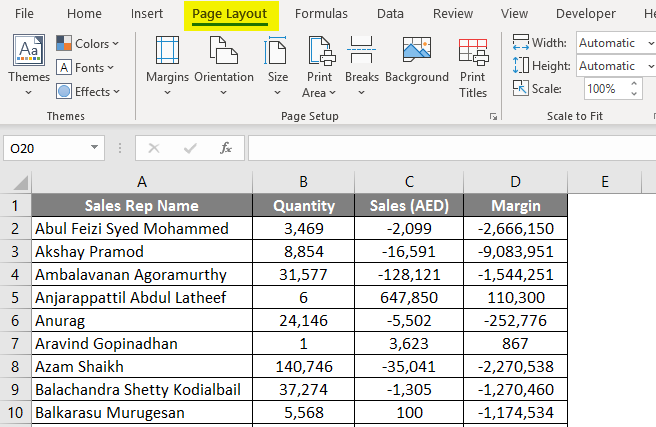
Suppose we have data as shown below:
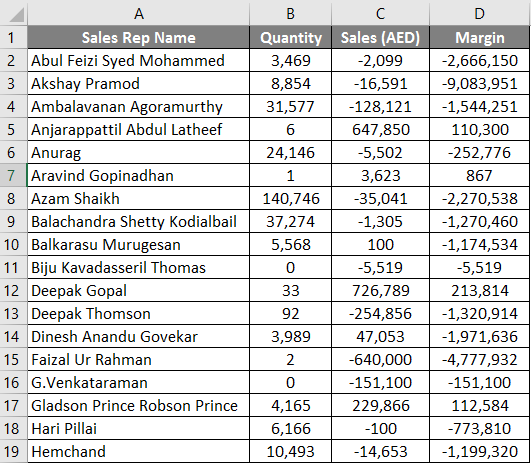
Note: Not all of the data portion is visible in this screenshot.
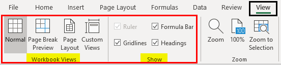
We will see how a basic page setup can be done using Excel’s View tab, present under the top ribbon.
Click on View tab under Excel ribbon which is placed at the top of your sheet. You’ll see multiple operations under two options: “Workbook Views” and “Show”. Under Workbook views, you have different view types: Normal view, Page Break Preview, Page Layout, Custom Views.
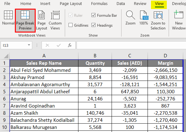
Click on “Page Break Preview”. It will break your page according to the printing area as shown below.
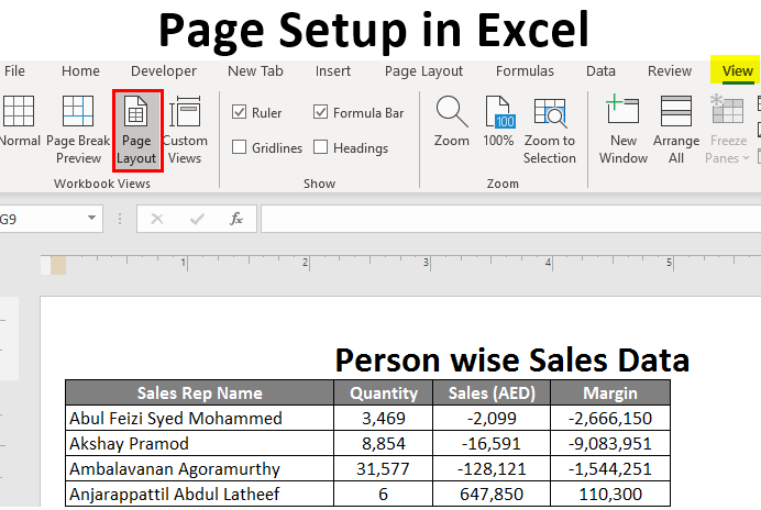
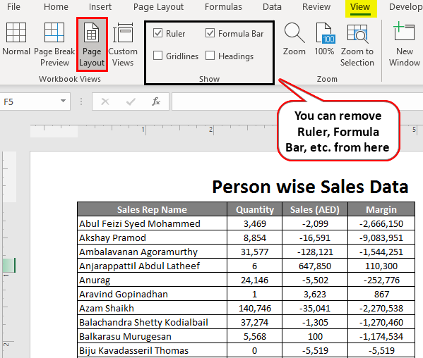
Click on Page Layout option and it will show you the excel sheet in a page layout. It already has Header option by default (I will add ‘Person wise Sales Data’ as a title). Under Show option, you can check or uncheck different options like Ruler, Gridlines, etc.
#2 – Setting up Margins in Excel
We often come up with a situation where the columns from your printing page are occupying the entire page and still have one column, not fitting into the page and it goes to the next printing page for that document. In order to tackle this issue, we can use the margins button/options present under the Page Layout tab in Excel.
Click on the Page Layout tab in excel. You will see a range of operations available each of them consisting of several options.
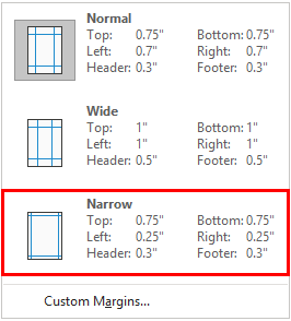
Under “Page Layout”, click on the “Margins” button, you will see different margin options. There are ideally 4 of them: Last Custom Settings, Normal, Wide and Narrow margins. You can select anyone as per your requirement.
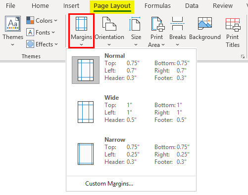
Click on “Narrow” margins, it will narrow down margins and will have more space to acquire the columns.
#3 – Page Orientation under Page Layout
Sometimes, adjusting margin only will not include all your data columns on one page, in that case, you may need to change the page orientation.
Go to “Page Layout” tab and select the Orientation button situated beside the Margins button.
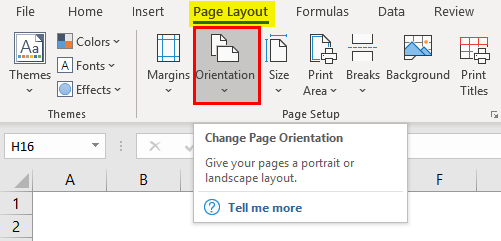
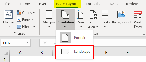
As soon as you click on the Orientation button, you will see two options: Portrait and Landscape.
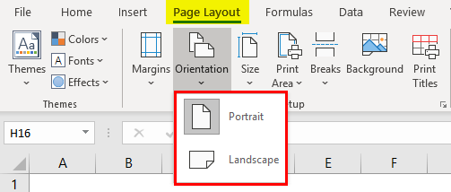
By default, the orientation is in Portrait form. Change it to Landscape so that all your columns can be visible in one single printing page.
Note: Though we are making these amendments/layout settings, data used in this example might not need all those page layout settings. It is just that, we wanted to make you aware of all the page layout settings in one single article.
#4 – Adjusting the Size of Printing Page under Page Layout
You can also change the size of the page in order to get a proper printing page. Go to “Page Layout” tab and click on “Size” button under it. This option allows you to set the paper size for your document when it gets printed.

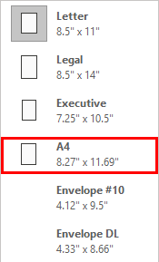
A series of different paper options will appear there. Like Letter, Legal, A4, A3, etc. by default, it will be set to “Letter” page size (As we have changed the orientation to Landscape).
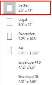
Click on”A4″ to set the page size as A4 (this is the most widely used paper size while printing any document).
#5 – Print Titles Under Page Layout
If your data is long which means it has a large number of rows (say 10,000) it will not fit on one page anyway. It will go on multiple pages. However, the main concern with this is, the column titles are only visible on the first page. What about the next pages where data is populated. It becomes hectic to decide which column is for what. Therefore, having column titles on each page is something which is mandatory while setting page.
Click on “Page Layout” tab and go to “Print Titles” button. Click on that button.
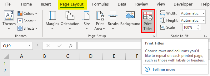
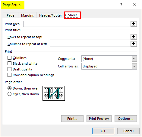
As soon as you click on “Print Titles” button, a new “Page Setup” window will pop up under which “Sheet” option is active (As you have clicked on Print Titles).
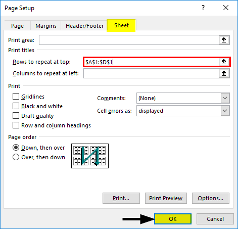
Under it, click on “Rows to repeat at the top option”. This option allows you to add the rows with a title on each page. Once you click on it, you will be in nee q d to select the row ranges which you want to print at the top of every printing page. In our case, it is $A$1:$D$1. Here, in this Sheet option, we also can set the printing area, columns that we want to repeat at the top, etc. Click on OK once done with the amendments.
This is how we setup page before printing in Excel. Let’s wrap the things up with some things to remember.
Things to Remember About Page Setup in Excel
- You can also add custom margins under Page Layout in Excel.
- Print titles and report header, both are different. Print Title prints the title of each column on multiple pages whereas the report header is the header of the report/main title of the report.
- If you want to remove the print titles, go to Page Setup under Print Titles section, select the Sheet tab, and remove the rows provided under Print Titles section.
Recommended Articles
This is a guide to Page Setup in Excel. Here we discuss How to Setup Page in Excel along with practical examples and downloadable excel template. You can also go through our other suggested articles –
- Spelling Check in Excel
- Excel Insert Page Break
- Page Numbers in Excel
- How to Print Labels From Excel
MS-Excel / General Formatting
One of the slickest new features in Excel 2007 is Page Layout View, which shows your worksheet divided up into pages. In
other words, you are able to visualize your printed output as you work. Page Layout View is one of three worksheet views,
which are controlled by the three icons in the right side of the status bar. These views are also available in the View>
Workbook Views group of the Ribbon. The three view options are:
Normal View:
The default view of the worksheet. This view may or may not show page breaks.Page Layout View:
A view that shows individual pages.Page Break Preview:
A view that lets you manually adjust the page breaks.
Just click one of the icons to change the view. You can also use the Zoom slider to change the magnification from 10% (a
very tiny bird’s eye view) to 400% (very large, for showing fine detail). These views can help with printing.
Normal View
Most of the time when you work in Excel, you will use Normal View. Normal View displays page breaks in the worksheet. The
page breaks are indicated by horizontal and vertical dotted lines. These page break lines adjust automatically if you change
the page orientation, add or delete rows or columns, change row heights, change column widths, and so on. For example, if you
find that your printed output is too wide to fit on a single page, you can adjust the column widths (keeping an eye on the page-break
display) until the columns are narrow enough to print on one page.
Page breaks are not displayed until you print (or preview) the worksheet at least one time.
If you’d prefer not to see the page break display in Normal View mode, choose Office> Excel Options and select the Advanced
tab. Scroll down the section titled Display Options For This Worksheet and remove the check mark from Show Page Breaks. This
setting applies only to the active worksheet. Unfortunately, the option to turn off page break display is not in the Ribbon,
and it’s not even available for inclusion on the Quick Access Toolbar.
A worksheet in Normal View mode, zoomed out to show multiple pages. Notice the dotted lines that indicate page breaks.
Page Layout View
Page Layout View is the ultimate print preview. Unlike the old print preview, this mode is not a view only mode. You have
complete access to all Excel commands. In fact, you can use Page Layout View all the time if you like.
A worksheet in Page Layout View, zoomed out to show multiple pages. Notice that The page header & footer (if any) appear
on each page, giving you a true preview of the printed output.
If you move the mouse to the corner of a page while in Page Layout View, you can click to hide the white space in the margins.
Doing so gives you all the advantages of Page Layout View, but you can see more information on screen because the unused margin space is hidden.
In Page Layout View, the worksheet resembles printed pages.
Page Break Preview
Page Break Preview displays the worksheet and shows where the page breaks occur. This view mode is different from Normal
View mode with page breaks turned on. The key difference is that you can drag the page breaks. Unlike Page Layout View, Page
Break Preview does not display headers and footers.
When you enter Page Break Preview mode, Excel performs the following:
- Changes the zoom factor so that you can see more of the worksheet.
- Displays the page numbers overlaid on the pages.
- Displays the current print range with a white background; nonprinting data appears with a gray background.
- Displays all page breaks as draggable dashed lines.
When you change the page breaks by dragging, Excel automatically adjusts the scaling so that the information fits on the
pages, per your specifications.
In Page Break Preview mode, you still have access to all of Excel’s commands. You can change the zoom factor if you find
the text to be too small.
To exit Page Break Preview mode, just click one of the other View icons in the status bar.

How to Set up Page in Excel? (5 Easy Steps)
To make the page come on a single page, we need to set up the page. First, we must follow the steps below to set up the page in Excel.
Table of contents
- How to Set up Page in Excel? (5 Easy Steps)
- How to Change the Default Page Setup in Excel?
- Step #1 – Setup Print Area
- Step #2 – Page Break View
- Print Rows and Column Headings Along with the Data
- Print Data Headers in all the Pages
- Things to Remember Here
- Recommended Articles
- How to Change the Default Page Setup in Excel?
To set up the page, follow the below steps in Excel.
- First, go to the “Page Layout” tab and click on the small arrow mark under the “Page Setup” group.

- Once you click on a small arrow mark, it will open up the below dialog box.

- In the below window, in”Fit to:” write 1 page.

- Click on “Print Preview” in the same window to see the same preview.
- Now, we can see the print preview.


It looks on one page but is not able to read properly. Change the orientation from “Portrait” to “Landscape” in the same print preview window.

Now, our print preview looks like this.

How to Change the Default Page Setup in Excel?
Below are the steps to change the default page setup in Excel.
Step #1 – Setup Print Area
The first thing we need to do while printing is to set the print area. For example, look at the below data in a worksheet.

First, select the print areaIn Excel, the print area is the portion of the workbook or worksheet that we wish to be printed rather than the entire workbook or worksheet. From the page out tab, we can set up a print area. In addition, a single worksheet can contain numerous print areas.read more; data range from A1:N32. After selecting the data range, go to PAGE LAYOUT >>> Print Area >>> Set Print Area.

It will set up the print area.
The shortcut key to set up the print area is ALT + P + R + S.

Step #2 – Page Break View
Once the print area is set up, we cannot simply print the data because the data is not in order. For example, we must press Ctrl + P to see the Print previewPrint preview in Excel is a tool used to represent the print output of the current page in the excel to see if any adjustments need to be made in the final production. Print preview only displays the document on the screen, and it does not print.read more.

As we can see in the above image, data is not coming in order from column A to column L. Instead, it is coming on one page, and the remaining portion is coming on other pages.
So, if we print like this, we cannot read the report properly.
To check which data is coming in the first sheet and which is coming in the second sheet, go to the VIEW tab and click on “Page Break Preview.”


In the above image, we can see the “Page Break Preview.” The blue line (next to column L) is the indication that column A to column L belongs to Page 1.
The remaining columns, M and N, will come in the next pages.
Print Rows and Column Headings Along with the Data
Not only can we print the data, but we can also print excel rows and columnsA cell is the intersection of rows and columns. Rows and columns make the software that is called excel. The area of excel worksheet is divided into rows and columns and at any point in time, if we want to refer a particular location of this area, we need to refer a cell.read more headings. Numbers represent row headings, and alphabets represent column headings.

We need to make some settings for printing these rows and column headers along with the data.
Go to the “PAGE LAYOUT” tab and click on the small arrow mark under the “Page Setup” group in ExcelThe “Group” is an Excel tool which groups two or more rows or columns. With grouping, the user has an option to minimize and maximize the grouped data.read more.

Once you click on the small arrow mark, it will open up the below dialog box.

In the above window, click on the “Sheet” tab. Under this tab, we have several options. First, check the “Row and column headings” box, then click on “Print Preview” to see the view.

As shown in the below image, we can see row and column headings.

Once the data is extended to multiple sheets, we do not get data headers on all the pages. It makes the report reading very difficult. So, in these numerous printing sheets, we need to change the settings to “Repeat the rows.”
In the “Page Setup” Excel window, go to the “Sheet” tab. This tab has an option called “Rows to repeat at top.”

In this option, a cursor inside the box chooses the data header row to repeat the headers in all the print pages. Click on “OK.” It will repeat the row at the top in all the sheets.

Things to Remember Here
- We must first set up the print area.
- It depends on the data size. But, first, we need to choose an orientation style.
- We can repeat excel row headersExcel Row Header is the grey column on the left side of column 1 in the worksheet that contains the numbers (1, 2, 3, etc.). To hide or reveal row and column headers, press ALT + W + V + H.read more and column headers.
- We can also repeat data headers in all the printing sheets.
Recommended Articles
This article is a guide to Page Setup in Excel. We discuss using page setup in Excel, practical examples, and downloadable templates. You may also learn more about Excel from the following articles: –
- Print Preview in Excel
- Insert Page Break in Excel
- Print Titles in Excel
- Print Excel Gridlines
- Excel Shortcut for Merge and Center