
The SpecialCells Does not actually work as it needs to be continuous. I have solved this by adding a sort funtion in order to sort the data based on the coloumns i need.
Sorry for no comments on the code as i was not planning to share it:
Sub testtt()
    arr = FilterAndGetData(Worksheets("Data").range("A:K"), Array(1, 9), Array("george", "WeeklyCash"), Array(1, 2, 3, 10, 11), 1)
    Debug.Print sms(arr)
End Sub
Function FilterAndGetData(ByVal rng As Variant, ByVal fields As Variant, ByVal criterias As Variant, ByVal colstoreturn As Variant, ByVal headers As Boolean) As Variant
Dim SUset, EAset, CMset
If Application.ScreenUpdating Then Application.ScreenUpdating = False: SUset = False Else SUset = True
If Application.EnableEvents Then Application.EnableEvents = False: EAset = False Else EAset = True
If Application.Calculation = xlCalculationAutomatic Then Application.Calculation = xlCalculationManual: CMset = False Else CMset = True
For Each col In rng.Columns: col.Hidden = False: Next col

Dim oldsheet, scol, ecol, srow, hyesno As String
Dim i, counter As Integer

oldsheet = ActiveSheet.Name


Worksheets(rng.Worksheet.Name).Activate

Worksheets(rng.Worksheet.Name).AutoFilterMode = False

scol = Chr(rng.Column + 64)
ecol = Chr(rng.Columns.Count + rng.Column + 64 - 1)
srow = rng.row

If UBound(fields) - LBound(fields) <> UBound(criterias) - LBound(criterias) Then FilterAndGetData = "Fields&Crit. counts dont match": GoTo done

dd = sortrange(rng, colstoreturn, headers)

For i = LBound(fields) To UBound(fields)
    rng.AutoFilter Field:=CStr(fields(i)), Criteria1:=CStr(criterias(i))
Next i

Dim rngg As Variant

rngg = rng.SpecialCells(xlCellTypeVisible)
Debug.Print ActiveSheet.AutoFilter.range.address
FilterAndGetData = ActiveSheet.AutoFilter.range.SpecialCells(xlCellTypeVisible).Value

For Each row In rng.Rows
    If row.EntireRow.Hidden Then Debug.Print yes
Next row


done:
    'Worksheets("Data").AutoFilterMode = False
    Worksheets(oldsheet).Activate
    If SUset Then Application.ScreenUpdating = True
    If EAset Then Application.EnableEvents = True
    If CMset Then Application.Calculation = xlCalculationAutomatic
End Function
Function sortrange(ByVal rng As Variant, ByVal colnumbers As Variant, ByVal headers As Boolean)

    Dim SUset, EAset, CMset
    If Application.ScreenUpdating Then Application.ScreenUpdating = False: SUset = False Else SUset = True
    If Application.EnableEvents Then Application.EnableEvents = False: EAset = False Else EAset = True
    If Application.Calculation = xlCalculationAutomatic Then Application.Calculation = xlCalculationManual: CMset = False Else CMset = True
    For Each col In rng.Columns: col.Hidden = False: Next col

    Dim oldsheet, scol, srow, sortcol, hyesno As String
    Dim i, counter As Integer
    oldsheet = ActiveSheet.Name
    Worksheets(rng.Worksheet.Name).Activate
    Worksheets(rng.Worksheet.Name).AutoFilterMode = False
    scol = rng.Column
    srow = rng.row

    If headers Then hyesno = xlYes Else hyesno = xlNo

    For i = LBound(colnumbers) To UBound(colnumbers)
        rng.Sort key1:=range(Chr(scol + colnumbers(i) + 63) + CStr(srow)), order1:=xlAscending, Header:=hyesno
    Next i
    sortrange = "123"
done:
    Worksheets(oldsheet).Activate
    If SUset Then Application.ScreenUpdating = True
    If EAset Then Application.EnableEvents = True
    If CMset Then Application.Calculation = xlCalculationAutomatic
End Function
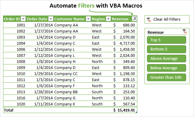
Bottom line: Learn how to create macros that apply filters to ranges and Tables with the AutoFilter method in VBA. The post contains links to examples for filtering different data types including text, numbers, dates, colors, and icons.
Skill level: Intermediate
Download the File
The Excel file that contains the code can be downloaded below. This file contains code for filtering different data types and filter types.
Writing Macros for Filters in Excel
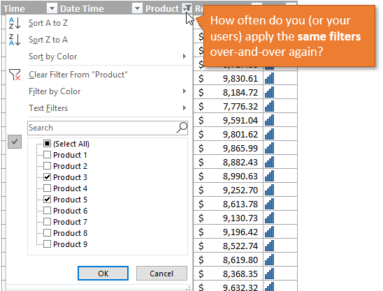
Filters are a great tool for analyzing data in Excel. For most analysts and frequent Excel users, filters are a part of our daily lives. We use the filter drop-down menus to apply filters to individual columns in a data set. This helps us tie out numbers with reports and do investigative work on our data.
Filtering can also be a time consuming process. Especially when we are applying filters to multiple columns on large worksheets, or filtering data to then copy/paste it to other worksheets or workbooks.
This article explains how to create macros to automate the filtering process. This is an extensive guide on the AutoFilter method in VBA.
I also have articles with examples for different filters and data types including: blanks, text, numbers, dates, colors & icons, and clearing filters.
The Macro Recorder is Your Friend (& Enemy)
We can easily get the VBA code for filters by turning on the macro recorder, then applying one or more filters to a range/Table.
Here are the steps to create a filter macro with the macro recorder:
- Turn the macro recorder on:
- Developer tab > Record Macro.
- Give the macro a name, choose where you want the code saved, and press OK.
- Apply one or more filters using the filter drop-down menus.
- Stop the recorder.
- Open the VB Editor (Developer tab > Visual Basic) to view the code.
If you’ve already used the macro recorder for this process, then you know how useful it can be. Especially as our filter criteria gets more complex.
The code will look something like the following.
Sub Filters_Macro_Recorder()
'
' Filters_Macro_Recorder Macro
'

'
    ActiveSheet.ListObjects("tblData").Range.AutoFilter Field:=4, Criteria1:= _
        "Product 2"
    ActiveSheet.ListObjects("tblData").Range.AutoFilter Field:=4
    ActiveSheet.ListObjects("tblData").Range.AutoFilter Field:=5, Criteria1:= _
        ">=500", Operator:=xlAnd, Criteria2:="<=1000"
End Sub
We can see that each line uses the AutoFilter method to apply the filter to the column. It also contains information about the criteria for the filter.
This is where it can get complex, confusing, and frustrating. It can be difficult to understand what the code means when trying to modify it for a different data set or scenario. So let’s take a look at how the AutoFilter method works.
The AutoFilter Method Explained
The AutoFilter method is used to clear and apply filters to a single column in a range or Table in VBA. It automates the process of applying filters through the filter drop-down menus, and does all that work for us. 🙂
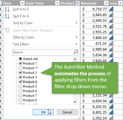
It can be used to apply filters to multiple columns by writing multiple lines of code, one for each column. We can also use AutoFilter to apply multiple filter criteria to a single column, just like you would in the filter drop-down menu by selecting multiple check boxes or specifying a date range.
Writing AutoFilter Code
Here are step-by-step instructions for writing a line of code for AutoFilter
Step 1 : Referencing the Range or Table
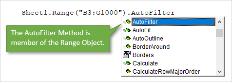
The AutoFilter method is a member of the Range object. So we must reference a range or Table that the filters are applied to on the sheet. This will be the entire range that the filters are applied to.
The following examples will enable/disable filters on range B3:G1000 on the AutoFilter Guide sheet.
Sub AutoFilter_Range()
'AutoFilter is a member of the Range object

  'Reference the entire range that the filters are applied to
  'AutoFilter turns filters on/off when no parameters are specified.
  Sheet1.Range("B3:G1000").AutoFilter

  'Fully qualified reference starting at Workbook level
  ThisWorkbook.Worksheets("AutoFilter Guide").Range("B3:G1000").AutoFilter

End Sub
Here is an example using Excel Tables.
Sub AutoFilter_Table()
'AutoFilters on Tables work the same way.

Dim lo As ListObject 'Excel Table

  'Set the ListObject (Table) variable
  Set lo = Sheet1.ListObjects(1)

  'AutoFilter is member of Range object
  'The parent of the Range object is the List Object
  lo.Range.AutoFilter

End Sub
The AutoFilter method has 5 optional parameters, which we’ll look at next. If we don’t specify any of the parameters, like the examples above, then the AutoFilter method will turn the filters on/off for the referenced range. It is toggle. If the filters are on they will be turned off, and vice-versa.
Ranges or Tables?
Filters work the same on both regular ranges and Excel Tables.
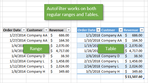
My preferred method is to use Tables because we don’t have to worry about changing range references as the table grows or shrinks. However, the code will be the same for both objects. The rest of the code examples use Excel tables, but you can easily modify this for regular ranges.
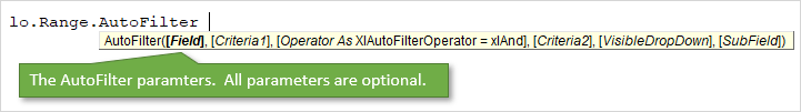
The 5 (or 6) AutoFilter Paramaters
The AutoFilter method has 5 (or 6) optional parameters that are used to specify the filter criteria for a column. Here is a list of the parameters.
| Name | Req/Opt | Description |
|---|---|---|
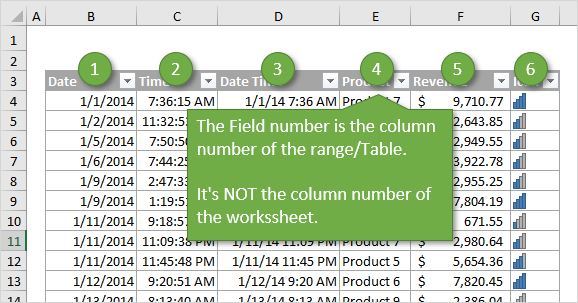
| Field | Optional | The number of the column within the filter range that the filter will be applied to. This is the column number within the filter range, NOT the column number of the worksheet. |
| Criteria1 | Optional | A string wrapped in quotation marks that is used to specify the filter criteria. Comparison operators can be included for less than or greater than filters. Many rules apply depending on the data type of the column. See examples below. |
| Operator | Optional | Specifies the type of filter for different data types and criteria by using one of the XlAutoFilterOperator constants. See this MSDN help page for a detailed list, and list in macro examples below. |
| Criteria2 | Optional | Used in combination with the Operator parameter and Criteria1 to create filters for multiple criteria or ranges. Also used for specific date filters for multiple items. |
| VisibleDropDown | Optional | Displays or hides the filter drop-down button for an individual column (field). |
| Subfield | Optional | Not sure yet… |
We can use a combination of these parameters to apply various filter criteria for different data types. The first four are the most important, so let’s take a look at how to apply those.
Step 2: The Field Parameter
The first parameter is the Field. For the Field parameter we specify a number that is the column number that the filter will be applied to. This is the column number within the filter range that is the parent of the AutoFilter method. It is NOT number of the column on the worksheet.
In the example below Field 4 is the Product column because it is the 4th column in the filter range/Table.
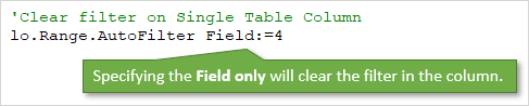
The column filter is cleared when we only specify the the Field parameter, and no other criteria.
We can also use a variable for the Field parameter and set it dynamically. I explain that in more detail below.
Step 3: The Criteria Parameters
There are two parameters that can be used to specify the filter Criteria, Criteria1 and Criteria2. We use a combination of these parameters and the Operator parameter for different types of filters. This is where things get tricky, so let’s start with a simple example.
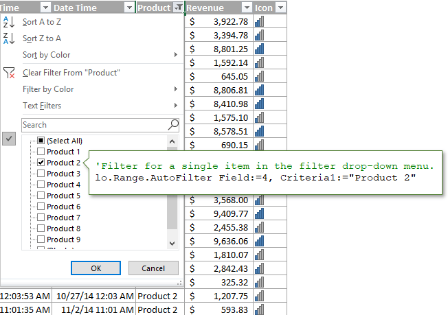
'Filter the Product column for a single item
lo.Range.AutoFilter Field:=4, Criteria1:="Product 2"
This would be the same as selecting a single item from the checkbox list in the filter drop-down menu.
General Rules for Criteria1 and Criteria2
The values we specify for Criteria1 and Criteria2 can get tricky. Here are some general guidelines for how to reference the Criteria parameter values.
- The criteria value is a string wrapped in quotation marks. There are a few exceptions where the criteria is a constant for date time period and above/below average.
- When specifying filters for single numbers or dates, the number formatting must match the number formatting that is applied in the range/table.
- The comparison operator for greater/less than is also included inside the quotation marks, before the number.
- Quotation marks are also used for filters for blanks “=” and non-blanks “<>”.
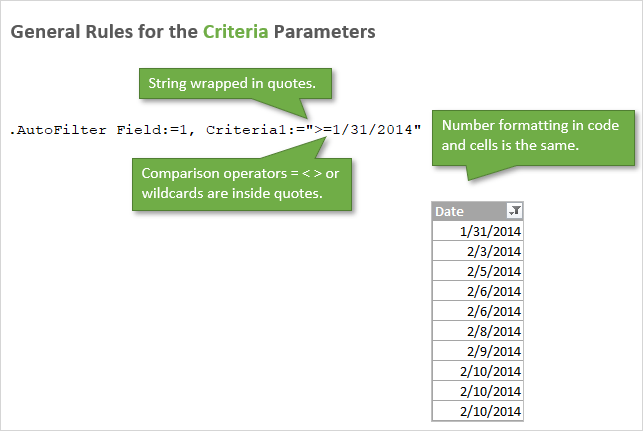
'Filter for date greater than or equal to Jan 1 2015
lo.Range.AutoFilter Field:=1, Criteria1:=">=1/1/2015"

' The comparison operator >= is inside the quotation marks
' for the Criteria1 parameter.

' The date formatting in the code matches the formatting
' applied to the cells in the worksheet.
Step 4: The Operator Parameter
What if we want to select multiple items from the filter drop-down? Or do a filter for a range of dates or numbers?
For this we need the Operator. The Operator parameter is used to specify what type of filter we want to apply. This can vary based on the type of data in the column. One of the following 11 constants must be used for the Operator.
| Name | Value | Description |
|---|---|---|
| xlAnd | 1 | Include both Criteria1 and Criteria2. Can be used for date or number ranges. |
| xlBottom10Items | 4 | Lowest-valued items displayed (number of items specified in Criteria1). |
| xlBottom10Percent | 6 | Lowest-valued items displayed (percentage specified in Criteria1). |
| xlFilterCellColor | 8 | Fill Color of the cell |
| xlFilterDynamic | 11 | Dynamic filter used for Above/Below Average and Date Periods |
| xlFilterFontColor | 9 | Color of the font in the cell |
| xlFilterIcon | 10 | Filter icon created by conditional formatting |
| xlFilterValues | 7 | Used for filters with multiple criteria specified with an Array function. |
| xlOr | 2 | Include either Criteria1 or Criteria2. Can be used for date and number ranges. |
| xlTop10Items | 3 | Highest-valued items displayed (number of items specified in Criteria1). |
| xlTop10Percent | 5 | Highest-valued items displayed (percentage specified in Criteria1). |
Here is a link to the MSDN help page that contains the list of constants for XlAutoFilterOperator Enumeration.
The operator is used in combination with Criteria1 and/or Criteria2, depending on the data type and filter type. Here are a few examples.
'Filter for list of multiple items, Operator is xlFilterValues
lo.Range.AutoFilter _
          Field:=iCol, _
          Criteria1:=Array("Product 4", "Product 5", "Product 6"), _
          Operator:=xlFilterValues
'Filter for Date Range (between dates), Operator is xlAnd
lo.Range.AutoFilter _
          Field:=iCol, _
          Criteria1:=">=1/1/2014", _
          Operator:=xlAnd, _
          Criteria2:="<=12/31/2015"
So that is the basics of writing a line of code for the AutoFilter method. It gets more complex with different data types. So I’ve provided many examples below that contain most of the combinations of Criteria and Operator for different types of filters.
AutoFilter is NOT Additive
When an AutoFilter line of code is run, it first clears any filters applied to that column (Field), then applies the filter criteria that is specified in the line of code.
This means it is NOT additive. The following 2 lines will NOT create a filter for Product 1 and Product 2. After the macro is run, the Product column will only be filtered for Product 2.
'AutoFilter is NOT addititive.  It first any filters applied
'in the column before applying the new filter
lo.Range.AutoFilter Field:=4, Criteria1:="Product 3"

'This line of code will filter the column for Product 2 only
'The filter for Product 3 above will be cleared when this line runs.
lo.Range.AutoFilter Field:=4, Criteria1:="Product 2"
If you want to apply a filter with multiple criteria to a single column, then you can specify that with the Criteria and Operator parameters.
How to Set the Field Number Dynamically
If we add/delete/move columns in the filter range, then the field number for a filtered column might change. Therefore, I try to avoid hard-coding a number for the Field parameter whenever possible.
We can use a variable instead and use some code to find the column number by it’s name. Here are two examples for regular ranges and Tables.
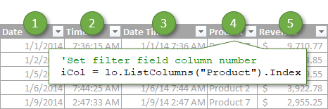
Sub Dynamic_Field_Number()
'Techniques to find and set the Field based on the column name.

Dim lo As ListObject
Dim iCol As Long

  'Set reference to the first Table on the sheet
  Set lo = Sheet1.ListObjects(1)

  'Set filter field
  iCol = lo.ListColumns("Product").Index

  'Use Match function for regular ranges
  'iCol = WorksheetFunction.Match("Product", Sheet1.Range("B3:G3"), 0)

  'Use the variable for the Field parameter value
  lo.Range.AutoFilter Field:=iCol, Criteria1:="Product 3"

End Sub
The column number will be found every time we run the macro. We don’t have to worry about changing the field number when the column moves. This saves time and prevents errors (win-win)! 🙂
Use Excel Tables with Filters
There are a lot of advantages to using Excel Tables, especially with the AutoFilter method. Here are a few of the major reasons I prefer Tables.
- We don’t have to redefine the range in VBA as the data range changes size (rows/columns are added/deleted). The entire Table is referenced with the ListObject object.
- It’s easy to reference the data in the Table after filters are applied. We can use the DataBodyRange property to reference visible rows to copy/paste, format, modify values, etc.
- We can have multiple Tables on the same sheet, and therefore multiple filter ranges. With regular ranges we can only have one filtered range per sheet.
- The code to clear all filters on a Table is easier to write.
Filters & Data Types
The filter drop-down menu options change based on what type of data is in the column. We have different filters for text, numbers, dates, and colors. This creates A LOT of different combinations of Operators and Criteria for each type of filter.
I created separate posts for each of these filter types. The posts contain explanations and VBA code examples.
- How to Clear Filters with VBA
- How to Filter for Blank & Non-Blank Cells
- How to Filter for Text with VBA
- How to Filter for Numbers with VBA
- How to Filter for Dates with VBA
- How to Filter for Colors & Icons with VBA
The file in the downloads section above contains all of these code samples in one place. You can add it to your Personal Macro Workbook and use the macros in your projects.
Why is the AutoFilter Method so Complex?
This post was inspired by a question from Chris, a member of The VBA Pro Course. The combinations of Criteria and Operators can be confusing and complex. Why is this?
Well, filters have evolved over the years. We saw a lot of new filter types introduced in Excel 2010, and the feature is continuing to be improved. However, the parameters of the AutoFilter method haven’t changed. This is great for compatibility with older versions, but also means the new filter types are being worked into the existing parameters.
Most of the filter code makes sense, but can be tricky to figure out at first. Fortunately we have the macro recorder to help with that.
I hope you can use this post and Excel file as a guide to writing macros for filters. Automating filters can save us and our users a ton of time, especially when using these techniques in a larger data automation project.
Please leave a comment below with any questions or suggestions. Thank you! 🙂
Стандартный Автофильтр для выборки из списков — вещь, безусловно, привычная и надежная. Но для создания сложных условий приходится выполнить не так уж мало действий. Например, чтобы отфильтровать значения попадающие в интервал от 100 до 200, необходимо развернуть список Автофильтра мышью, выбрать вариант Условие (Custom), а в новых версиях Excel: Числовые фильтры — Настраиваемый фильтр (Number filters — Custom filter). Затем в диалоговом окне задать два оператора сравнения, значения и логическую связку (И-ИЛИ) между ними:

Не так уж и долго, скажут некоторые. Да, но если в день приходится повторять эту процедуру по нескольку десятков раз? Выход есть — альтернативный фильтр с помощью макроса, который будет брать значения критериев отбора прямо из ячеек листа, куда мы их просто введем с клавиатуры. По сути, это будет похоже на расширенный фильтр, но работающий в реальном времени. Чтобы реализовать такую штуку, нам потребуется сделать всего два шага:
Шаг 1. Именованный диапазон для условий
Сначала надо создать именованный диапазон, куда мы будем вводить условия, и откуда макрос их будет брать. Для этого можно прямо над таблицей вставить пару-тройку пустых строк, затем выделить ячейки для будущих критериев (на рисунке это A2:F2) и дать им имя Условия, вписав его в поле имени в левом верхнем углу и нажав клавишу Enter. Для наглядности, я выделил эти ячейки желтым цветом:

Шаг 2. Добавляем макрос фильтрации
Теперь надо добавить к текущему листу макрос фильтрации по критериям из созданного диапазона Условия. Для этого щелкните правой кнопкой мыши по ярлычку листа и выберите команду Исходный текст (Source text). В открывшееся окно редактора Visual Basic надо скопировать и вставить текст вот такого макроса:
Private Sub Worksheet_Change(ByVal Target As Range)

    Dim FilterCol As Integer
    Dim FilterRange As Range
    Dim CondtitionString As Variant
    Dim Condition1 As String, Condition2 As String

    If Intersect(Target, Range("Условия")) Is Nothing Then Exit Sub

    On Error Resume Next
    Application.ScreenUpdating = False

    'определяем диапазон данных списка
    Set FilterRange = Target.Parent.AutoFilter.Range

    'считываем условия из всех измененных ячеек диапазона условий
    For Each cell In Target.Cells
        FilterCol = cell.Column - FilterRange.Columns(1).Column + 1

        If IsEmpty(cell) Then
            Target.Parent.Range(FilterRange.Address).AutoFilter Field:=FilterCol
        Else
            If InStr(1, UCase(cell.Value), " ИЛИ ") > 0 Then
                LogicOperator = xlOr
                ConditionArray = Split(UCase(cell.Value), " ИЛИ ")
            Else
                If InStr(1, UCase(cell.Value), " И ") > 0 Then
                    LogicOperator = xlAnd
                    ConditionArray = Split(UCase(cell.Value), " И ")
                Else
                    ConditionArray = Array(cell.Text)
                End If
            End If
            'формируем первое условие
            If Left(ConditionArray(0), 1) = "<" Or Left(ConditionArray(0), 1) = ">" Then
                Condition1 = ConditionArray(0)
            Else
                Condition1 = "=" & ConditionArray(0)
            End If
            'формируем второе условие - если оно есть
            If UBound(ConditionArray) = 1 Then
                If Left(ConditionArray(1), 1) = "<" Or Left(ConditionArray(1), 1) = ">" Then
                    Condition2 = ConditionArray(1)
                Else
                    Condition2 = "=" & ConditionArray(1)
                End If
            End If
            'включаем фильтрацию
            If UBound(ConditionArray) = 0 Then
                Target.Parent.Range(FilterRange.Address).AutoFilter Field:=FilterCol, Criteria1:=Condition1
            Else
                Target.Parent.Range(FilterRange.Address).AutoFilter Field:=FilterCol, Criteria1:=Condition1, _
                    Operator:=LogicOperator, Criteria2:=Condition2
            End If
        End If
    Next cell

    Set FilterRange = Nothing
    Application.ScreenUpdating = True
End Sub
Все.
Теперь при вводе любых условий в желтые ячейки нашего именованного диапазона тут же будет срабатывать фильтрация, отображая только нужные нам строки и скрывая ненужные:

Как и в случае с классическими Автофильтром (Filter) и Расширенным фильтром (Advanced Filter), в нашем фильтре макросом можно смело использовать символы подстановки:
- * (звездочка) — заменяет любое количество любых символов
- ? (вопросительный знак) — заменяет один любой символ
и операторы логической связки:
- И — выполнение обоих условий
- ИЛИ — выполнение хотя бы одного из двух условий
и любые математические символы неравенства (>,<,=,>=,<=,<>).
При удалении содержимого ячеек желтого диапазона Условия автоматически снимается фильтрация с соответствующих столбцов.
P.S.
- Если у вас Excel 2007 или 2010 не забудьте сохранить файл с поддержкой макросов (в формате xlsm), иначе добавленный макрос умрет.
- Данный макрос не умеет работать с «умными таблицами»
Ссылки по теме
- Что такое макросы, куда вставлять код макроса на VBA, как их использовать?
- Умные таблицы Excel 2007/2010
- Расширенный фильтр и немного магии
Excel VBA Filter
VBA Filter tool one can use to sort out or fetch the specific data desired. For example, one can use the Autofilter function as a worksheet function. However, this function has other arguments with it which are optional, and the only mandatory argument is the expression that covers the range. For example, worksheets(“Sheet1”).Range(“A1”).Autofilter will apply the filter on the first column.
Filter in VBA works the same way it works in the worksheet. The only thing different is we can automate the routine task of filtering the data through coding.
Table of contents
- Excel VBA Filter
- Examples to Filter Data using VBA
- Example #1 – Apply or Remove Filter to the Data
- Step 1: Supply data range
- Step 2: Then access AutoFilter function
- Step 3: Run the code to enable the filter
- Example #2 – Filter Specific Values
- Step 1: Select Range and Open Autofilter Function
- Step 2: Then Select Field
- Step 3: Now Mention Criteria
- Step 4: And run the code
- Example #3 – Usage of OPERATOR Argument
- Step 1: Select Range and Autofilter Field
- Step 2: Enter Criteria 1 as Math
- Step 3: Use Operator xl
- Step 4: Enter Criteria 2 as Politics
- Example #4 – Filter Numbers with Operator Symbols
- Example #5 – Apply Filter for More Than One Column
- Example #1 – Apply or Remove Filter to the Data
- Things to Remember
- Recommended Articles
- Examples to Filter Data using VBA
You are free to use this image on your website, templates, etc, Please provide us with an attribution linkArticle Link to be Hyperlinked
For eg:
Source: VBA Filter Data (wallstreetmojo.com)
The AutoFilter is a function that includes many syntax values. Below are the parameters involved in the AutoFilter function.
![]()
- The range is the first thing we need to supply to use the “AutoFilter” option. After that, it is simply for which range of cells we need to apply the filter, for example, Range (“A1:D50”).
- The field is the first argument in the function. Once we select the range of cells through the VBA RANGE objectRange is a property in VBA that helps specify a particular cell, a range of cells, a row, a column, or a three-dimensional range. In the context of the Excel worksheet, the VBA range object includes a single cell or multiple cells spread across various rows and columns.read more, we need to mention for which column of the range we want to apply the filter for.
- Criteria 1 is nothing, but in the selected Field, the value that you want to filter out.
- The operator we may use if we want to use the Criteria 2 argument. In this option, we can use the below options.
xlAnd, xlOr, xlBottom10Items, xlTop10Items, xlTop10Percent, xlBottom10Percent, xlFilterCellColor, xlFilterDynamic, xlFilterFontColor, xlFilterIcon, xlFilterValues - Visible Dropdown displays a filter symbol in the filter applied column. If you want to display it, you can supply the argument as TRUE or else FALSE.
Examples to Filter Data using VBA
You can download this VBA Filter Excel Template here – VBA Filter Excel Template
Example #1 – Apply or Remove Filter to the Data
If you want to apply the filter option to the data, then we can turn it off and on this option. For example, look at the below data image.
Step 1: Supply data range
To activate the filter option first, we need to supply what is our data range. For example, in the above image, our data is spread from A1 to G31. So, supply this range using a RANGE object.
Code:
Sub Filter_Example()

  Range ("A1:G31")

End Sub

Step 2: Then access AutoFilter function
Now, access the AutoFilter function for this range.
Code:
Sub Filter_Example()

  Range("A1:G31").AutoFilter

End Sub

Step 3: Run the code to enable the filter
That is all. Run this code to enable the AutoFilter.

This code works as a toggle. If the filter is not applied, it will apply. If already applied, then it will be removed.
Example #2 – Filter Specific Values
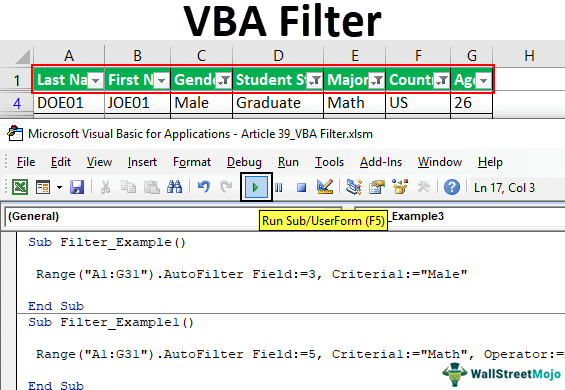
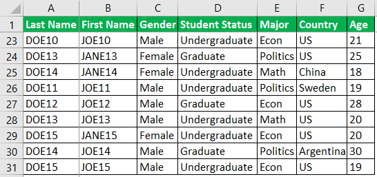
Now, we will see how to use the parameters of the AutoFilter option. Take the same data as above. For example, we must filter out all “Male” gender names.
Step 1: Select Range and Open Autofilter Function

Step 2: Then Select Field
In the function’s first argument, i.e., Field, we need to mention the column reference we would like to filter out. In this example, we need to filter only “Male” candidates, column “C,” so the column number is 3.

Step 3: Now Mention Criteria
Now for this supplied Field, we need to mention Criteria 1, i.e., what value we need to filter in the Field. We need to filter “Male” from this column.
Code:
Sub Filter_Example()

  Range("A1:G31").AutoFilter Field:=3, Criteria1:="Male"

End Sub

Step 4: And run the code
Ok, that’s all. So this code will filter only “Male” candidates now.

Example #3 – Usage of OPERATOR Argument
When you want to filter out more than one value from the column, we need to use the “Operator” argument. For example, from the column “Major,” we need to filter only “Math & Politics,” then we need to use this argument.
Step 1: Select Range and Autofilter Field
First, supply the Range of cells and fields.
Code:
Sub Filter_Example()

 Range("A1:G31").AutoFilter Field:=5,

End Sub

Step 2: Enter Criteria 1 as Math
For the mentioned field, we need to supply Criteria 1 as “Math.”
Code:
Sub Filter_Example()

 Range("A1:G31").AutoFilter Field:=5, Criteria1:="Math",

End Sub

Step 3: Use Operator xl
Since we need to filter one more value from the same column or field, use the operator symbol as “xlOr.”
Code:
Sub Filter_Example()

  Range("A1:G31").AutoFilter Field:=5, Criteria1:="Math",
  Operator:=xlOr

End Sub

Step 4: Enter Criteria 2 as Politics
And for Criteria 2 argument, mention the value as “Politics.”
Code:
Sub Filter_Example()

 Range("A1:G31").AutoFilter Field:=5, Criteria1:="Math",
 Operator:=xlOr, Criteria2:="Politics"

End Sub

It will filter out both “Math” and “Politics” from column “Major.”

Example #4 – Filter Numbers with Operator Symbols
For example, if you want to filter numbers, we can filter a specific number and numbers above, below, or between specific values and a range of values.
For example, if you want to filter persons aged more than 30, then we can write the code below from the age column.
Code:
Sub Filter_Example()

 Range("A1:G31").AutoFilter Field:=7, Criteria1:=">30"

End Sub
It will filter all the values that are more than 30.
Now, if you want to filter values between 21 and 31, we can use the code below.
Code:
Sub Filter_Example()

 Range("A1:G31").AutoFilter Field:=7, Criteria1:=">21",
 Operator:=xlAnd, Criteria2:="<31"

End Sub
It will filter persons aged between 21 and 30.
Example #5 – Apply Filter for More Than One Column
We need to use a slightly different technique if you want to filter values from more than one column criteria.
If you want to filter “Student Status” as “Graduate” and “Country” as “US,” then first, we need to supply the RANGE of cells under the WITH statement.
Code:
Sub Filter_Example()

  With Range("A1:G31")

  End With

End Sub

Inside the WITH statement, supply the first criteria to be filtered.
Code:
Sub Filter_Example()

 With Range("A1:G31")
  .AutoFilter Field:=4, Criteria1:="Graduate"
 End With

End Sub

Now, in the next line, do the same for “Country” by changing “Field” to six and “Criteria” to “US.”
Code:
Sub Filter_Example()

 With Range("A1:G31")
  .AutoFilter Field:=4, Criteria1:="Graduate"
  .AutoFilter Field:=6, Criteria1:="US"
 End With

End Sub

Now, this will filter “Graduate” only for the country “US.”
Things to Remember
- It will apply the first thing only for the mentioned range of cells filter.
- The field is nothing in which column you want to filter the data.
- If filtering values from more than one column, use the With statement.
Recommended Articles
This article is a guide to VBA Filter. Here we learn how to apply a filter to data, some VBA examples, and download an Excel template. Below are some useful Excel articles related to VBA: –
- VBA AutoFilter
- VBA Do Loop
- How to Enable Solver in VBA?
- Add Filter in Excel
- VBA Paste Values
In this article, we will learn how to filter the data and then how we can give the different criteria for filtration by using the VBA in Microsoft Excel 2007 and later version.
How to put the filter in data?
To understand how to put the filter, let’s take an example:-
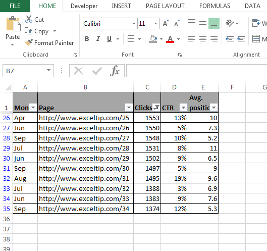
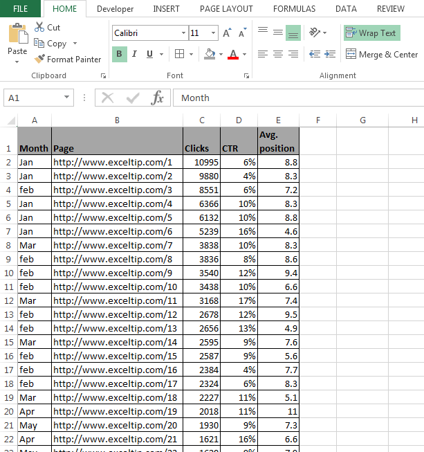
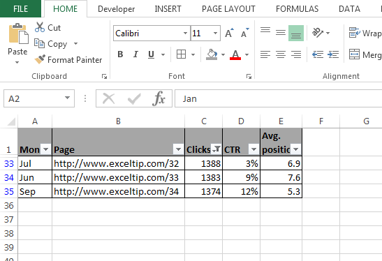
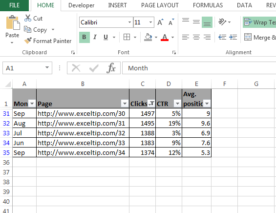
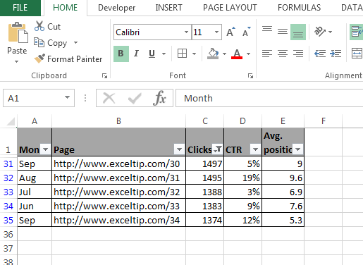
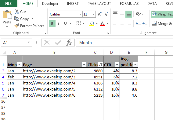
We have data in range A1:E35 in which column A contains Month, column B Page, column C Clicks, Column D CTR and column E contains average position.
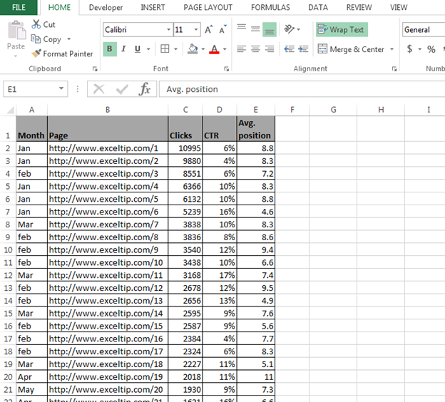
If we want to see the data of Jan month, then we need to put the filter on Jan month. To put the filter through VBA, follow below given steps:-
- Open VBA Page press the key Alt+F11.
- Insert a module.
- Write the below mentioned code:
Sub Filterindata()
Range(«A1″).AutoFilter Field:=1, Criteria1:=»Jan»
End Sub
Code Explanation:- Firstly, we have to select the range of data where we want to put the filter and then we need to define the criteria.
To run the macro, press the key F5, and data will get filtered and we can see only Jan data.

How to put the filter for bottom 10 items?
To understand how to put the filter for bottom 10 items, let’s take an example:-
We have data in range A1:E35 in which column A contains Month, column B Page, column C Clicks, Column D CTR and column E contains average position.

If we want to see the bottom 10 clicks in the data, then we need to follow below given steps:-
- Open VBA Page press the key Alt+F11.
- Insert a module.
- Write the below mentioned code:
Sub filterbottom10()
Range(«A1″).AutoFilter Field:=3, Criteria1:=»10», Operator:=xlBottom10Items
End Sub
Code Explanation:- First, we have to select the range of data where we want to put the filter and then we need to define the criteria to filter the data of bottom 10 items.
To run the macro, press the key F5, and data will get filtered and we can see only bottom10 click’s data.
How to put the filter for bottom 10 percent of data?
To understand how to put the filter for bottom 10 percent of data, let’s take an example:-
We have data in range A1:E35 in which column A contains Month, column B Page, column C Clicks, Column D CTR and column E contains average position.
If we want to see the bottom 10 percent data, then we need to follow below given steps:-
- Open VBA Page and press the key Alt+F11.
- Insert a module.
- Write the below mentioned code:
Sub Filterbottom10percent()
Range(«A1″).AutoFilter Field:=3, Criteria1:=»10», Operator:=xlBottom10Percent
End Sub
Code Explanation:- First, we have to select the range of data where we want to put the filter and then we need to define the criteria to filter the data of bottom 10 percent.
To run the macro, press the key F5, and data will get filtered and we can see only bottom10 percent data.
How to put the filter for bottom X number of Items of data?
To understand how to put the filter for bottom X numbers, let’s take an example:-
We have data in range A1:E35 in which column A contains Month, column B Page, column C Clicks, Column D CTR and column E contains average position.

If we want to see the bottom x number of data, then we need to follow below given steps:-
- Open VBA Page press the key Alt+F11.
- Insert a module.
- Write the below mentioned code:
Sub Filterbottomxnumber()
Range(«A1″).AutoFilter Field:=3, Criteria1:=»5», Operator:=xlBottom10Items
End Sub
Code Explanation:- First we have select the range of data where we want to put the filter and then we gave the criteria to filter the 5 numbers of bottom 10 numbers.
To run the macro press the key F5, data will get filtered and we can see only bottom 10 click’s data.
How to put the filter for bottom x percent of data?
To understand that how to put the filter for bottom x percent of data, let’s take an example:-
We have data in range A1:E35, in which column A contains Month, column B Page, column C Clicks, Column D CTR and column E contains average position.

If we want to see the bottom x percent data, then we need to follow below given steps:-
- Open VBA Page press the key Alt+F11.
- Insert a module.
- Write the below mentioned code:
Sub Filterbottomxpercent()
Range(«A1″).AutoFilter Field:=3, Criteria1:=»5», Operator:=xlBottom10Percent
End Sub
Code Explanation:- First we have to select the range of data where we want to put the filter and then we need to define the criteria to filter the data of bottom x percent.
To run the macro, press the key F5, and data will get filtered and we can see only bottom 10 Percent data.
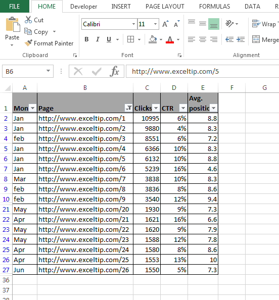
How to put the filter for specific text?
To understand how to put the filter for specific, let’s take an example:-
We have data in range A1:E35 in which column A contains Month, column B Page, column C Clicks, Column D CTR and column E contains average position.

If we want to see the specific data only in column B, then we need to follow below given steps:-
- Open VBA Page and press the key Alt+F11.
- Insert a module.
- Write the below mentioned code:
Sub Specificdata()
Range(«A1″).AutoFilter Field:=2, Criteria1:=»*Exceltip*»
End Sub
Code Explanation:- First we have select the range of data where we will define the column B in Field as 2 and then we will define that which data we want to see.
To run the macro press the key F5, data will get filtered and we can see only Exceltip’s data will appear.
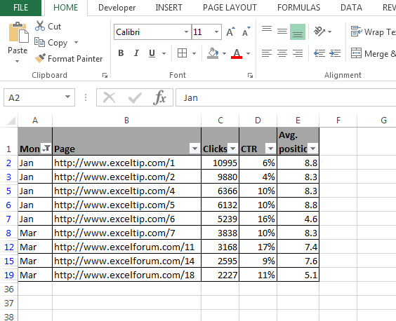
How to put the filter for multiple criteria?
To understand how to put the filter specifically, let’s take an example:-
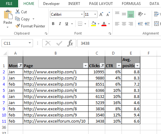
We have data in range A1:E35 in which column A contains Month, column B Page, column C Clicks, Column D CTR and column E contains average position.

If we want to see the data for Jan and Mar month, then we need to follow below given steps:-
- Open VBA Page press the key Alt+F11.
- Insert a module.
- Write the below mentioned code:
Sub Multipledata()
Range(«A1:E1″).AutoFilter field:=1, Criteria1:=»Jan», Operator:=xlAnd, Criteria2:=»Mar»
End Sub
Code Explanation:- First we have to select the range of data where we will define the column A in Field as 1 and then we will define the both criteria.
To run the macro, press the key F5, and data will get filtered and we can see only Jan and Mar data will appear.
How to put the filter to display the records that contain a value between 2 values?
To understand how to put the filter for multiple criteria, let’s take an example:-
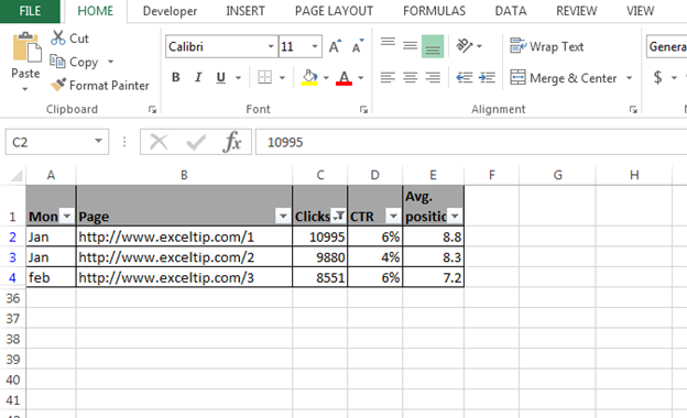
We have data in range A1:E35 in which column A contains Month, column B Page, column C Clicks, Column D CTR and column E contains average position.

If we want to put the filter as per the criteria how many numbers we have under the clicks of 5000 to 10000 , follow below given steps:-
- Open VBA Page and press the key Alt+F11.
- Insert a module.
- Write the below mentioned code:
Sub MultipleCriteria()
Range(«A1:E1″).AutoFilter field:=3, Criteria1:=»>5000″, Operator:=xlAnd, Criteria2:=»<10000″
End Sub
Code Explanation: — First we have to select the range of data where we will define the criteria in column C by using operator function.
To run the macro, press the key F5, and data will get filtered and we can see the data as per the clicks which is more than 5000 and less than 10000.
How to put the filter for multiple criteria in multiple columns?
To understand how to put the filter for multiple criteria in multiple columns, let’s take an example:-
We have data in range A1:E35 in which column A contains Month, column B Page, column C Clicks, Column D CTR and column E contains average position.

If we want to put the filter in Jan month to see that how many links are there in excel tips So we have to put the filter in Column A and B, follow below given steps:-
- Open VBA Page press the key Alt+F11.
- Insert a module.
- Write the below mentioned code:
Sub MultipleFields()
Range(«A1:E1″).AutoFilter field:=1, Criteria1:=»Jan»
Range(«A1:E1″).AutoFilter field:=2, Criteria1:=»*Exceltip*»
End Sub
Code Explanation: — Firstly, we have to select the range of data where we want to put the filter and then we will have to define the criteria 2 times to achieve the target.
To run the macro, press the key F5, and data will get filtered and we can see how many links belong to Exceltip in the data of Jan month.

How to filter the data without applying the filter arrow?
To understand how to filter the data without applying the filter in column, let’s take an example:-
We have data in range A1:E35 in which column A contains Month, column B Page, column C Clicks, Column D CTR and column E contains average position.

If we want to put the filter for in Jan month and hide the filter arrow in the field, follow below given steps:-
- Open VBA Page press the key Alt+F11.
- Insert a module.
- Write the below mentioned code:
Sub HideFilter()
Range(«A1″).AutoFilter field:=1, Criteria1:=»Jan», visibledropdown:=False
End Sub
Code Explanation: — First, we have to select the range of data where we want to put the filter and then we need to make sure that filter should not be visible.
To run the macro, press the key F5, and data will get filtered. Now, we can see the data in Jan month’s data only but the filter arrow will not appear in month’s column.
How to filter the data for displaying the 1 0r 2 Possible values?
To understand how to filter the data to display the 1 or 2 possible values, let’s take an example:-
We have data in range A1:E35 in which column A contains Month, column B Page, column C Clicks, Column D CTR and column E contains average position.

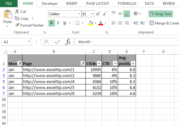
If we want to put the filter in Jan month and hide the filter arrow in the field, we need to follow below given steps:-
- Open VBA Page press the key Alt+F11.
- Insert a module.
- Write the below mentioned code:
Sub HideFilter()
Range(«A1″).AutoFilter field:=1, Criteria1:=»Jan», visibledropdown:=False
End Sub
Code Explanation: — Firstly, we have to select the range of data where we want to put the filter and then we will make sure that filter should not be visible.
To run the macro, press the key F5, and data will get filtered. Now, we can see the data in Jan month’s data and Feb month’s data.

How to put the filter for top 10 items?
To understand how to put the filter for top 10 items, let’s take an example:-
We have data in range A1:E35 in which column A contains Month, column B Page, column C Clicks, Column D CTR and column E contains average position.

If we want to see the top 10 clicks in the data, then we need to follow below given steps:-
- Open VBA Page and press the key Alt+F11.
- Insert a module.
- Write the below mentioned code:
Sub filtertop10()
Range(«A1″).AutoFilter Field:=3, Criteria1:=»10», Operator:=xlTop10Items
End Sub
Code Explanation- Firstly, we have to select the range of data where we want to put the filter and then we need to define the criteria to filter the data from top 10 items.
To run the macro, press the key F5, and data will get filtered and we can see only top 10 click’s data.
How to put the filter for top 10 percent of data?
To understand how to put the filter for top 10 percent of data, let’s take an example:-
We have data in range A1:E35 in which column A contains Month, column B Page, column C Clicks, Column D CTR and column E contains average position.

If we want to see the top 10 percent data, then we need to follow below given steps:-
- Open VBA Page press the key Alt+F11.
- Insert a module.
- Write the below mentioned code:
Sub Filtertop10percent()
Range(«A1″).AutoFilter Field:=3, Criteria1:=»10», Operator:=xlTop10Percent
End Sub
Code Explanation:- First we have to select the range of data where we want to put the filter and then we need to define the criteria to filter the data from top 10 percent.
To run the macro, press the key F5, and data will get filtered. Now, we can see only top 10 percent data.
How to remove the filter?
To understand how to remove the filter, follow below given steps:-
- Open VBA Page press the key Alt+F11.
- Insert a module.
- Write the below mentioned code:
Sub removefilter()
Worksheets(«Sheet1»).ShowAllData
End Sub
To run the macro press the key F5, all data will get show but filter arrow will not be remove.
This is all about how we can put the filters through VBA in Microsoft Excel.
![]()
In this Article
- Advanced Filter Syntax
- Filtering Data In Place
- Resetting the data
- Filtering Unique Values
- Using the CopyTo argument
- Removing Duplicates from the data
This tutorial will explain the how to use the Advanced Filter method in VBA
Advanced Filtering in Excel is very useful when dealing with large quantities of data where you want to apply a variety of filters at the same time. It can also be used to remove duplicates from your data. You need to be familiar with creating an Advanced Filter in Excel before attempting to create an Advanced Filter from within VBA.
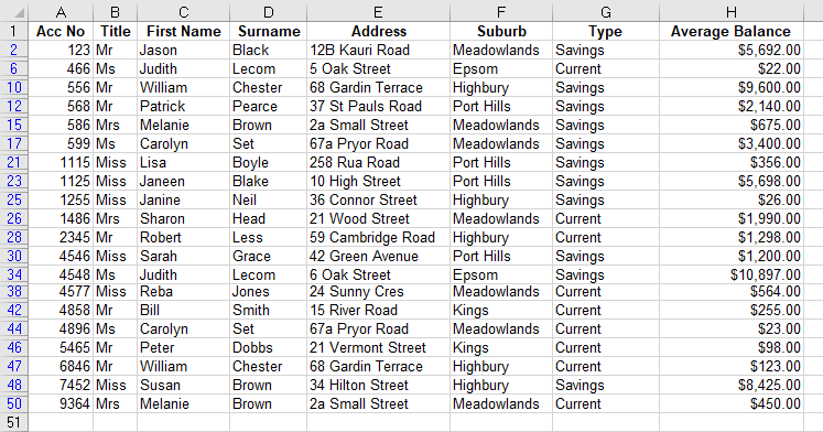
Consider the following worksheet.
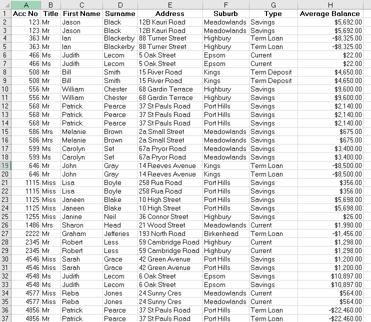
You can see at a glance that there are duplicates that you might wish to remove. The Type of account is a mixture of Saving, Term Loan and Check.
First you need to set up a criteria section for the advanced filter. You can do this in a separate sheet.
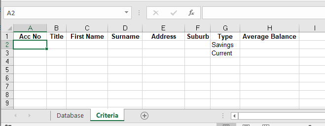
For ease of reference, I have named my data sheet ‘Database’ and my criteria sheet ‘Criteria’.
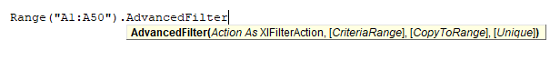
Advanced Filter Syntax
Expression.AdvancedFilter Action, CriteriaRange, CopyToRange, Unique
- The Expression represents the range object – and can be set as a Range (eg Range(“A1:A50”) – or the Range can be assigned to a variable and that variable can be used.
- The Action argument is required and will either be xlFilterInPlace or xlFilterCopy
- The Criteria Range argument is where you are getting the Criteria to filter from (our Criteria sheet above). This is optional as you would not need a criteria if you were filtering for unique values for example.
- The CopyToRange argument is where you are going to put your filter results – you can filter in place or you can have your filter result copied to an alternative location. This is also an optional argument.
- The Unique argument is also optional – True is to filter on unique records only, False is to filter on all the records that meet the criteria – if you omit this, the default will be False.
Filtering Data In Place
Using the criteria shown above in the criteria sheet – we want to find all the accounts with a type of ‘Savings’ and ‘Current’. We are filtering in place.
Sub CreateAdvancedFilter()
   Dim rngDatabase As Range
   Dim rngCriteria As Range
'define the database and criteria ranges
   Set rngDatabase = Sheets("Database").Range("A1:H50")
   Set rngCriteria = Sheets("Criteria").Range("A1:H3")
'filter the database using the criteria
   rngDatabase.AdvancedFilter xlFilterInPlace, rngCriteria
End Sub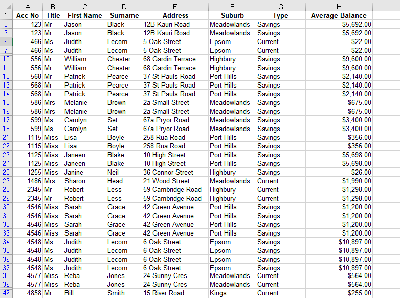
The code will hide the rows that do not meet the criteria.
In the above VBA procedure, we did not include the CopyToRange or Unique arguments.
Resetting the data
Before we run another filter, we have to clear the current one. This will only work if you have filtered your data in place.
Sub ClearFilter()
   On Error Resume Next
'reset the filter to show all the data
   ActiveSheet.ShowAllData
End Sub
Filtering Unique Values
In the procedure below, I have included the Unique argument but omitted the CopyToRange argument. If you leave this argument out, you EITHER have to put a comma as a place holder for the argument
Sub UniqueValuesFilter1()
   Dim rngDatabase As Range
   Dim rngCriteria As Range
'define the database and criteria ranges
   Set rngDatabase = Sheets("Database").Range("A1:H50")
   Set rngCriteria = Sheets("Criteria").Range("A1:H3")
'filter the database using the criteria
   rngDatabase.AdvancedFilter xlFilterInPlace, rngCriteria,,True
End Sub
OR you need to use named arguments as shown below.
Sub UniqueValuesFilter2()
   Dim rngDatabase As Range
   Dim rngCriteria As Range
'define the database and criteria ranges
   Set rngDatabase = Sheets("Database").Range("A1:H50")
   Set rngCriteria = Sheets("Criteria").Range("A1:H3")
'filter the database using the criteria
   rngDatabase.AdvancedFilter Action:=xlFilterInPlace, CriteriaRange:=rngCriteria, Unique:=True
End Sub
Both of the code examples above will run the same filter, as shown below – the data with only unique values.
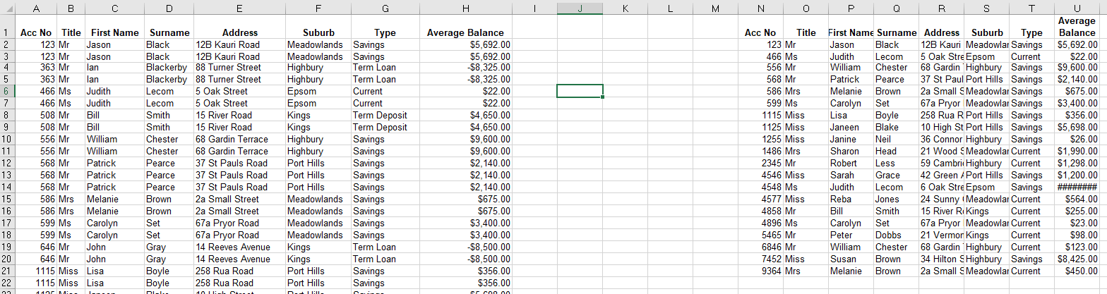
Using the CopyTo argument
Sub CopyToFilter()
   Dim rngDatabase As Range
   Dim rngCriteria As Range
'define the database and criteria ranges
   Set rngDatabase = Sheets("Database").Range("A1:H50")
   Set rngCriteria = Sheets("Criteria").Range("A1:H3")
'copy the filtered data to an alternative location
    rngDatabase.AdvancedFilter Action:=xlFilterCopy, CriteriaRange:=rngCriteria, CopyToRange:=Range("N1:U1"), Unique:=True
End Sub
Note that we could have omitted the names of the arguments in the Advanced Filter line of code, but using named arguments does make the code easier to read and understand.
This line below is identical to the line in the procedure shown above.
rngDatabase.AdvancedFilter xlFilterCopy, rngCriteria, Range("N1:U1"), TrueOnce the code is run, the original data is still shown with the filtered data shown in the destination location specified in the procedure.
Removing Duplicates from the data
We can remove duplicates from the data by omitting the Criteria argument, and copying the data to a new location.
Sub RemoveDuplicates()
   Dim rngDatabase As Range
'define the database
   Set rngDatabase = Sheets("Database").Range("A1:H50")
'filter the database to a new range with unique set to true
rngDatabase.AdvancedFilter Action:=xlFilterCopy, CopyToRange:=Range("N1:U1"), Unique:=True
End Sub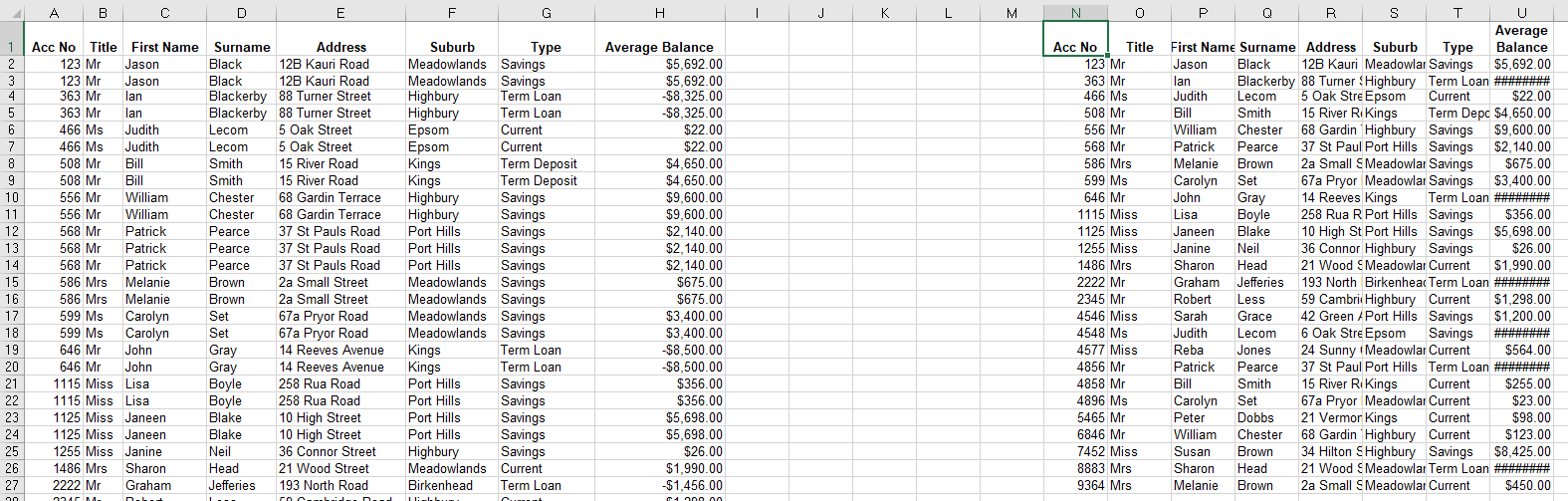
VBA Coding Made Easy
Stop searching for VBA code online. Learn more about AutoMacro — A VBA Code Builder that allows beginners to code procedures from scratch with minimal coding knowledge and with many time-saving features for all users!

Learn More!
Фильтрация одномерного массива в VBA Excel с помощью функции Filter. Синтаксис и параметры функции Filter. Пример фильтрации одномерного массива.
Filter – это функция, которая возвращает массив, содержащий строки исходного одномерного массива, соответствующие заданным условиям фильтрации.
Примечания
- исходный (фильтруемый) массив должен быть одномерным и содержать строки;
- индексация возвращенного массива начинается с нуля;
- возвращенный массив содержит ровно столько элементов, сколько строк исходного массива соответствуют заданным условиям фильтрации;
- переменная, которой присваивается возвращенный массив, должна быть универсального типа (As Variant) и объявлена не как массив (не myArray() со скобками, а myArray без скобок).
Функция Filter автоматически преобразует обычную переменную универсального типа, которой присваивается отфильтрованный список, в одномерный массив с необходимым количеством элементов.
Синтаксис
|
Filter(sourcearray, match, [include], [compare]) |
Параметры
| Параметр | Описание |
|---|---|
| sourcearray | Обязательный параметр. Одномерный массив, элементы которого требуется отфильтровать |
| match | Обязательный параметр. Искомая строка. |
| include | Необязательный параметр. Значение Boolean, которое указывает:
|
| compare | Необязательный параметр. Числовое значение (константа), указывающее тип сравнения строк. По умолчанию – 0 (vbBinaryCompare). |
Compare (значения)
Параметр compare может принимать следующие значения:
| Константа | Значение | Описание |
|---|---|---|
| vbUseCompareOption | -1 | используется тип сравнения, заданный оператором Option Compare |
| vbBinaryCompare | 0 | выполняется двоичное сравнение (регистр имеет значение) |
| vbTextCompare | 1 | выполняется текстовое сравнение (без учета регистра) |
Пример фильтрации
Фильтрация списка в столбце «A» по словам, начинающимся с буквы «К», и загрузка результатов в столбец «B»:

Пример кода VBA Excel с функцией Filter:
|
1 2 3 4 5 6 7 8 9 10 11 12 13 14 15 16 17 |
Sub Primer() Dim arr1, arr2, arr3, i As Long ‘Присваиваем переменной arr1 массив значений столбца A arr1 = Range(«A1:A» & Range(«A1»).End(xlDown).Row) ‘Копируем строки двумерного массива arr1 в одномерный arr2 ReDim arr2(1 To UBound(arr1)) For i = 1 To UBound(arr1) arr2(i) = arr1(i, 1) Next ‘Фильтруем строки массива arr2 по вхождению подстроки «К» ‘и присваиваем отфильтрованные строки переменной arr3 arr3 = Filter(arr2, «К») ‘Копируем строки из массива arr3 в столбец «B» For i = 0 To UBound(arr3) Cells(i + 1, 2) = arr3(i) Next End Sub |
What is VBA?
VBA is a programming language that can automate tasks within Excel using macros. You can calculate, move and manipulate data using this language. This is particularly useful for repetitive tasks that don’t have a single formula fix.
If you’re looking for more background, check out this video on the differences between macros and VBA.
If you already have some experience creating macros, this article will show you how to take your skills to the next level with the Excel VBA advanced filter.
Step up your Excel game
Download our print-ready shortcut cheatsheet for Excel.
What is advanced filtering?
VBA advanced filtering is used for more complex filtering needs that the AutoFilter in Excel cannot complete.
You can filter out unique items, extract specific words or dates and even copy them to another document or sheet. In this article, we will be using VBA to control advanced filtering – but first, we need to show you how to build and setup your document so it is ready for VBA advanced filtering.
How to set up advanced filtering
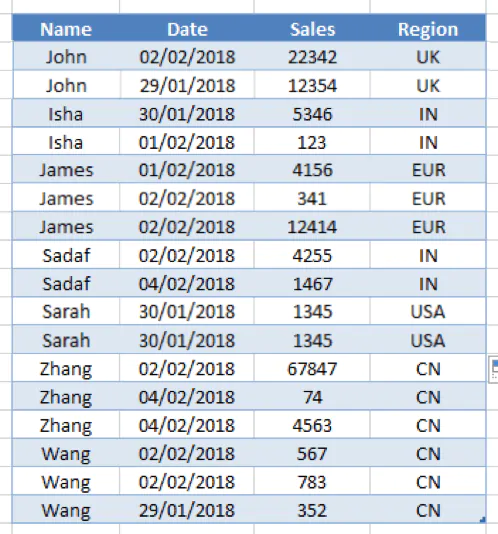
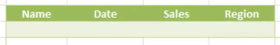
Here are the steps for setting up the data ready for advanced filtering. I will be using a blue table for the Data Range, and green for the Criteria Range, as shown in the screenshots below.
Database
- Set up a table or arrangement of data with header names
- Each header needs a unique name otherwise it will cause issues when filtering
- The rows below the headers should contain the data you wish to filter
- No blank rows can be in the data set (apart from the last row at the bottom)
Criteria Range
The criteria range are the rules that will be applied to the data when using the VBA Advanced Filter. You can set one or multiple criteria.
- This can be set up as a range of cells or as a table
- To set up a table, simply select the range of cells including the headers and click Insert → Table
- You can rename your table by clicking anywhere on the new table and editing the text where it says ‘Table1’
- Note: The headers need to match the headers from the database exactly
- You don’t need to have every header – just the ones you want to filter by
-
You can use operators within the cell such as:
- < Less than
- > Greater than
- >= Greater than or equal to
- <= Less than or equal to
- <> Not equal to
For example, <1000 in the cell would return items that are less than 1000
Extract Range
This tool allows you to set an area of data to copy or move. This is particularly useful if, for example, you want to export out a list of contacts or locations. To set this up:
- The same rule applies here as the criteria range; the headers need to be exactly the same
- Note: The headers don’t need to be in the same order and you don’t have to filter all of the columns – just the ones you want to see. For example, if you wanted just a list of names then you would have only the ‘Name’ column on your chosen extract sheet.
Apply the advanced filter
This is to set the area you want to copy the filtered items to.
- Select any cell in the database
- On the Excel Ribbon Data tab, click advanced filtering
- You can choose to filter in place or to another location, depending on how you want to extract the data
- Set the criteria range
- Note: When copying to another location Excel will clear any data already stored in your extract location when the filter is applied
- Click OK
Filtering unique items
There is an option when filtering to only return unique items. This will return only 1 record that meets each of the criteria you have set. To do this:
-
Simply tick the unique box when filtering
Setting up VBA
Advanced filtering is all well and good, but we have to click ‘advanced filter’ every time we want to filter the list down. This is fine, but it’s not why you came to this article!
First, we need to access the Visual Basic screen in Excel – by default, this is turned off. To turn it on go to:
- File → Options → Ribbon Settings and turn on the Developer tab
- This should turn on an extra tab in Excel so you can create, record and modify VBA code using Macros.
- There are a few kinds of Macros – we will cover:
- Macros that run by clicking on a button
- Macros that run when a cell or range is modified
Button VBA macro
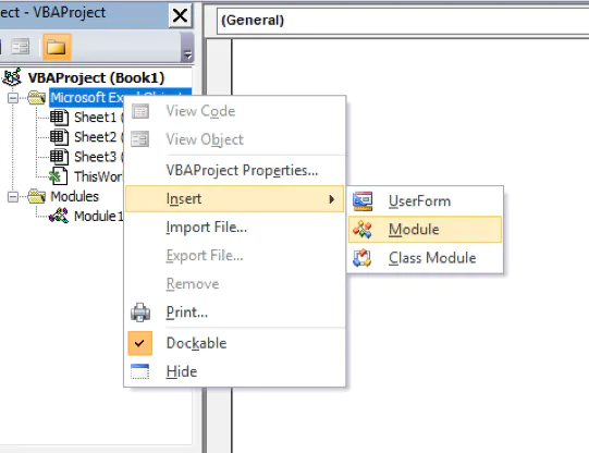
To create a button that triggers a VBA macro we need to create a ‘Module’ within VBA. To do this:
- Navigate to the Developer tab and click on ‘Visual Basic’
- Right-click on ‘Excel Objects Folder’ and click ‘Create New Module’:
Once you’ve created the new module we can start writing a Macro:
- We always start with Sub NameOfTheSubroutine () and end with End Sub
- We would write our code in-between those lines. For example:
Sub Advanced Filtering ()
End Sub
Here is the start of our VBA code that would go in between the lines above:
- The «Database» would be replaced with the range area of our data
- The «Criteria» would be replaced by our Criteria range
Range("Database").AdvancedFilter _
Action:=xlFilterInPlace, _
CriteriaRange:=Range("Criteria")
VBA Code so far:
Sub Advanced_Filtering()

Range("C6:F23").AdvancedFilter _
Action:=xlFilterInPlace, _
CriteriaRange:=Range("C2:F3")

End Sub
We now need to add a button:
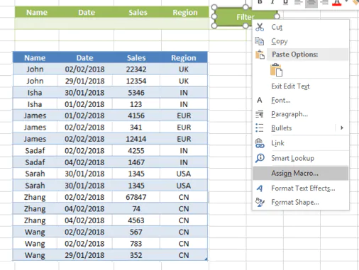
- Insert → Shape → Pick a Shape and draw it onto the sheet. In this case, we’ll use a rectangle.
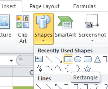
- Assign the Macro you have just created by right-clicking on the shape → Assign Macro. Test it by typing in the criteria range and click the button you’ve just added
Automatic VBA macro
We’ve just created a button to trigger our macro, but that’s an extra step – we want the list to just filter when we enter something into those cells. To do this we can use Worksheet_Change to trigger the Macro we have just created to run when we update the criteria changes.
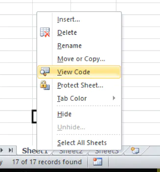
-
Right-click on the sheet and click ‘View Code’ – if this doesn’t work you can access via Visual Basic view on the Developer tab. Then double-click on the sheet with your criteria range on it (In this example it’s sheet 1).
Another way to trigger a VBA Macro is to get Excel to automatically trigger whenever a sheet is updated — In other words when you add, update or change a cell.
This is great, but we don’t want Excel to trigger the code when any cell is updated — We only want to trigger the Macro when a specific range is updated.
- The code below will first check to see if the cells updated are C3 to F3 (our criteria range) and if it’s not it will kill the subroutine (Then Exit Sub).
- If it is within those cells, it triggers our first Macro to run
- This is useful and important as will only allow the code to run when we edit those cells
- If we didn’t have the ‘If Intersect’, it would run every time any cell is changed
Private Sub Worksheet_Change(ByVal Target As Range)

If Intersect(Target, Range("C3:F3")) Is Nothing Or Target.Cells.Count > 1 Then Exit Sub
Call Advanced_Filtering

End Sub
VBA copy to a new location
To alter the VBA to copy to a new location we simply need to change 2 parts of the code:
- We need to change Action:=xlFilterInPlace to Action:=xlFilterCopy
- And add CopyToRange:=Sheets(«SHEET NAME»).Range(«RANGE») to the end
- Here’s what the final code should look like. This will filter the data from Sheet 1 into Sheet 1 in the range A1:D1:
Sub Advanced_Filtering()

CriteriaLastRow = 4 'Last Row you have in the Criteria range

For i = 3 To CriteriaLastRow 'Loops through until the last Row
  RowsCount = Application.WorksheetFunction.CountA(Range("C" & i & ":F" & i))
  If RowsCount = 0 Then CriteriaRowsSet = i - 1 Else CriteriaRowsSet = CriteriaLastRow 'Checks to see if any row returns 0 and sets it to the row above's number
Next i

Range("C6:F23").AdvancedFilter _
Action:=xlFilterInPlace, _
CriteriaRange:=Range("C2:F" & CriteriaRowsSet), _ CopyToRange:=Sheets("Sheet2").Range("A1:D1")

End Sub
What we have gone through so far just covers the basics of filtering, but there is much more filtering is capable of. Let’s take a look at VBA advanced filtering with multiple criteria and wildcards.
Advanced filtering with multiple criteria
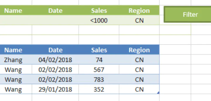
Currently, the criteria range can only handle AND statements – meaning it would need to meet all of the criteria to display after filtering. If I wanted to do an OR statement (i.e. I want to show results that are either Wang OR John) then I would need to expand my criteria table:
- First I would expand my row at the bottom to allow for more statements
- Expand both Macros to allow for the extra row
- Note: Make sure when moving or adding new rows that the Macros are still looking at the correct range. Macros are not like formulas that automatically change when you add new rows
- If you do need to add/remove cells then you would need to go back into the VBA code and extend or shorten the range of cells within the code.
If we wanted to remove a column, for example, we would change this code:
Range("C6:F23").AdvancedFilter _
Action:=xlFilterInPlace, _
CriteriaRange:=Range("C2:F" & CriteriaRowsSet), _
CopyToRange:=Sheets("Sheet2").Range("A1:D1")
To this code:
Range("C6:E23").AdvancedFilter _
Action:=xlFilterInPlace, _
CriteriaRange:=Range("C2:E" & CriteriaRowsSet), _
CopyToRange:=Sheets("Sheet2").Range("A1:D1")
Notice I changed both the Filter area and the range Criteria. This is showing me records that are for Wang AND 2/2/2018 OR John: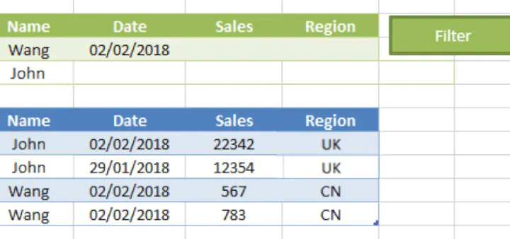
Note: This will not work unless something is contained within both rows or all of the rows if you have more. So we will need to add some code to find which is the bottom row:
- The code below starts off and sets the last row to 4 (meaning the last row number for your criteria)
- It then loops through and checks each row from 3 to your last row and counts how many items are in there
- If it gets right to the bottom and nothing is 0 it sets the criteria range to your full criteria data
- If it returns a 0 on any line it sets the range to the row above it
Sub Advanced_Filtering()

CriteriaLastRow = 4 'Last Row you have in the Criteria range

For i = 3 To CriteriaLastRow 'Loops through until the last Row
  RowsCount = Application.WorksheetFunction.CountA(Range("C" & i & ":F" & i))
  If RowsCount = 0 Then CriteriaRowsSet = i - 1 Else CriteriaRowsSet = CriteriaLastRow 'Checks to see if any row returns 0 and sets it to the row above's number.
Next i

  Range("C6:F23").AdvancedFilter _
  Action:=xlFilterInPlace, _
  CriteriaRange:=Range("C2:F" & CriteriaRowsSet)

End Sub
Advanced filtering with wildcards
Wildcard filtering is where we use a special character to replace a letter to give us similar results.
To use a Wildcard we wouldn’t need to amend any data or VBA code. We would use a symbol within the search criteria.
- The asterisk (*) wildcard character represents any number of characters in that position, including zero characters.
- The question mark (?) wildcard character represents one character in that position.
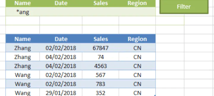
For example, *ang would return anything that ended with the letters ang:
In summary
So, what have we learned?
- That almost any task/function in Excel can be automated using VBA
- How to filter down data more precisely and accurately using VBA
- How to filter down by wildcards
- How to move our filtered data to another location
- How to filter using multiple criteria
- The basics of being able to loop through data and perform a function on each line. This is not just limited to advanced filtering as it can be used with other Excel functions
- The different triggers for VBA in Excel:
- Button – A Macro will run on a click of a button
- Call – A Macro will be ‘called’ (triggered) from another Macro
- Change – A Macro will run when a sheet is updated
This tutorial only covers a small portion of the capability VBA and Macros have in Excel. If you’d like to learn more about creating powerful macros to automate your tasks, check out our Macros and VBA course.
Now that you’ve got filtering down pat, why don’t you try creating your own user defined functions? Learn from the pros with our step-by-step guide on how to build Excel UDFs.
Ready to become a certified Excel ninja?
Take GoSkills’ Macros & VBA course today!
Start free trial
VBA Advanced Filter is one of the many hidden gems that Excel VBA offers to make our time more productive.
VBA Advanced Filter requires very little code, is one of the fastest ways to copy data, and provides advanced filtering options that we cannot get anywhere else.
VBA Advanced Filter Quick Guide
Using the criteria with AdvancedFilter is very powerful. You can see the possible options in the table below:
| Task | Cell formula | Examples where true |
|---|---|---|
| Contains | Pea =»Pea» =»*Pea*» |
Peach, Pea, Appear |
| Does not contain | =»<>*Pea*» | any text that does not contain Pea |
| Exact match | =»=Pea» | Pea |
| Does not exactly match | =»<>Pea» | Peach, Pear etc. |
| Starts with | =»=Pea*» | Peach, Pear, Pea |
| Ends with | =»=*Pea» | SweetPea, GreenPea |
| Use the ? symbol to represent any single character | =»=Pea?» | Pear, Peas or any 4 letter word starting with «Pea» |
| Any of the symbols *?~ | =»=Pea~*» | Pea*, Pea? |
| Case sensitive(see section Using Formulas as Criteria) | =EXACT(A7,»Peach») | Peach |
| Greater than | =»>700″ | 701,702 etc. |
| Greater than or equals | =»>=700″ | 700, 701,702 etc. |
| Less than | =»<700″ | 699,698 etc. |
| Less than or equals | =»<=700″ | 700, 699, 698 etc. |
| Equals | =»=700″ | 700 |
Important Note: A Criteria column header must exist as a List range column header. For example, if the Criteria column header is “Fruit” then there must be a List range column header called “Fruit”.
Here are some important things to know about the Criteria column headers:
- They can be used in any order.
- You can use the same header multiple times(see section Advanced Filter Multiple Criteria below).
- You don’t need to include a column header in the criteria if you are not filtering by this column.
What is Advanced Filter
Advanced Filter is a tool that is available in the Sort & Filter section of the Data tab on the Excel Ribbon:

It allows us to filter data based on a Criteria range. This allows us to do more advanced filtering than the standard filtering on the worksheet.
A second advantage of using Advanced Filter is that we have the option to copy the results to a new range if we choose.
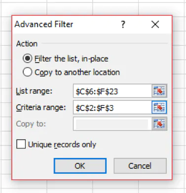
Using Advanced Filter is quite simple as you can see from the dialog:

We filter in-place or we copy to another location. We then simply need the data range(List range) and the Criteria Range. If we decided to copy to another location then we provide the “Copy to” range.
Using Advanced Filter is very useful in VBA because it is extremely fast, powerful and as we will see it requires very little code.
VBA Advanced Filter on YouTube
To see me working with Advanced Filter, check out this YouTube video:
VBA Advanced Filter Parameters
The following table shows the parameters of the AdvancedFilter function:
| Parameter | Optional | Type | Details |
|---|---|---|---|
| Action | Required | xlFilterAction | xlFilterInPlace or xlFilterCopy. |
| CriteriaRange | Optional | Range | Range of the criteria used for filtering the data. |
| CopyToRange | Optional | Range | Destination range if Action is set to xlFilterCopy. |
| Unique | Optional | Boolean | True for unique records only. |
You can read about the parameters on the Microsoft help page.
AdvancedFilter requires three ranges to run(or two if you are using xlFilterInPlace as the Action parameter):
- List range – data to filter.
- Criteria range – how to filter.
- Copy To range – where to place the results if the Action parameter is set to xlFilterCopy is set.
AdvancedFilter is a range Function. This means you get the range of data you wish to filter and then call the AdvancedFilter function of that range:
DataRange.AdvancedFilter Filter Action, Criteria, [CopyTo], [Unique]
We can filter in place or we can copy the filter results to another location. This means there are two ways to use AdvancedFilter:
 ' Filter in place
 rgData.AdvancedFilter xlFilterInPlace, rgCriteriaRange

 ' Filter and copy data
 rgData.AdvancedFilter xlFilterCopy, rgCriteriaRange, rgDestination
The first parameter indicates the way to apply the filter:
- xlFilterInPlace – Filter the original data.
- xlFilterCopy – Copy the filter results to a new range.
If we use xlFilterInPlace then we don’t need the destination range.
To remove duplicate records we simply set the Unique parameter to True. Otherwise, duplicate records are ignored:
 ' Filter in place
 rgData.AdvancedFilter xlFilterInPlace, rgCriteriaRange, , True

 ' Filter and copy data
 rgData.AdvancedFilter xlFilterCopy, rgCriteriaRange, rgDestination, True
Understanding the Advanced Filter Ranges
The following screenshot shows an example of the 3 ranges. The List(or data) range is shaded blue, the Criteria range is green, and the CopyTo range is yellow:

The following subsection provides a quick guide to each of the ranges:
Criteria Range
- The criteria headers must be one of the List Range column headers. If not then it will be ignored.
- Criteria headers can be in any order.
- You can include as many or as few Criteria headers as you need.
- You can use the same header multiple times – this allows us to do multiple AND operations on the same column.
CopyTo Range
- This range is only used when the Action parameter is set to xlFilterCopy.
- To avoid errors this range should be the Header row of the output destination.
- You can use any(or all) columns from the List range as your output and they can be in any order.
- The columns headers in this range must be a List Range column header or you will get a VBA Runtime Error 1004.
List Range
- The List Range is the range of data that will be filtered.
- You must include the headers as part of the List Range.
- If you set the Action parameter to xlFilterInPlace then the List data will be filtered.
- If you set the Action parameter to xlFilterCopy then the results will be copied to the location which is specified in the CopyToRange parameter.
Writing the VBA Code
The easiest way to define the data range is to use CurrentRegion although you can get the range any way you like. Using CurrentRegion gets all the adjacent data to the specified cell or range.
We can use CurrentRegion like this:
 Dim rgData As Range, rgCriteriaRange As Range
 Set rgData = Range("A4").CurrentRegion
 Set rgCriteriaRange = Range("A1").CurrentRegion
To set the CopyTo range, you specify the entire heading row.
You can use a simple trick with CurrentRegion to get the CopyToRange header row. First, use CurrentRegion and then take the first row of the resulting range:
 Dim rgCopyToRange As Range
 Set rgCopyToRange = shFruit.Range("E4").CurrentRegion.Rows(1)
The full VBA Advanced filter code looks like this:
Sub RunAdvancedFilter()

    ' Declare the variables
    Dim rgData As Range, rgCriteriaRange As Range, rgCopyToRange As Range

    ' Set the ranges
    Set rgData = Sheet1.Range("A4").CurrentRegion
    Set rgCriteriaRange = Sheet1.Range("A1").CurrentRegion
    Set rgCopyToRange = Sheet1.Range("D1").CurrentRegion.Rows(1)

    ' Run AdvancedFilter
    rgData.AdvancedFilter xlFilterCopy, rgCriteriaRange, rgCopyToRange

End Sub
You can run this code for pretty much any AdvancedFilter that you want to do. All you need to do is to change the ranges as appropriate. You can change Sheet1 in the code to any worksheet variable or code name.
Important Note: When we run AdvancedFilter using VBA, the ranges do not need to be on the same worksheet or even in the same workbook.
VBA Advanced Filter Clear
If we Filter the data in place then we can use ShowAllData to remove the filter. We should check the filter is turned on first so we don’t get an error. We can use the following code to check and clear the filter if it exists:
If Sheet1.FilterMode = True Then
    Sheet1.ShowAllData
End If
If we are we filter using copy then Advanced Filter will automatically remove existing data from the destination before copying. However, if you want to simply clear the data you can do it like this:
Sheet1.Range("E7").CurrentRegion.Offset(1).ClearContents
This highlights all the adjacent data to the output headers. It moves down one row using Offset to avoid clearing the header row.
VBA Advanced Filter Criteria
Check out this YouTube video to see me using Advanced Filter Criteria:
To use Criteria on a filter we use the columns headers of the List range with the criteria below them. The following criteria will return all rows where the Fruit column contains the text Orange:

This criteria will return the following rows:

Advanced Filter Multiple Criteria
We can use the columns in any row to filter by multiple criteria. This allows us to filter using AND logic e.g. If Fruit equals “Apple” AND City equals “New York”:

We can use multiple rows if we want to filter using OR logic e.g. If Fruit equals “Apple” OR Fruit equals “Pear” OR Fruit equals “Plum”:

Let’s have a look at examples of using Multiple Criteria with Advanced Filter:
Advanced Filter Multiple Criteria Examples
In our first example we will start with a simple AND filter:

These criteria return all the rows that have the fruit Orange AND the city Berlin:

In our next example, we are looking for a city that starts with S AND has sales of less than 500:

These criteria will return the following rows:

We can use any column header multiple times in the criteria range. For example, we can use the Sales column twice to get a number between 300 and 500:

These criteria will return the following rows:

Advanced Filter Criteria – OR
We use columns in a row when we want to do an AND operation. If we want want to do an OR operation we use rows in the Criteria filter.
In the following example we want to return rows where the Fruit is either a Peach OR a Banana:

This will return the following rows:

In the following example, we want to return any rows that have a fruit Banana OR sales that are greater than 900:

These criteria will return the following rows:

Combining AND Criteria and OR Criteria
Let’s look at an example of combining AND criteria with OR criteria.
This criteria filters by rows where (Fruit is Lemon AND City is Singapore) OR (Fruit is Orange AND City is Paris):

These are the results:

Using Formulas as Criteria
While the standard criteria methods offer powerful filtering methods they have limitations. The beauty of the AdvancedFilter is that we can use worksheet formulas in the criteria.
There are 3 rules when using formulas in the criteria range:
- No heading.
- The formula must result in True or False.
- The formula should reference the first row of the data range.
Imagine we have the following data:

We want to filter by games where the total number of goals scored was 2. We cannot do this using the normal criteria so we create a formula:
=B5+D5=2
We place this formula in cell A2:

You can see that we have followed the rules above:
- We have no header in the criteria.
- The result of the formula is False.
- The formula refers to the first row of the data i.e. B5 and D5.
The rows we get back are:

Note: If we want to use a formula on another row in the Criteria we should still refer to the first row of the data e.g.:
Cell A2 formula: =B5+D5=2
Cell A3 formula: =B5+D5=5
Cell A3 formula: =B5+D5=7
Advanced Filter Case Sensitive Criteria
There isn’t a simple way to use case sensitivity in our Criteria therefore we use a formula instead:
=EXACT(A5, “Pea”)
Make sure to follow the Formula rules in the previous section to ensure this works correctly.
VBA Advanced Filter Dates
Take a look at the following formula for the date criteria:
=”<1/9/2021″
This formula will work fine when we run Advanced Filter from the ribbon. But if we run Advanced Filter using VBA it will not return any records.
Instead, we have to use a formula like this:
=”<” & DATE(2021,9,1)
When we use this in the criteria like this:

we get:

If you want to do between dates then you can use the formulas in two columns. For example, imagine we want to get all the records in August 2021, then we can use the following formulas:
A2: =”<=” & DATE(2021,8,31)
B2: =”>=” & DATE(2021,8,1)

This will return the following rows:

VBA Advanced Filter Advantages and Limitations
Advanced Filter is easy to use and does its job very well. However, like every tool it has advantages and limitations to what it can do.
The following are the advantages of using the Advanced Filter:
- Speed – It is the fastest VBA method for copying and filtering data although multiple calls will slow it down.
- Advanced filtering – provides in-depth filtering options including the use of formulas.
- Requires very little code – You can use the same code most of the time and it’s simplistic compared to other methods of copying and filtering code in VBA.
- Formatting – When copying the results it automatically formats the result data to match the original data.
The following are the limitations of the Advanced Filter which you should be aware of:
- Speed – using AdvancedFilter is extremely fast but calling it multiple times in the same code, will cause it to run slower.
- Criteria can only use ranges – you cannot use an array for the Criteria. The workaround is to write the array to a range and then use it as the Criteria.
- Cannot alter data – AdvancedFilter simply filters and copies the data. You cannot make changes to the data after filtering and before copying.
- Cannot append data – To append data you need to write extra code.
Error 1004 – Extract Range
The most common error with the advanced filter is: Error 1004 – the extract range has a missing or invalid field name.
VBA Runtime Error 1004 occurs when one or more of the output column headers do not exist in the original data as we can see in this example:

If this error occurs you should ensure that the CopyTo range has the correct column headers with the correct spelling and that it is referencing the correct range.
What to do if Advanced Filter is not working
In general, when Advanced Filter throws an error, the problem is in one of the ranges.
If you have an error the following checks should fix most if not all errors:
- Ensure all the range variables are referencing the expected ranges.
- Ensure the Criteria and CopyTo column headers are correctly spelled and exist in the column headers of the List range.
- Ensure that the CopyTo range references the header row only.
- Ensure that any Criteria columns using formulas do not have a header.
- Make sure that there are no trailing spaces in Criteria.
TIP: If you are debugging the code you can check any range using the Address property of the range:

Wrapping Up
In this post, we’ve seen how to configure the ranges in a worksheet to be able to use Advanced Filter. We’ve also seen how, with a few lines of VBA code, we can take advantage of the power and speed of this function to filter and copy data.
We’ve also seen how to use the criteria to apply simple and complex filters and how to proceed when an error prevents us from using Advanced Filter.
Leave your comments if you want to know more about this powerful tool Excel gives us. Or if you’ve run into problems that prevent you from unleashing all its power.
What’s Next?
Free VBA Tutorial If you are new to VBA or you want to sharpen your existing VBA skills then why not try out this Free VBA Tutorial.
Related Training: Get full access to the Excel VBA training webinars and all the tutorials.
(NOTE: Planning to build or manage a VBA Application? Learn how to build 10 Excel VBA applications from scratch.)