
Присвоение диапазона ячеек объектной переменной в VBA Excel. Адресация ячеек в переменной диапазона и работа с ними. Определение размера диапазона. Примеры.
Присвоение диапазона ячеек переменной
Чтобы переменной присвоить диапазон ячеек, она должна быть объявлена как Variant, Object или Range:
|
Dim myRange1 As Variant Dim myRange2 As Object Dim myRange3 As Range |
Чтобы было понятнее, для чего переменная создана, объявляйте ее как Range.
Присваивается переменной диапазон ячеек с помощью оператора Set:
|
Set myRange1 = Range(«B5:E16») Set myRange2 = Range(Cells(3, 4), Cells(26, 18)) Set myRange3 = Selection |
В выражении Range(Cells(3, 4), Cells(26, 18)) вместо чисел можно использовать переменные.
Для присвоения диапазона ячеек переменной можно использовать встроенное диалоговое окно Application.InputBox, которое позволяет выбрать диапазон на рабочем листе для дальнейшей работы с ним.
Адресация ячеек в диапазоне
К ячейкам присвоенного диапазона можно обращаться по их индексам, а также по индексам строк и столбцов, на пересечении которых они находятся.
Индексация ячеек в присвоенном диапазоне осуществляется слева направо и сверху вниз, например, для диапазона размерностью 5х5:
| 1 | 2 | 3 | 4 | 5 |
| 6 | 7 | 8 | 9 | 10 |
| 11 | 12 | 13 | 14 | 15 |
| 16 | 17 | 18 | 19 | 20 |
| 21 | 22 | 23 | 24 | 25 |
Индексация строк и столбцов начинается с левой верхней ячейки. В диапазоне этого примера содержится 5 строк и 5 столбцов. На пересечении 2 строки и 4 столбца находится ячейка с индексом 9. Обратиться к ней можно так:
|
‘обращение по индексам строки и столбца myRange.Cells(2, 4) ‘обращение по индексу ячейки myRange.Cells(9) |
Обращаться в переменной диапазона можно не только к отдельным ячейкам, но и к части диапазона (поддиапазону), присвоенного переменной, например,
обращение к первой строке присвоенного диапазона размерностью 5х5:
|
myRange.Range(«A1:E1») ‘или myRange.Range(Cells(1, 1), Cells(1, 5)) |
и обращение к первому столбцу присвоенного диапазона размерностью 5х5:
|
myRange.Range(«A1:A5») ‘или myRange.Range(Cells(1, 1), Cells(5, 1)) |
Работа с диапазоном в переменной
Работать с диапазоном в переменной можно точно также, как и с диапазоном на рабочем листе. Все свойства и методы объекта Range действительны и для диапазона, присвоенного переменной. При обращении к ячейке без указания свойства по умолчанию возвращается ее значение. Строки
|
MsgBox myRange.Cells(6) MsgBox myRange.Cells(6).Value |
равнозначны. В обоих случаях информационное сообщение MsgBox выведет значение ячейки с индексом 6.
Важно: если вы планируете работать только со значениями, используйте переменные массивов, код в них работает значительно быстрее.
Преимущество работы с диапазоном ячеек в объектной переменной заключается в том, что все изменения, внесенные в переменной, применяются к диапазону (который присвоен переменной) на рабочем листе.
Пример 1 — работа со значениями
Скопируйте процедуру в программный модуль и запустите ее выполнение.
|
1 2 3 4 5 6 7 8 9 10 11 12 13 14 15 16 17 18 19 20 21 22 23 24 25 |
Sub Test1() ‘Объявляем переменную Dim myRange As Range ‘Присваиваем диапазон ячеек Set myRange = Range(«C6:E8») ‘Заполняем первую строку ‘Присваиваем значение первой ячейке myRange.Cells(1, 1) = 5 ‘Присваиваем значение второй ячейке myRange.Cells(1, 2) = 10 ‘Присваиваем третьей ячейке ‘значение выражения myRange.Cells(1, 3) = myRange.Cells(1, 1) _ * myRange.Cells(1, 2) ‘Заполняем вторую строку myRange.Cells(2, 1) = 20 myRange.Cells(2, 2) = 25 myRange.Cells(2, 3) = myRange.Cells(2, 1) _ + myRange.Cells(2, 2) ‘Заполняем третью строку myRange.Cells(3, 1) = «VBA» myRange.Cells(3, 2) = «Excel» myRange.Cells(3, 3) = myRange.Cells(3, 1) _ & » « & myRange.Cells(3, 2) End Sub |
Обратите внимание, что ячейки диапазона на рабочем листе заполнились так же, как и ячейки в переменной диапазона, что доказывает их непосредственную связь между собой.
Пример 2 — работа с форматами
Продолжаем работу с тем же диапазоном рабочего листа «C6:E8»:
|
Sub Test2() ‘Объявляем переменную Dim myRange As Range ‘Присваиваем диапазон ячеек Set myRange = Range(«C6:E8») ‘Первую строку выделяем жирным шрифтом myRange.Range(«A1:C1»).Font.Bold = True ‘Вторую строку выделяем фоном myRange.Range(«A2:C2»).Interior.Color = vbGreen ‘Третьей строке добавляем границы myRange.Range(«A3:C3»).Borders.LineStyle = True End Sub |
Опять же, обратите внимание, что все изменения форматов в присвоенном диапазоне отобразились на рабочем листе, несмотря на то, что мы непосредственно с ячейками рабочего листа не работали.
Пример 3 — копирование и вставка диапазона из переменной
Значения ячеек диапазона, присвоенного переменной, передаются в другой диапазон рабочего листа с помощью оператора присваивания.
Скопировать и вставить диапазон полностью со значениями и форматами можно при помощи метода Copy, указав место вставки (ячейку) на рабочем листе.
В примере используется тот же диапазон, что и в первых двух, так как он уже заполнен значениями и форматами.
|
1 2 3 4 5 6 7 8 9 10 11 12 13 14 15 16 17 18 |
Sub Test3() ‘Объявляем переменную Dim myRange As Range ‘Присваиваем диапазон ячеек Set myRange = Range(«C6:E8») ‘Присваиваем ячейкам рабочего листа ‘значения ячеек переменной диапазона Range(«A1:C3») = myRange.Value MsgBox «Пауза» ‘Копирование диапазона переменной ‘и вставка его на рабочий лист ‘с указанием начальной ячейки myRange.Copy Range(«E1») MsgBox «Пауза» ‘Копируем и вставляем часть ‘диапазона из переменной myRange.Range(«A2:C2»).Copy Range(«E11») End Sub |
Информационное окно MsgBox добавлено, чтобы вы могли увидеть работу процедуры поэтапно, если решите проверить ее в своей книге Excel.
Размер диапазона в переменной
При получении диапазона с помощью метода Application.InputBox и присвоении его переменной диапазона, бывает полезно узнать его размерность. Это можно сделать следующим образом:
|
Sub Test4() ‘Объявляем переменную Dim myRange As Range ‘Присваиваем диапазон ячеек Set myRange = Application.InputBox(«Выберите диапазон ячеек:», , , , , , , 8) ‘Узнаем количество строк и столбцов MsgBox «Количество строк = « & myRange.Rows.Count _ & vbNewLine & «Количество столбцов = « & myRange.Columns.Count End Sub |
Запустите процедуру, выберите на рабочем листе Excel любой диапазон и нажмите кнопку «OK». Информационное сообщение выведет количество строк и столбцов в диапазоне, присвоенном переменной myRange.
|
tchack Пользователь Сообщений: 183 |
#1 05.10.2022 20:04:10 Как в Range указать диапазон с помощью переменных?
Что имеем:
PS: Почему не работает такой вариант:
Изменено: tchack — 05.10.2022 20:05:21 |
||||||
|
tchack Пользователь Сообщений: 183 |
Del Изменено: tchack — 05.10.2022 20:05:07 |
|
нельзя сказать почему что-то не работает если не понятно «а что, собственно, нужно получить?» Программисты — это люди, решающие проблемы, о существовании которых Вы не подозревали, методами, которых Вы не понимаете! |
|
|
tchack Пользователь Сообщений: 183 |
#4 05.10.2022 21:05:08
В Range прописать два диапазона с помощью переменных. Можно ли объединить эти два диапазона: |
||
|
Ігор Гончаренко Пользователь Сообщений: 13746 |
#5 05.10.2022 21:28:28
с помощью переменных с1 и с2 (видите с2 вычислено) результат см. в окне Immediate Программисты — это люди, решающие проблемы, о существовании которых Вы не подозревали, методами, которых Вы не понимаете! |
||
|
tchack Пользователь Сообщений: 183 |
#6 06.10.2022 12:00:20 Ігор Гончаренко, спасибо
|
||
|
testuser  Пользователь Сообщений: 246 |
#7 06.10.2022 12:53:33 tchack, Возможен такой вариант
Правда если задавать адрес для команды Range в виде строки, ограничение всего в 255 символов. Изменено: testuser — 06.10.2022 12:59:59 |
||
Return to VBA Code Examples
In this Article
- The VBA Range Object
- Declaring a Variable as a Range
- Selecting Specific Rows In Your Range Object
- Selecting Specific Columns In Your Range Object
In this tutorial we will cover the VBA Range Object Variable.
We have already gone over what variables and constants are, in our VBA Data Types – Variables and Constants tutorial. Now, we are now going to look at the range object in VBA and how to declare a variable as a range object. The range object is used to denote cells or multiple cells in VBA. So, it’s very useful to use in your code.
Click here for more information about VBA Ranges and Cells.
The VBA Range Object
You can use the range object to refer to a single cell. For example, if you wanted to refer to cell A1 in your VBA code to set the cell value and bold the cell’s text use this code:
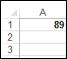
Sub ReferringToASingleCellUsingTheRangeObject()
Range("A1").Value = 89
Range("A1").Font.Bold = True
End Sub
When you press run or F5 on your keyboard, to run your code then you get the following result, in your actual worksheet:
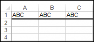
You can use the range object to refer to multiple cells or ranges. For example, if you wanted to refer to cell range (A1:C1) in your VBA code then you could use the VBA range object as shown in the code below:
Sub ReferringToMultipleCellsUsingTheRangeObject()

Range("A1:C1").Value = "ABC"
Range("A1:C1").Borders(xlEdgeBottom).LineStyle = xlDouble

End Sub
When you press run or F5 on your keyboard, to run your code then you get the following result, in your actual worksheet:
Declaring a Variable as a Range
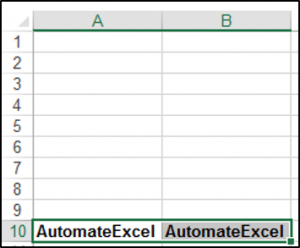
You will need to use the Dim and Set keywords when declaring a variable as a range. The code below shows you how to declare a variable as a range.
Sub DeclaringAndSettingARange()

Dim rng As Range
Set rng = Range("A10:B10")


rng.Value = "AutomateExcel"
rng.Font.Bold = True
rng.Select
rng.Columns.AutoFit

End Sub
The result is:
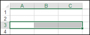
Selecting Specific Rows In Your Range Object
You can select specific rows within your Range Object. The code below shows you how to do this:
Sub SelectingSpecificRowsInTheRangeObject()

Dim rng As Range
Set rng = Range("A1:C3")

rng.Rows(3).Select

End Sub
The result is:
Selecting Specific Columns In Your Range Object
You can select specific columns within your Range Object. The code below shows you how to do this:
Sub SelectingSpecificColumnsInTheRangeObject()

Dim rng As Range
Set rng = Range("A1:C3")

rng.Columns(3).Select

End Sub
VBA Coding Made Easy
Stop searching for VBA code online. Learn more about AutoMacro — A VBA Code Builder that allows beginners to code procedures from scratch with minimal coding knowledge and with many time-saving features for all users!

Learn More!
If you just want to select the used range, use
ActiveSheet.UsedRange.Select
If you want to select from A1 to the end of the used range, you can use the SpecialCells method like this
With ActiveSheet
    .Range(.Cells(1, 1), .Cells.SpecialCells(xlCellTypeLastCell)).Select
End With
Sometimes Excel gets confused on what is the last cell. It’s never a smaller range than the actual used range, but it can be bigger if some cells were deleted. To avoid that, you can use Find and the asterisk wildcard to find the real last cell.
Dim rLastCell As Range

With Sheet1
    Set rLastCell = .Cells.Find("*", .Cells(1, 1), xlValues, xlPart, , xlPrevious)

    .Range(.Cells(1, 1), rLastCell).Select
End With
Finally, make sure you’re only selecting if you really need to. Most of what you need to do in Excel VBA you can do directly to the Range rather than selecting it first. Instead of
.Range(.Cells(1, 1), rLastCell).Select
Selection.Font.Bold = True
You can
.Range(.Cells(1,1), rLastCells).Font.Bold = True
|
5 / 5 / 0 Регистрация: 13.12.2009 Сообщений: 206 |
|
|
1 |
|
Задать диапазон ячеек через переменные17.08.2013, 17:06. Показов 50273. Ответов 1
Привет! такой вопрос: т.е. А100 — плавает. Мне нужно чтобы это число было задано переменной но естественно такое извращение не прокатывает ((
0 |

|
Programming Эксперт 94731 / 64177 / 26122 Регистрация: 12.04.2006 Сообщений: 116,782 |
17.08.2013, 17:06 |
|
1 |
|
Pavel55 971 / 353 / 135 Регистрация: 27.10.2006 Сообщений: 764 |
||||||||
|
17.08.2013, 17:47 |
2 |
|||||||
|
Решение
Ещё можно так Cells (номер_строки, номер_столбца)
4 |
 Сообщение было отмечено Памирыч как решение
Хитрости »
27 Июль 2013 307041 просмотров
Полагаю не совру когда скажу, что все кто программирует в VBA очень часто в своих кодах общаются к ячейкам листов. Ведь это чуть ли не основное предназначение VBA в Excel. В принципе ничего сложного в этом нет. Например, чтобы записать в ячейку A1 слово Привет необходимо выполнить код:
Range("A1").Value = "Привет"
Тоже самое можно сделать сразу для нескольких ячеек:
Range("A1:C10").Value = "Привет"
Если необходимо обратиться к именованному диапазону:
Range("Диапазон1").Select
Диапазон1 — это имя диапазона/ячейки, к которому надо обратиться в коде. Указывается в кавычках, как и адреса ячеек.
Но в VBA есть и альтернативный метод записи значений в ячейке — через объект Cells:
Cells(1, 1).Value = "Привет"
Синтаксис объекта Range:
Range(Cell1, Cell2)
- Cell1 — первая ячейка диапазона. Может быть ссылкой на ячейку или диапазон ячеек, текстовым представлением адреса или имени диапазона/ячейки. Допускается указание несвязанных диапазонов(A1,B10), пересечений(A1 B10).
- Cell2 — последняя ячейка диапазона. Необязательна к указанию. Допускается указание ссылки на ячейку, столбец или строку.
Синтаксис объекта Cells:
Cells(Rowindex, Columnindex)
- Rowindex — номер строки
- Columnindex — номер столбца
Исходя из этого несложно предположить, что к диапазону можно обратиться, используя Cells и Range:
'выделяем диапазон "A1:B10" на активном листе
Range(Cells(1,1), Cells(10,2)).Select
и для чего? Ведь можно гораздо короче:
Иногда обращение посредством Cells куда удобнее. Например для цикла по столбцам(да еще и с шагом 3) совершенно неудобно было бы использовать буквенное обозначение столбцов.
Объект Cells так же можно использовать для указания ячеек внутри непосредственно указанного диапазона. Например, Вам необходимо выделить ячейку в 3 строке и 2 столбце диапазона «D5:F56». Можно пройтись по листу и посмотреть, отсчитать нужное количество строк и столбцов и понять, что это будет «E7». А можно сделать проще:
Range("D5:F56").Cells(3, 2).Select
Согласитесь, это гораздо удобнее, чем отсчитывать каждый раз. Особенно, если придется оперировать смещением не на 2-3 ячейки, а на 20 и более. Конечно, можно было бы применить Offset. Но данное свойство именно смещает диапазон на указанное количество строк и столбцов и придется уменьшать на 1 смещение каждого параметра для получения нужной ячейки. Да и смещает на указанное количество строк и столбцов весь диапазон, а не одну ячейку. Это, конечно, тоже не проблема — можно вдобавок к этому использовать метод Resize — но запись получится несколько длиннее и менее наглядной:
Range("D5:F56").Offset(2, 1).Resize(1, 1).Select
И неплохо бы теперь понять, как значение диапазона присвоить переменной. Для начала переменная должна быть объявлена с типом Range. А т.к. Range относится к глобальному типу Object, то присвоение значения такой переменной должно быть обязательно с применением оператора Set:
Dim rR as Range
Set rR = Range("D5")
если оператор Set не применять, то в лучшем случае получите ошибку, а в худшем(он возможен, если переменной rR не назначать тип) переменной будет назначено значение Null или значение ячейки по умолчанию. Почему это хуже? Потому что в таком случае код продолжит выполняться, но логика кода будет неверной, т.к. эта самая переменная будет содержать значение неверного типа и применение её в коде в дальнейшем все равно приведет к ошибке. Только ошибку эту отловить будет уже сложнее.
Использовать же такую переменную в дальнейшем можно так же, как и прямое обращение к диапазону:
Вроде бы на этом можно было завершить, но…Это как раз только начало. То, что я написал выше знает практически каждый, кто пишет в VBA. Основной же целью этой статьи было пояснить некоторые нюансы обращения к диапазонам. Итак, поехали.
Обычно макрорекордер при обращении к диапазону(да и любым другим объектам) сначала его выделяет, а потом уже изменяет свойство или вызывает некий метод:
'так выглядит запись слова Test в ячейку А1
Range("A1").Select
Selection.Value = "Test"
Но как правило выделение — действие лишнее. Можно записать значение и без него:
'запишем слово Test в ячейку A1 на активном листе
Range("A1").Value = "Test"
Теперь чуть подробнее разберем, как обратиться к диапазону не выделяя его и при этом сделать все правильно. Диапазон и ячейка — это объекты листа. У каждого объекта есть родитель — грубо говоря это другой объект, который является управляющим для дочернего объекта. Для ячейки родительский объект — Лист, для Листа — Книга, для Книги — Приложение Excel. Если смотреть на иерархию зависимости объектов, то от старшего к младшему получится так:
Applicaton => Workbooks => Sheets => Range
По умолчанию для всех диапазонов и ячеек родительским объектом является текущий(активный) лист. Т.е. если для диапазона(ячейки) не указать явно лист, к которому он относится, в качестве родительского листа для него будет использован текущий — ActiveSheet:
'запишем слово Test в ячейку A1 на активном листе
Range("A1").Value = "Test"
Т.е. если в данный момент активен Лист1 — то слово Test будет записано в ячейку А1 Лист1. Если активен Лист3 — в А1 Лист3. Иначе говоря такая запись равносильна записи:
ActiveSheet.Range("A1").Value = "Test"
Поэтому выхода два — либо активировать сначала нужный лист, либо записать без активации.
'активируем Лист2
Worksheets("Лист2").Select
'записываем слово Test в ячейку A1
Range("A1").Value = "Test"
Чтобы не активируя другой лист записать в него данные, необходимо явно указать принадлежность объекта Range именно этому листу:
'запишем слово Test в ячейку A1 на Лист2 независимо от того, какой лист активен
Worksheets("Лист2").Range("A1").Value = "Test"
Таким же образом происходит считывание данных с ячеек — если не указывать лист, данные ячеек которого необходимо считать — считаны будут данные с ячейки активного листа. Чтобы считать данные с Лист2 независимо от того, какой лист активен применяется такой код:
'считываем значение ячейки A1 с Лист2 независимо от того, какой лист активен
MsgBox Worksheets("Лист2").Range("A1").Value
Т.к. ячейка является частью листа, то лист в свою очередь является частью книги. Исходя из того легко сделать вывод, что при открытых двух и более книгах мы так же можем обратиться к ячейкам любого листа любой открытой книги не активируя при этом ни книгу, ни лист:
'запишем слово Test в ячейку A1 на Лист2 книги Книга2.xlsx независимо от того, какая книга и какой лист активен
Workbooks("Книга2.xlsx").Worksheets("Лист2").Range("A1").Value = "Test"
'считываем значение ячейки A1 с Лист2 книги Книга3.xlsx независимо от того, какой лист активен
MsgBox Workbooks("Книга3.xlsx").Worksheets("Лист2").Range("A1").Value
Важный момент: лучше всегда указать имя книги вместе с расширением(.xlsx, xlsm, .xls и т.д.). Если в настройках ОС Windows(Панель управления —Параметры папок -вкладка Вид —Скрывать расширения для зарегистрированных типов файлов) указано скрывать расширения — то указывать расширение не обязательно — Workbooks(«Книга2»). Но и ошибки не будет, если его указать. Однако, если пункт «Скрывать расширения для зарегистрированных типов файлов» отключен, то указание Workbooks(«Книга2») обязательно приведет к ошибке.
Очень часто ошибки обращения к ячейкам листов и книг делают начинающие, особенно в циклах по листам. Вот пример неправильного цикла:
Dim wsSh As Worksheet
For Each wsSh In ActiveWorkbook.Worksheets
    Range("A1").Value = wsSh.Name 'записываем в ячейку А1 имя листа
    MsgBox Range("A1").Value 'проверяем, то ли имя записалось
Next wsSh
MsgBox будет выдавать правильные значения, но сами имена листов будут записываться не на каждый лист, а последовательно в ячейку активного листа. Поэтому на активном листе в ячейке А1 будет имя последнего листа.
А вот так выглядит правильный цикл:
Вариант 1 — активация листа(медленный)
Dim wsSh As Worksheet
For Each wsSh In ActiveWorkbook.Worksheets
    wsSh.Activate 'активируем каждый лист
    Range("A1").Value = wsSh.Name 'записываем в ячейку А1 имя листа
    MsgBox Range("A1").Value 'проверяем, то ли имя записалось
Next wsSh
Вариант 2 — без активации листа(быстрый и более правильный)
Dim wsSh As Worksheet
For Each wsSh In ActiveWorkbook.Worksheets
    wsSh.Range("A1").Value = wsSh.Name 'записываем в ячейку А1 имя листа
    MsgBox wsSh.Range("A1").Value 'проверяем, то ли имя записалось
Next wsSh
Важно: если код записан в модуле листа(правая кнопка мыши на листе-Исходный текст) и для объекта Range или Cells родитель явно не указан(т.е. нет имени листа и книги) — тогда в качестве родителя будет использован именно тот лист, в котором записан код, независимо от того какой лист активный. Иными словами — если в модуле листа записать обращение вроде Range(«A1»).Value = «привет», то слово привет всегда будет записывать в ячейку A1 именно того листа, в котором записан сам код. Это следует учитывать, когда располагаете свои коды внутри модулей листов.
В конструкциях типа Range(Cells(,),Cells(,)) Range является контейнером, в котором указываются ссылки на объекты, из которых и будет создана ссылка на непосредственно конечный объект.
Предположим, что активен «Лист1», а код запущен с листа «Итог».
Если запись будет вида
Sheets("Итог").Range(Cells(1, 1), Cells(10, 1))
это вызовет ошибку «Run-time error ‘1004’: Application-defined or object-defined error». А ошибка появляется потому, что контейнер и объекты внутри него не могут располагаться на разных листах, равно как и:
Sheets("Итог").Range(Cells(1, 1), Sheets("Итог").Cells(10, 1))
'запись ниже так же неверна
Range(Cells(1, 1), Sheets("Итог").Cells(10, 1))
т.к. ссылки на объекты внутри контейнера относятся к разным листам. Cells(1, 1) — к активному листу, а Sheets(«Итог»).Cells(10, 1) — к листу Итог.
А вот такие записи будут правильными:
Sheets("Итог").Range(Sheets("Итог").Cells(1, 1), Sheets("Итог").Cells(10, 1))
Range(Sheets("Итог").Cells(1, 1), Sheets("Итог").Cells(10, 1))
Вторая запись не содержит ссылки на родителя для Range, но ошибки это в большинстве случаев не вызовет — т.к. если для контейнера ссылка не указана, а для двух объектов внутри контейнера родитель один — он будет применен и для самого контейнера. Однако лучше делать как в первой строке — т.е. с обязательным указанием родителя для контейнера и для его составляющих. Т.к. при определенных обстоятельствах(например, если в момент обращения к диапазону активной является книга, открытая в режиме защищенного просмотра) обращение к Range без родителя может вызывать ошибку выполнения.
Если запись будет вида Range(«A1″,»A10»), то указывать ссылку на родителя внутри Range не обязательно — достаточно будет указать эту ссылку перед самим Range — Sheets(«Итог»).Range(«A1″,»A10»), т.к. текстовое представление адреса внутри Range не является объектом(у которого может быть какой-то родительский объект), что обязывает создать ссылку именно на родителя контейнера.
Разберем пример, приближенный к жизненной ситуации. Необходимо на лист Итог занести формулу вычитания, начиная с ячейки А2 и до последней заполненной. На момент записи активен Лист1. Очень часто начинающие записывают так:
Sheets("Итог").Range("A2:A" & Cells(Rows.Count, 1).End(xlUp).Row) _
                                        .FormulaR1C1 = "=RC2-RC11"
Запись смешанная — и текстовое представление адреса ячейки(«A2:A») и ссылка на объект Cells. В данном случае явную ошибку код не вызовет, но и работать будет не всегда так, как хотелось бы. А это самое плохое, что может случиться при разработке.
Sheets(«Итог»).Range(«A2:A» — создается ссылка на столбец "A" листа Итог. Но далее идет вычисление последней строки первого столбца. И вот как раз это вычисление происходит на основе объекта Cells, который не содержит в себе ссылки на родительский объект. А значит он будет вычислять последнюю строку исключительно для текущего листа(если код записан в стандартном модуле, а не модуле листа) — т.е. для Лист1. Правильно было бы записать так:
Sheets("Итог").Range("A2:A" & Sheets("Итог").Cells(Rows.Count, 1).End(xlUp).Row) _
                                                      .FormulaR1C1 = "=RC2-RC11"
Но и здесь неверное обращение с диапазоном может сыграть злую шутку. Например, надо получить последнюю заполненную ячейку в конкретной книге:
lLastRow = Workbooks("Книга3.xls").Sheets("Лист1").Cells(Rows.Count, 1).End(xlUp).Row
с виду все нормально, но есть нюанс. Rows.Count по умолчанию будет относится к активной книге, если записано в стандартном модуле. Приведенный выше код должен работать с книгой формата 97-2003 и вычислить последнюю заполненную ячейку на листе1. В книгах формата Excel 97-2003(.xls) всего 65536 строк. Если в момент выполнения приведенной строки активна книга формата 2007 и выше(форматы .xlsx, .xlsm, .xlsb и пр) — то Rows.Count вернет 1048576, т.к. именно такое количество строк в листах книг версий Excel, начиная с 2007. И т.к. в книге, в которой мы пытаемся вычислить последнюю строку всего 65536 строк — получим ошибку 1004, т.к. не может быть номера строки 1048576 на листе с количеством строк 65536. Поэтому имеет смысл указывать явно откуда считывать Rows.Count:
lLastRow = Workbooks("Книга3.xls").Sheets("Лист1").Cells(Workbooks("Книга3.xls").Sheets("Лист1").Rows.Count, 1).End(xlUp).Row
или применить конструкцию With
With Workbooks("Книга3.xls").Sheets("Лист1")
    lLastRow = .Cells(.Rows.Count, 1).End(xlUp).Row
End With
Также не мешало бы упомянуть возможность выделения несмежного диапазона(часто его называют «рваным»). Это диапазон, который обычно привыкли выделять на листе при помощи зажатой клавиши Ctrl. Что это дает? Это дает возможность выделить одновременно ячейки A1 и B10 и записать значения только в них. Для этого есть несколько способов. Самый очевидный и описанный в справке — метод Union:
Union(Range("A1"), Range("B10")).Value = "Привет"
Однако существует и другой метод:
Range("A1,B10").Value = "Привет"
В чем отличие(я бы даже сказал преимущество) Union: можно применять в цикле по условию. Например, выделить в диапазоне A1:F50 только те ячейки, значение которых больше 10 и меньше 20:
Sub SelOne()
    Dim rCell As Range, rSel As Range
    For Each rCell In Range("A1:F50")
        If rCell.Value > 10 And rCell.Value < 20 Then
            If rSel Is Nothing Then
                Set rSel = rCell
            Else
                Set rSel = Union(rSel, rCell)
            End If
        End If
    Next rCell
    If Not rSel Is Nothing Then rSel.Select
End Sub
Конечно, можно и просто в Range через запятую передать все эти ячейки, сформировав предварительно строку. Но в случае со строкой действует ограничение: длина строки не должна превышать 255 символов.
Надеюсь, что после прочтения данной статьи проблем с обращением к диапазонам и ячейкам у Вас будет гораздо меньше.
Также см.:
Как определить последнюю ячейку на листе через VBA?
Как определить первую заполненную ячейку на листе?
Как из Excel обратиться к другому приложению
Статья помогла? Поделись ссылкой с друзьями!
![]() Видеоуроки
Видеоуроки
Поиск по меткам
Access
apple watch
Multex
Power Query и Power BI
VBA управление кодами
Бесплатные надстройки
Дата и время
Записки
ИП
Надстройки
Печать
Политика Конфиденциальности
Почта
Программы
Работа с приложениями
Разработка приложений
Росстат
Тренинги и вебинары
Финансовые
Форматирование
Функции Excel
акции MulTEx
ссылки
статистика
“It is a capital mistake to theorize before one has data”- Sir Arthur Conan Doyle
This post covers everything you need to know about using Cells and Ranges in VBA. You can read it from start to finish as it is laid out in a logical order. If you prefer you can use the table of contents below to go to a section of your choice.
Topics covered include Offset property, reading values between cells, reading values to arrays and formatting cells.
A Quick Guide to Ranges and Cells
| Function | Takes | Returns | Example | Gives |
|---|---|---|---|---|
|
Range |
cell address | multiple cells | .Range(«A1:A4») | $A$1:$A$4 |
| Cells | row, column | one cell | .Cells(1,5) | $E$1 |
| Offset | row, column | multiple cells | Range(«A1:A2») .Offset(1,2) |
$C$2:$C$3 |
| Rows | row(s) | one or more rows | .Rows(4) .Rows(«2:4») |
$4:$4 $2:$4 |
| Columns | column(s) | one or more columns | .Columns(4) .Columns(«B:D») |
$D:$D $B:$D |
Download the Code
The Webinar
If you are a member of the VBA Vault, then click on the image below to access the webinar and the associated source code.
(Note: Website members have access to the full webinar archive.)

Introduction
This is the third post dealing with the three main elements of VBA. These three elements are the Workbooks, Worksheets and Ranges/Cells. Cells are by far the most important part of Excel. Almost everything you do in Excel starts and ends with Cells.
Generally speaking, you do three main things with Cells
- Read from a cell.
- Write to a cell.
- Change the format of a cell.
Excel has a number of methods for accessing cells such as Range, Cells and Offset.These can cause confusion as they do similar things and can lead to confusion
In this post I will tackle each one, explain why you need it and when you should use it.
Let’s start with the simplest method of accessing cells – using the Range property of the worksheet.
Important Notes
I have recently updated this article so that is uses Value2.
You may be wondering what is the difference between Value, Value2 and the default:
' Value2
Range("A1").Value2 = 56

' Value
Range("A1").Value = 56

' Default uses value
Range("A1") = 56
Using Value may truncate number if the cell is formatted as currency. If you don’t use any property then the default is Value.
It is better to use Value2 as it will always return the actual cell value(see this article from Charle Williams.)
The Range Property
The worksheet has a Range property which you can use to access cells in VBA. The Range property takes the same argument that most Excel Worksheet functions take e.g. “A1”, “A3:C6” etc.
The following example shows you how to place a value in a cell using the Range property.
' https://excelmacromastery.com/
Public Sub WriteToCell()

    ' Write number to cell A1 in sheet1 of this workbook
    ThisWorkbook.Worksheets("Sheet1").Range("A1").Value2 = 67

    ' Write text to cell A2 in sheet1 of this workbook
    ThisWorkbook.Worksheets("Sheet1").Range("A2").Value2 = "John Smith"

    ' Write date to cell A3 in sheet1 of this workbook
    ThisWorkbook.Worksheets("Sheet1").Range("A3").Value2 = #11/21/2017#

End Sub
As you can see Range is a member of the worksheet which in turn is a member of the Workbook. This follows the same hierarchy as in Excel so should be easy to understand. To do something with Range you must first specify the workbook and worksheet it belongs to.
For the rest of this post I will use the code name to reference the worksheet.

The following code shows the above example using the code name of the worksheet i.e. Sheet1 instead of ThisWorkbook.Worksheets(“Sheet1”).
' https://excelmacromastery.com/
Public Sub UsingCodeName()

    ' Write number to cell A1 in sheet1 of this workbook
    Sheet1.Range("A1").Value2 = 67

    ' Write text to cell A2 in sheet1 of this workbook
    Sheet1.Range("A2").Value2 = "John Smith"

    ' Write date to cell A3 in sheet1 of this workbook
    Sheet1.Range("A3").Value2 = #11/21/2017#

End Sub
You can also write to multiple cells using the Range property
' https://excelmacromastery.com/
Public Sub WriteToMulti()

    ' Write number to a range of cells
    Sheet1.Range("A1:A10").Value2 = 67

    ' Write text to multiple ranges of cells
    Sheet1.Range("B2:B5,B7:B9").Value2 = "John Smith"

End Sub
You can download working examples of all the code from this post from the top of this article.
The Cells Property of the Worksheet
The worksheet object has another property called Cells which is very similar to range. There are two differences
- Cells returns a range of one cell only.
- Cells takes row and column as arguments.
The example below shows you how to write values to cells using both the Range and Cells property
' https://excelmacromastery.com/
Public Sub UsingCells()

    ' Write to A1
    Sheet1.Range("A1").Value2 = 10
    Sheet1.Cells(1, 1).Value2  = 10

    ' Write to A10
    Sheet1.Range("A10").Value2 = 10
    Sheet1.Cells(10, 1).Value2  = 10

    ' Write to E1
    Sheet1.Range("E1").Value2 = 10
    Sheet1.Cells(1, 5).Value2  = 10

End Sub
You may be wondering when you should use Cells and when you should use Range. Using Range is useful for accessing the same cells each time the Macro runs.
For example, if you were using a Macro to calculate a total and write it to cell A10 every time then Range would be suitable for this task.
Using the Cells property is useful if you are accessing a cell based on a number that may vary. It is easier to explain this with an example.
In the following code, we ask the user to specify the column number. Using Cells gives us the flexibility to use a variable number for the column.
' https://excelmacromastery.com/
Public Sub WriteToColumn()

    Dim UserCol As Integer

    ' Get the column number from the user
    UserCol = Application.InputBox(" Please enter the column...", Type:=1)

    ' Write text to user selected column
    Sheet1.Cells(1, UserCol).Value2 = "John Smith"

End Sub
In the above example, we are using a number for the column rather than a letter.
To use Range here would require us to convert these values to the letter/number cell reference e.g. “C1”. Using the Cells property allows us to provide a row and a column number to access a cell.
Sometimes you may want to return more than one cell using row and column numbers. The next section shows you how to do this.
Using Cells and Range together
As you have seen you can only access one cell using the Cells property. If you want to return a range of cells then you can use Cells with Ranges as follows
' https://excelmacromastery.com/
Public Sub UsingCellsWithRange()

    With Sheet1
        ' Write 5 to Range A1:A10 using Cells property
        .Range(.Cells(1, 1), .Cells(10, 1)).Value2 = 5

        ' Format Range B1:Z1 to be bold
        .Range(.Cells(1, 2), .Cells(1, 26)).Font.Bold = True

    End With

End Sub
As you can see, you provide the start and end cell of the Range. Sometimes it can be tricky to see which range you are dealing with when the value are all numbers. Range has a property called Address which displays the letter/ number cell reference of any range. This can come in very handy when you are debugging or writing code for the first time.
In the following example we print out the address of the ranges we are using:
' https://excelmacromastery.com/
Public Sub ShowRangeAddress()

    ' Note: Using underscore allows you to split up lines of code
    With Sheet1

        ' Write 5 to Range A1:A10 using Cells property
        .Range(.Cells(1, 1), .Cells(10, 1)).Value2 = 5
        Debug.Print "First address is : " _
            + .Range(.Cells(1, 1), .Cells(10, 1)).Address

        ' Format Range B1:Z1 to be bold
        .Range(.Cells(1, 2), .Cells(1, 26)).Font.Bold = True
        Debug.Print "Second address is : " _
            + .Range(.Cells(1, 2), .Cells(1, 26)).Address

    End With

End Sub
In the example I used Debug.Print to print to the Immediate Window. To view this window select View->Immediate Window(or Ctrl G)


You can download all the code for this post from the top of this article.
The Offset Property of Range
Range has a property called Offset. The term Offset refers to a count from the original position. It is used a lot in certain areas of programming. With the Offset property you can get a Range of cells the same size and a certain distance from the current range. The reason this is useful is that sometimes you may want to select a Range based on a certain condition. For example in the screenshot below there is a column for each day of the week. Given the day number(i.e. Monday=1, Tuesday=2 etc.) we need to write the value to the correct column.

We will first attempt to do this without using Offset.
' https://excelmacromastery.com/
' This sub tests with different values
Public Sub TestSelect()

    ' Monday
    SetValueSelect 1, 111.21
    ' Wednesday
    SetValueSelect 3, 456.99
    ' Friday
    SetValueSelect 5, 432.25
    ' Sunday
    SetValueSelect 7, 710.17

End Sub

' Writes the value to a column based on the day
Public Sub SetValueSelect(lDay As Long, lValue As Currency)

    Select Case lDay
        Case 1: Sheet1.Range("H3").Value2 = lValue
        Case 2: Sheet1.Range("I3").Value2 = lValue
        Case 3: Sheet1.Range("J3").Value2 = lValue
        Case 4: Sheet1.Range("K3").Value2 = lValue
        Case 5: Sheet1.Range("L3").Value2 = lValue
        Case 6: Sheet1.Range("M3").Value2 = lValue
        Case 7: Sheet1.Range("N3").Value2 = lValue
    End Select

End Sub
As you can see in the example, we need to add a line for each possible option. This is not an ideal situation. Using the Offset Property provides a much cleaner solution
' https://excelmacromastery.com/
' This sub tests with different values
Public Sub TestOffset()

    DayOffSet 1, 111.01
    DayOffSet 3, 456.99
    DayOffSet 5, 432.25
    DayOffSet 7, 710.17

End Sub

Public Sub DayOffSet(lDay As Long, lValue As Currency)

    ' We use the day value with offset specify the correct column
    Sheet1.Range("G3").Offset(, lDay).Value2 = lValue

End Sub
As you can see this solution is much better. If the number of days in increased then we do not need to add any more code. For Offset to be useful there needs to be some kind of relationship between the positions of the cells. If the Day columns in the above example were random then we could not use Offset. We would have to use the first solution.
One thing to keep in mind is that Offset retains the size of the range. So .Range(“A1:A3”).Offset(1,1) returns the range B2:B4. Below are some more examples of using Offset
' https://excelmacromastery.com/
Public Sub UsingOffset()

    ' Write to B2 - no offset
    Sheet1.Range("B2").Offset().Value2 = "Cell B2"

    ' Write to C2 - 1 column to the right
    Sheet1.Range("B2").Offset(, 1).Value2 = "Cell C2"

    ' Write to B3 - 1 row down
    Sheet1.Range("B2").Offset(1).Value2 = "Cell B3"

    ' Write to C3 - 1 column right and 1 row down
    Sheet1.Range("B2").Offset(1, 1).Value2 = "Cell C3"

    ' Write to A1 - 1 column left and 1 row up
    Sheet1.Range("B2").Offset(-1, -1).Value2 = "Cell A1"

    ' Write to range E3:G13 - 1 column right and 1 row down
    Sheet1.Range("D2:F12").Offset(1, 1).Value2 = "Cells E3:G13"

End Sub
Using the Range CurrentRegion
CurrentRegion returns a range of all the adjacent cells to the given range.
In the screenshot below you can see the two current regions. I have added borders to make the current regions clear.

A row or column of blank cells signifies the end of a current region.
You can manually check the CurrentRegion in Excel by selecting a range and pressing Ctrl + Shift + *.
If we take any range of cells within the border and apply CurrentRegion, we will get back the range of cells in the entire area.
For example
Range(“B3”).CurrentRegion will return the range B3:D14
Range(“D14”).CurrentRegion will return the range B3:D14
Range(“C8:C9”).CurrentRegion will return the range B3:D14
and so on
How to Use
We get the CurrentRegion as follows
' Current region will return B3:D14 from above example
Dim rg As Range
Set rg = Sheet1.Range("B3").CurrentRegion
Read Data Rows Only
Read through the range from the second row i.e.skipping the header row
' Current region will return B3:D14 from above example
Dim rg As Range
Set rg = Sheet1.Range("B3").CurrentRegion

' Start at row 2 - row after header
Dim i As Long
For i = 2 To rg.Rows.Count
    ' current row, column 1 of range
    Debug.Print rg.Cells(i, 1).Value2
Next i
Remove Header
Remove header row(i.e. first row) from the range. For example if range is A1:D4 this will return A2:D4
' Current region will return B3:D14 from above example
Dim rg As Range
Set rg = Sheet1.Range("B3").CurrentRegion

' Remove Header
Set rg = rg.Resize(rg.Rows.Count - 1).Offset(1)

' Start at row 1 as no header row
Dim i As Long
For i = 1 To rg.Rows.Count
    ' current row, column 1 of range
    Debug.Print rg.Cells(i, 1).Value2
Next i
Using Rows and Columns as Ranges
If you want to do something with an entire Row or Column you can use the Rows or Columns property of the Worksheet. They both take one parameter which is the row or column number you wish to access
' https://excelmacromastery.com/
Public Sub UseRowAndColumns()

    ' Set the font size of column B to 9
    Sheet1.Columns(2).Font.Size = 9

    ' Set the width of columns D to F
    Sheet1.Columns("D:F").ColumnWidth = 4

    ' Set the font size of row 5 to 18
    Sheet1.Rows(5).Font.Size = 18

End Sub
Using Range in place of Worksheet
You can also use Cells, Rows and Columns as part of a Range rather than part of a Worksheet. You may have a specific need to do this but otherwise I would avoid the practice. It makes the code more complex. Simple code is your friend. It reduces the possibility of errors.
The code below will set the second column of the range to bold. As the range has only two rows the entire column is considered B1:B2
' https://excelmacromastery.com/
Public Sub UseColumnsInRange()

    ' This will set B1 and B2 to be bold
    Sheet1.Range("A1:C2").Columns(2).Font.Bold = True

End Sub
You can download all the code for this post from the top of this article.
Reading Values from one Cell to another
In most of the examples so far we have written values to a cell. We do this by placing the range on the left of the equals sign and the value to place in the cell on the right. To write data from one cell to another we do the same. The destination range goes on the left and the source range goes on the right.
The following example shows you how to do this:
' https://excelmacromastery.com/
Public Sub ReadValues()

    ' Place value from B1 in A1
    Sheet1.Range("A1").Value2 = Sheet1.Range("B1").Value2

    ' Place value from B3 in sheet2 to cell A1
    Sheet1.Range("A1").Value2 = Sheet2.Range("B3").Value2

    ' Place value from B1 in cells A1 to A5
    Sheet1.Range("A1:A5").Value2 = Sheet1.Range("B1").Value2

    ' You need to use the "Value" property to read multiple cells
    Sheet1.Range("A1:A5").Value2 = Sheet1.Range("B1:B5").Value2

End Sub
As you can see from this example it is not possible to read from multiple cells. If you want to do this you can use the Copy function of Range with the Destination parameter
' https://excelmacromastery.com/
Public Sub CopyValues()

    ' Store the copy range in a variable
    Dim rgCopy As Range
    Set rgCopy = Sheet1.Range("B1:B5")

    ' Use this to copy from more than one cell
    rgCopy.Copy Destination:=Sheet1.Range("A1:A5")

    ' You can paste to multiple destinations
    rgCopy.Copy Destination:=Sheet1.Range("A1:A5,C2:C6")

End Sub
The Copy function copies everything including the format of the cells. It is the same result as manually copying and pasting a selection. You can see more about it in the Copying and Pasting Cells section.
Using the Range.Resize Method
When copying from one range to another using assignment(i.e. the equals sign), the destination range must be the same size as the source range.
Using the Resize function allows us to resize a range to a given number of rows and columns.
For example:
' https://excelmacromastery.com/
Sub ResizeExamples()

    ' Prints A1
    Debug.Print Sheet1.Range("A1").Address

    ' Prints A1:A2
    Debug.Print Sheet1.Range("A1").Resize(2, 1).Address

    ' Prints A1:A5
    Debug.Print Sheet1.Range("A1").Resize(5, 1).Address

    ' Prints A1:D1
    Debug.Print Sheet1.Range("A1").Resize(1, 4).Address

    ' Prints A1:C3
    Debug.Print Sheet1.Range("A1").Resize(3, 3).Address

End Sub
When we want to resize our destination range we can simply use the source range size.
In other words, we use the row and column count of the source range as the parameters for resizing:
' https://excelmacromastery.com/
Sub Resize()

    Dim rgSrc As Range, rgDest As Range

    ' Get all the data in the current region
    Set rgSrc = Sheet1.Range("A1").CurrentRegion

      ' Get the range destination
    Set rgDest = Sheet2.Range("A1")
    Set rgDest = rgDest.Resize(rgSrc.Rows.Count, rgSrc.Columns.Count)

    rgDest.Value2 = rgSrc.Value2

End Sub
We can do the resize in one line if we prefer:
' https://excelmacromastery.com/
Sub ResizeOneLine()

    Dim rgSrc As Range

    ' Get all the data in the current region
    Set rgSrc = Sheet1.Range("A1").CurrentRegion

    With rgSrc
        Sheet2.Range("A1").Resize(.Rows.Count, .Columns.Count).Value2 = .Value2
    End With

End Sub
Reading Values to variables
We looked at how to read from one cell to another. You can also read from a cell to a variable. A variable is used to store values while a Macro is running. You normally do this when you want to manipulate the data before writing it somewhere. The following is a simple example using a variable. As you can see the value of the item to the right of the equals is written to the item to the left of the equals.
' https://excelmacromastery.com/
Public Sub UseVariables()

    ' Create
    Dim number As Long

    ' Read number from cell
    number = Sheet1.Range("A1").Value2

    ' Add 1 to value
    number = number + 1

    ' Write new value to cell
    Sheet1.Range("A2").Value2 = number

End Sub
To read text to a variable you use a variable of type String:
' https://excelmacromastery.com/
Public Sub UseVariableText()

    ' Declare a variable of type string
    Dim text As String

    ' Read value from cell
    text = Sheet1.Range("A1").Value2

    ' Write value to cell
    Sheet1.Range("A2").Value2 = text

End Sub
You can write a variable to a range of cells. You just specify the range on the left and the value will be written to all cells in the range.
' https://excelmacromastery.com/
Public Sub VarToMulti()

    ' Read value from cell
    Sheet1.Range("A1:B10").Value2 = 66

End Sub
You cannot read from multiple cells to a variable. However you can read to an array which is a collection of variables. We will look at doing this in the next section.
How to Copy and Paste Cells
If you want to copy and paste a range of cells then you do not need to select them. This is a common error made by new VBA users.
Note: We normally use Range.Copy when we want to copy formats, formulas, validation. If we want to copy values it is not the most efficient method.
I have written a complete guide to copying data in Excel VBA here.
You can simply copy a range of cells like this:
Range("A1:B4").Copy Destination:=Range("C5")
Using this method copies everything – values, formats, formulas and so on. If you want to copy individual items you can use the PasteSpecial property of range.
It works like this
Range("A1:B4").Copy
Range("F3").PasteSpecial Paste:=xlPasteValues
Range("F3").PasteSpecial Paste:=xlPasteFormats
Range("F3").PasteSpecial Paste:=xlPasteFormulas
The following table shows a full list of all the paste types
| Paste Type |
|---|
| xlPasteAll |
| xlPasteAllExceptBorders |
| xlPasteAllMergingConditionalFormats |
| xlPasteAllUsingSourceTheme |
| xlPasteColumnWidths |
| xlPasteComments |
| xlPasteFormats |
| xlPasteFormulas |
| xlPasteFormulasAndNumberFormats |
| xlPasteValidation |
| xlPasteValues |
| xlPasteValuesAndNumberFormats |
Reading a Range of Cells to an Array
You can also copy values by assigning the value of one range to another.
Range("A3:Z3").Value2 = Range("A1:Z1").Value2
The value of range in this example is considered to be a variant array. What this means is that you can easily read from a range of cells to an array. You can also write from an array to a range of cells. If you are not familiar with arrays you can check them out in this post.
The following code shows an example of using an array with a range:
' https://excelmacromastery.com/
Public Sub ReadToArray()

    ' Create dynamic array
    Dim StudentMarks() As Variant

    ' Read 26 values into array from the first row
    StudentMarks = Range("A1:Z1").Value2

    ' Do something with array here

    ' Write the 26 values to the third row
    Range("A3:Z3").Value2 = StudentMarks

End Sub
Keep in mind that the array created by the read is a 2 dimensional array. This is because a spreadsheet stores values in two dimensions i.e. rows and columns
Going through all the cells in a Range
Sometimes you may want to go through each cell one at a time to check value.
You can do this using a For Each loop shown in the following code
' https://excelmacromastery.com/
Public Sub TraversingCells()

    ' Go through each cells in the range
    Dim rg As Range
    For Each rg In Sheet1.Range("A1:A10,A20")
        ' Print address of cells that are negative
        If rg.Value < 0 Then
            Debug.Print rg.Address + " is negative."
        End If
    Next

End Sub
You can also go through consecutive Cells using the Cells property and a standard For loop.
The standard loop is more flexible about the order you use but it is slower than a For Each loop.
' https://excelmacromastery.com/
Public Sub TraverseCells()

    ' Go through cells from A1 to A10
    Dim i As Long
    For i = 1 To 10
        ' Print address of cells that are negative
        If Range("A" & i).Value < 0 Then
            Debug.Print Range("A" & i).Address + " is negative."
        End If
    Next

    ' Go through cells in reverse i.e. from A10 to A1
    For i = 10 To 1 Step -1
        ' Print address of cells that are negative
        If Range("A" & i) < 0 Then
            Debug.Print Range("A" & i).Address + " is negative."
        End If
    Next

End Sub
Formatting Cells
Sometimes you will need to format the cells the in spreadsheet. This is actually very straightforward. The following example shows you various formatting you can add to any range of cells
' https://excelmacromastery.com/
Public Sub FormattingCells()

    With Sheet1

        ' Format the font
        .Range("A1").Font.Bold = True
        .Range("A1").Font.Underline = True
        .Range("A1").Font.Color = rgbNavy

        ' Set the number format to 2 decimal places
        .Range("B2").NumberFormat = "0.00"
        ' Set the number format to a date
        .Range("C2").NumberFormat = "dd/mm/yyyy"
        ' Set the number format to general
        .Range("C3").NumberFormat = "General"
        ' Set the number format to text
        .Range("C4").NumberFormat = "Text"

        ' Set the fill color of the cell
        .Range("B3").Interior.Color = rgbSandyBrown

        ' Format the borders
        .Range("B4").Borders.LineStyle = xlDash
        .Range("B4").Borders.Color = rgbBlueViolet

    End With

End Sub
Main Points
The following is a summary of the main points
- Range returns a range of cells
- Cells returns one cells only
- You can read from one cell to another
- You can read from a range of cells to another range of cells.
- You can read values from cells to variables and vice versa.
- You can read values from ranges to arrays and vice versa
- You can use a For Each or For loop to run through every cell in a range.
- The properties Rows and Columns allow you to access a range of cells of these types
What’s Next?
Free VBA Tutorial If you are new to VBA or you want to sharpen your existing VBA skills then why not try out the The Ultimate VBA Tutorial.
Related Training: Get full access to the Excel VBA training webinars and all the tutorials.
(NOTE: Planning to build or manage a VBA Application? Learn how to build 10 Excel VBA applications from scratch.)
# Ways to refer to a single cell
The simplest way to refer to a single cell on the current Excel worksheet is simply to enclose the A1 form of its reference in square brackets:
Note that square brackets are just convenient syntactic sugar (opens new window) for the Evaluate method of the Application object, so technically, this is identical to the following code:
You could also call the Cells method which takes a row and a column and returns a cell reference.
Remember that whenever you pass a row and a column to Excel from VBA, the row is always first, followed by the column, which is confusing because it is the opposite of the common A1 notation where the column appears first.
In both of these examples, we did not specify a worksheet, so Excel will use the active sheet (the sheet that is in front in the user interface). You can specify the active sheet explicitly:
Or you can provide the name of a particular sheet:
There are a wide variety of methods that can be used to get from one range to another. For example, the Rows method can be used to get to the individual rows of any range, and the Cells method can be used to get to individual cells of a row or column, so the following code refers to cell C1:
# Creating a Range
A Range (opens new window) cannot be created or populated the same way a string would:
It is considered best practice to qualify your references (opens new window), so from now on we will use the same approach here.
More about Creating Object Variables (e.g. Range) on MSDN (opens new window) . More about Set Statement on MSDN (opens new window).
There are different ways to create the same Range:
Note in the example that Cells(2, 1) is equivalent to Range(«A2»). This is because Cells returns a Range object.
Some sources: Chip Pearson-Cells Within Ranges (opens new window); MSDN-Range Object (opens new window); John Walkenback-Referring To Ranges In Your VBA Code (opens new window).
Also note that in any instance where a number is used in the declaration of the range, and the number itself is outside of quotation marks, such as Range(«A» & 2), you can swap that number for a variable that contains an integer/long. For example:
If you are using double loops, Cells is better:
# Offset Property
- Offset(Rows, Columns) — The operator used to statically reference another point from the current cell. Often used in loops. It should be understood that positive numbers in the rows section moves right, wheres as negatives move left. With the columns section positives move down and negatives move up.
i.e
This code selects B2, puts a new string there, then moves that string back to A1 afterwards clearing out B2.
# Saving a reference to a cell in a variable
To save a reference to a cell in a variable, you must use the Set syntax, for example:
later…
Why is the Set keyword required? Set tells Visual Basic that the value on the right hand side of the = is meant to be an object.
# How to Transpose Ranges (Horizontal to Vertical & vice versa)
Note: Copy/PasteSpecial also has a Paste Transpose option which updates the transposed cells’ formulas as well.
# Syntax
- Set — The operator used to set a reference to an object, such as a Range
- For Each — The operator used to loop through every item in a collection
Note that the variable names r, cell and others can be named however you like but should be named appropriately so the code is easier to understand for you and others.
Excel VBA Variable Range
In this article, we will see an outline on Excel VBA Variable in Range. But using a range property means a user has to know which range to use that’s where range as variable comes in. In VBA we have a data type as a range that is used to define variables as a range that can hold a value of the range. These variables are very useful in complex programming and automation. Often variable range is used with the set statements and range method. Set statements are used to set a variable to a range of particular size and range property method is used to get the values already in that range or to replace them with another value. First of all, let us be clear of what is a range?
What is Range?
A range is a group of cells that can be from a single row or from a single column also it can be a combination of rows and columns. VBA range is a method that is used to fetch data from specific rows columns or a table and it is also used to assign the values to that range.
We will first begin with the basic range property method and then with the variable range. Will all examples in a sequence we will be able to understand the relationship with the range variable, set statement and the range property method.
How to Set Variable Range in Excel VBA?
We will learn how to set a different variable range in Excel by using the VBA Code.
You can download this VBA Variable Range Excel Template here – VBA Variable Range Excel Template
VBA Variable Range – Example #1
Let us begin our first example for the variable range in the simplest way which is by using the range property method. In this example, we will assign a few cells with our own custom values using the range method. Let us follow the below steps.
Step 1: Open a module from the Insert menu as shown below.
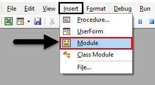
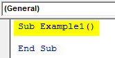
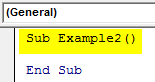
Step 2: Write the subprocedure of VBA Variable Range.
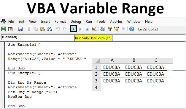
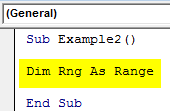
Code:
Sub Example1()

End Sub
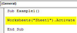
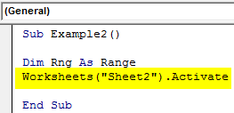
Step 3: Now here is a key part to remember that whatever procedure we write VBA executes it in the active sheet or the active worksheet, so in order to run the different procedures on the different worksheets we need to activate them first using the Activate method.
Code:
Sub Example1()

Worksheets("Sheet1").Activate

End Sub
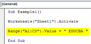
Step 4: Now let us begin the simple operation by assigning a custom value to the cell of the worksheet 1 using the range property method.
Code:
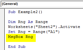
Sub Example1()

Worksheets("Sheet1").Activate
Range("A1:C3").Value = " EDUCBA "

End Sub
Step 5: Run the code by pressing the F5 key or by clicking on the Play Button. Once we execute the code we can see the value in Sheet 1 as follows.
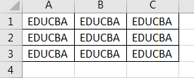
We can see that in our code we chose the cells from A1:C3 to have these custom values, this example was the basic representation of what we can do with the range property method.
VBA Variable Range – Example #2
Now let us use Range as a variable in VBA, we can use range as variable and set the variable with the values using the range property method. In this example, we will discuss how to use the range variable to fetch data from a cell and display it on the screen.
Step 1: We will begin our next example in the same module we have inserted so we do not need to insert a new module for every procedure. Below the first code initiate another subprocedure.
Code:
Sub Example2()

End Sub
Step 2: Let us set a variable as a Range data type so that it can hold or store a range of values.
Code:
Sub Example2()

Dim Rng As Range

End Sub
Step 3: Now we have discussed earlier the importance of activating a worksheet before using it for our example so we need to activate the Sheet 2.
Code:
Sub Example2()

Dim Rng As Range
Worksheets("Sheet2").Activate

End Sub
Step 4: Before we begin to our next code let us first see what is in the value of cell A1 in sheet 2.
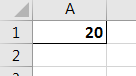
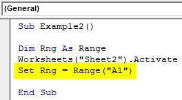
Step 5: We can see that there is data in cell A1 so we will use the Set statement to assign the value of cell A1 to our variable using the range property method.
Code:
Sub Example2()

Dim Rng As Range
Worksheets("Sheet2").Activate
Set Rng = Range("A1")

End Sub
Step 6: Now in order to display the value which has been stored in our variable let us use the msgbox function as follows in the image below.
Code:
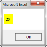
Sub Example2()

Dim Rng As Range
Worksheets("Sheet2").Activate
Set Rng = Range("A1")
MsgBox Rng

End Sub
Step 7: Now once we execute the above code we get the following result.
VBA Variable Range – Example #3
In this example, we will use a variable as a range to select a few cells from a sheet 3.
Step 1: The defining of the subprocedure will be same as for all the codes above, let us begin right below the example 3 in the same module as shown below.
Code:
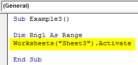
Sub Example3()

End Sub
Step 2: Now declare a variable as Range data type to store the values of a range.
Code:
Sub Example3()

Dim Rng1 As Range

End Sub
Step 3: Since we are going to execute the procedure in sheet 3 let us activate Sheet 3 first.
Code:
Sub Example3()

Dim Rng1 As Range
Worksheets("Sheet3").Activate

End Sub
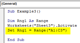
Step 4: Now use the set statement to assign a range value to our variable with the help of the range property method.
Code:
Sub Example3()

Dim Rng1 As Range
Worksheets("Sheet3").Activate
Set Rng1 = Range("A1:C3")
Rng1.Select

End Sub
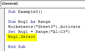
Step 5: Now let us use the select statement to select the range in the variable.
Code:
Sub Example3()

Dim Rng1 As Range
Worksheets("Sheet3").Activate
Set Rng1 = Range("A1:C3")
Rng1.Select

End Sub
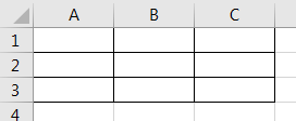
Step 6: When we execute the code and go to sheet 3 we can see the following result.
VBA Variable Range – Example #4
Now let us use a variable range to assign some values to a specific range and change their font in the meanwhile.
Step 1: In the same module below example 3 we will set another procedure named Example4.
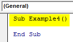
Code:
Sub Example4()

End Sub
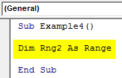
Step 2: Now set a variable as Range data type to store the values of a range.
Code:
Sub Example4()

Dim Rng2 As Range

End Sub
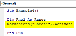
Step 3: Since we are going to execute the procedure in Sheet4 first let us activate Sheet4.
Code:
Sub Example4()

Dim Rng2 As Range
Worksheets("Sheet4").Activate

End Sub
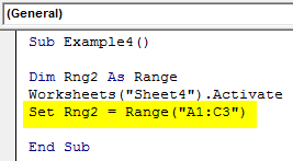
Step 4: Now use the set statement to assign a range value to our variable with the help of the range property method as shown below.
Code:
Sub Example4()

Dim Rng2 As Range
Worksheets("Sheet4").Activate
Set Rng2 = Range("A1:C3")

End Sub
Step 5: Now we will use the Value property of a range method to assign a value to that range.
Code:
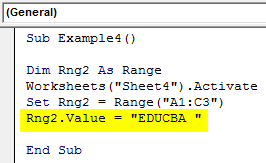
Sub Example4()

Dim Rng2 As Range
Worksheets("Sheet4").Activate
Set Rng2 = Range("A1:C3")
Rng2.Value = "EDUCBA "

End Sub
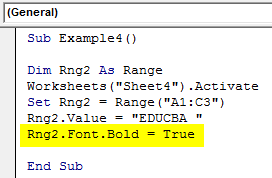
Step 6: Now let us change the font for the range to make it bold with the following code.
Code:
Sub Example4()

Dim Rng2 As Range
Worksheets("Sheet4").Activate
Set Rng2 = Range("A1:C3")
Rng2.Value = "EDUCBA "
Rng2.Font.Bold = True

End Sub
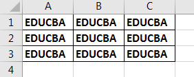
Step 7: When we execute this code we can see the following result in sheet 4 as shown below.
Explanation of VBA Variable Range:
Now with the above examples, we can see how useful is the variable range in our coding. Let me give an example of finding the last row in any sheet. We cannot do that with a normal range property method for that we need a variable as a range because the range property method will be static and the last row will not be identified once the data changes but using variable range we make it dynamic so that the values can also change.
How to Use the VBA Variable Range?
Let me explain another example on how to use variable range in real time code. Let us say we have different values in Sheet5 as shown below.
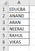
And I want to find which row has value “EDUCBA”, we want the row number to be displayed.
Code:
Sub Example5()

Dim ws As Worksheet
Dim FoundCell As Range
Dim WTF As String
Dim k As Integer
Set ws = Worksheets("Sheet5")
WTF = Range("A1").Value
Set FoundCell = ws.Range("A:A").Find(What:=WTF)
k = FoundCell.Row
MsgBox "Found the Value At Row " & k

End Sub
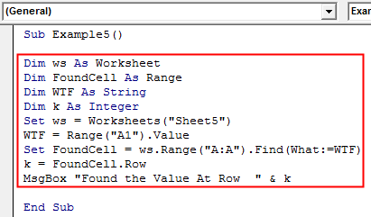
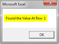
When we execute the code the following result is displayed.
Let me explain the code, the variable Foundcell is a variable range that searches for the value of A1 in a whole range A:A and when the value is found it displays the row number with the Row method.
Things to Remember
- Variable range is a variable with range data type.
- It is defined as the same as the Dim Statement.
- We use the Set statement to assign a range to the variable.
- Range Property method is used to access the values for the range variable.
Recommended Articles
This is a guide to VBA Variable Range. Here we discuss how to set variable range in Excel using VBA code along with practical examples and downloadable excel template. You can also go through our other suggested articles –
- VBA Selection Range
- VBA IF Statements
- VBA Variable Declaration
- VBA Format Number