
| title | keywords | f1_keywords | ms.prod | api_name | ms.assetid | ms.date | ms.localizationpriority |
|---|---|---|---|---|---|---|---|
|
WorksheetFunction.Index method (Excel) |
vbaxl10.chm137090 |
vbaxl10.chm137090 |
excel |
Excel.WorksheetFunction.Index |
4656985a-2864-93ed-31c7-e7a551d68e96 |
05/23/2019 |
medium |
WorksheetFunction.Index method (Excel)
Returns a value or the reference to a value from within a table or range. There are two forms of the Index function: the array form and the reference form.
Syntax
expression.Index (Arg1, Arg2, Arg3, Arg4)
expression A variable that represents a WorksheetFunction object.
Parameters
| Name | Required/Optional | Data type | Description |
|---|---|---|---|
| Arg1 | Required | Variant | Array or Reference — a range of cells or an array constant. For references, it is the reference to one or more cell ranges. |
| Arg2 | Required | Double | Row_num — selects the row in array from which to return a value. If row_num is omitted, column_num is required. For references, the number of the row in reference from which to return a reference. |
| Arg3 | Optional | Variant | Column_num — selects the column in array from which to return a value. If column_num is omitted, row_num is required. For reference, the number of the column in reference from which to return a reference. |
| Arg4 | Optional | Variant | Area_num — only used when returning references. Selects a range in reference from which to return the intersection of row_num and column_num. The first area selected or entered is numbered 1, the second is 2, and so on. If area_num is omitted, Index uses area 1. |
Return value
Variant
Remarks
Array form
Returns the value of an element in a table or an array, selected by the row and column number indexes.
Use the array form if the first argument to Index is an array constant.
If both the row_num and column_num arguments are used, Index returns the value in the cell at the intersection of row_num and column_num.
If you set row_num or column_num to 0 (zero), Index returns the array of values for the entire column or row, respectively. To use values returned as an array, enter the Index function as an array formula in a horizontal range of cells for a row, and in a vertical range of cells for a column. To enter an array formula, press Ctrl+Shift+Enter.
Row_num and column_num must point to a cell within array; otherwise, Index returns the #REF! error value.
Reference form
Returns the reference of the cell at the intersection of a particular row and column. If the reference is made up of nonadjacent selections, you can pick the selection to look in. If each area in reference contains only one row or column, the row_num or column_num argument, respectively, is optional. For example, for a single row reference, use INDEX(reference,column_num).
After reference and area_num have selected a particular range, row_num and column_num select a particular cell: row_num 1 is the first row in the range, column_num 1 is the first column, and so on. The reference returned by Index is the intersection of row_num and column_num.
If you set row_num or column_num to 0 (zero), Index returns the reference for the entire column or row, respectively.
Row_num, column_num, and area_num must point to a cell within reference; otherwise, Index returns the #REF! error value. If row_num and column_num are omitted, Index returns the area in reference specified by area_num.
The result of the Index function is a reference and is interpreted as such by other formulas. Depending on the formula, the return value of Index may be used as a reference or as a value. For example, the formula CELL("width",INDEX(A1:B2,1,2)) is equivalent to CELL("width",B1). The CELL function uses the return value of Index as a cell reference. On the other hand, a formula such as 2*INDEX(A1:B2,1,2) translates the return value of Index into the number in cell B1.
[!includeSupport and feedback]
Indexes in Programming
“Index” is a common term used in all programming languages. It basically acts like a serial number of which an item or value can be referenced. For example, in the picture below, “Great Wall of China” is the 5th item in the series. In programming we say that its index is “5.” In some programming languages the index numbering starts with “0.” If such is the case, the index of the same “Great Wall of China” would be “4” (0, 1 , 2, 3, 4).
In general, “index” can be used to reference the values of an array or a range (in Excel).

The Index Formula in Excel
In MS Excel, index is a formula that helps us find the value in a specified array.
Syntax of the formula:
Index(< array name >, < row number >, [< col number>])
Where
- Array is an array of values (a list of one or more dimensions)/ a reference to an array.
- Row number is the row index being referred to
- Col number is the column index being referred to
Example 1
In this example we are trying to find the value in the 7th position of the lookup range (the parameter used in the formula).
Here the range is B2 to B9 i.e. Starting from the value “Taj Mahal” (position 1) in B2 until “Great Pyramid of Giza” (position  in B9. Visually we can see that Petra is the 7th value in the selected range. Hence, it is the value returned by the formula.
Note: S.no is given in the example for easy understanding and it has nothing to do with the Index formula.

Example 2
Let us try to find the price of the 7th item (“Sambar Idly”) sold at a snack bar. There are two columns here, one with the list of items and the other with the respective price.
Note: Paste this table starting with cell A1 on the Excel sheet for the formula’s range to work.
| Item | Price |
| Ice cream | 5 |
| Sweet corn | 6 |
| Spinach Candy | 8 |
| Banana Cake | 3 |
| Peas Pulao | 40 |
| Methi Roti | 30 |
| Sambar Idly with ghee | 20 |
| Veg clear Soup | 40 |
| Masala Papad | 10 |
The formula would be =INDEX(A2:B10,7,2)
Where
A2:B10 is the range of data in the table
7 because we are looking for the 7th item (row-wise)
2 because we want the price of the item. The price is in the 2nd col. And the answer would be 20.
The Index Function in VBA
The Index function in VBA is very simple. Just as in the formula, here we also have to pass the array and the position as parameters. The function then returns the value in that position.
Example 1
In the example below, there is an array of students in a class. Let us assume that we know the roll number of the student who has obtained Rank 1. We are asked to find his/her name.
Sub index_demo()

' declare variables
Dim arr_students()
Dim first_rank

' initialize the arrayarr_students = Array("John Capps", "Michel Pinny", "Kanya Dhan", "Ron Dincy", "Bella", "Mayur", "Jack finner", "Emi Thinner")

' We know that the fourth student in the array has got the first rank. We need to find his name
first_rank = Application.WorksheetFunction.Index(arr_students, 4)

'Display the name of the first rank holder in a messagebox
MsgBox first_rank & " is the student who got the first rank."

End Sub
Example explained:
To start with, we have declared the required variables. Then we have initiated an array (arr_students) with the list of student names as values.
In order to use the Index function, we should have the array and required position number as parameters. As we have created the array already (arr_students) and we know that the name of the student with the roll number “4” is to be fetched, we proceed to use the function.
Application.WorksheetFunction.Index (arr_students, 4)
Application refers to the Excel application being used currently.
Worksheetfunction refers to the bunch of functions offered by Excel for any worksheet.
Index is also a worksheetfunction which we are learning to use here.
The output/return value of this function is passed/caught in the variable declared earlier — first_rank.
Finally, the value of the variable is displayed with a description in a message box.

Example 2
In this example, we will use the worksheetfunction index in VBA but the array that we refer to will be a Range of Excel cells.
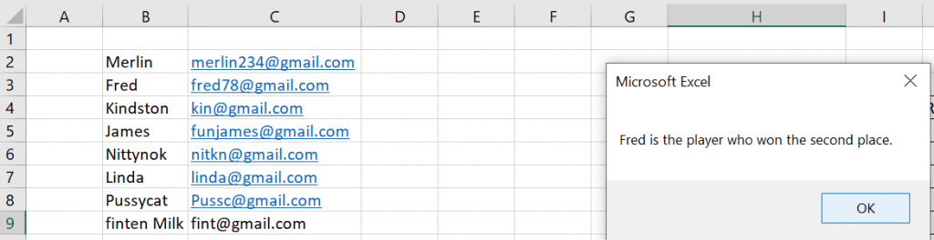
Scenario: Some sports personalities ran a race and reached the finish line in a particular order. The array of players is in the finishing order. We are asked to find the runner of the race.
Let’s try to find the person who wins the second place in the competition. This will be our position value in the function.
The range of the array is Range(“B2:B9”).
Knowing the required values, we can proceed with writing the code.
Sub index_demo2()

' declare variables
Dim arr_players()
Dim runner
' initialize the array
arr_players = Range("B2:C9")

' We know that the second player in the array is the runner. We need to find his name
runner = Application.WorksheetFunction.Index(arr_players, 2)

'Display the name of the runner in a messagebox
MsgBox runner(1) & " is the player who won the second place. His email id is " & runner(2)

End Sub
Code explained:
As mentioned in Example 1, we have declared and initialized the variables. Then we use the Index function to find runner (2nd place) of the match.
The flow of the program is the same with the difference that here we have been forced to use runner(1) to display value.
Reason: An Excel range is considered a multidimensional array. Because of this, the return value is not just a string. Instead, it is also an array. To find a value in that array, we have to specify index.
(1) is used here since there is only one value (or we have specified only 1 column in the range).
To understand it better, if we had used the range Range (“B2:C9” ) in our code, then the return value of the index would have both values in Range (“B2”) and Range(“C2”) i.e. All values of (various columns) of the second row (position parameter given in the Index function).

The image above clearly shows the value of the runner object (the returned value). It has both the name and the email address. Suppose, I want to display the email address of the runner, I will have to display runner(2) in the messagebox.
MsgBox runner(1) & " is the player who won the second place. His email id is " & runner(2)
<!-- /wp:shortcode -->
<!-- wp:image {"id":14452,"sizeSlug":"large","linkDestination":"none"} -->
<figure class="wp-block-image size-large"><img src="https://software-solutions-online.com/wp-content/uploads/2021/06/unnamed-11.png" alt="Excel message box that reads &quot;Fred is the player who won the second place. His email id is [email protected]&quot;" class="wp-image-14452"/></figure>
<!-- /wp:image -->
<!-- wp:heading {"level":3} -->
<h3>Example 3</h3>
<!-- /wp:heading -->
<!-- wp:paragraph -->
<p>In the example below, we get the capital of a state whose index is known. So, we are using an array of two dimensions. If we use formula, we refer to the 4<sup>th</sup> row and 2<sup>nd</sup> column of the selected range. So the value of the cell turns out to be “Patna”.</p>
<!-- /wp:paragraph -->
<!-- wp:image {"id":14457,"sizeSlug":"large","linkDestination":"none"} -->
<figure class="wp-block-image size-large"><img src="https://software-solutions-online.com/wp-content/uploads/2021/06/unnamed-12-1024x266.png" alt="Example of using array to find capital states." class="wp-image-14457"/></figure>
<!-- /wp:image -->
<!-- wp:paragraph -->
<p>Let us do the same using VBA.</p>
<!-- /wp:paragraph -->
<!-- wp:shortcode -->
Sub IndexMatch_demo1()
' declare variables
Dim required_pos, str_capital, arr_states_cap, capital_col
' initialize variables
required_pos = 4
capital_col = 2
arr_states_cap = Range("B2:C16")
'use the function to get the capital
str_capital = Application.WorksheetFunction.Index([arr_states_cap], required_pos, 2)
' display the result
MsgBox str_capital
End Sub
Code explained:
Post declaration and initialization of variables, the Index function is used to get the value in the 4th row, 2nd column of the selected state, capital range of cells on the Excel sheet.
Finally, the output that we see in the message box would be “Patna” which is the capital of Bihar.
The Match Formula and Function
Here is my article about the Match formula in Excel and Match function in VBA:
Using the Match Function in VBA and Excel – VBA and VB.Net Tutorials, Education and Programming Services (software-solutions-online.com)
Using the Index Function with the Match Function
As we have already understood, the Index function gives the value in the known index of an array. The Match function does the opposite. It provides the index value of an item in an array or range of values.
It is possible to use one of these functions within the other. i.e. Match within Index (or) Index within Match.
Example 1
Here is a table that has details of States, Capitals and another column to describe when it was formed (“Founded on”). We are asked to find the “Founded on” value of the state “Maharashtra”.
Let us assume that we do not know its index. So, initially we will use the Match function to find its index.
Once we get that index, using Index we can get the respective values of that index (rows) against all columns.

Sub IndexMatch_demo()

'declare variables
Dim strstate, arr_states, arr_capitals, arr_founded, rowposition_state, str_capital, str_founded

' initialize variables ( set values for them )
strstate = "Maharashtra"
arr_states = Range("B2:B30")
arr_capitals = Range("C2:C30")
arr_founded = Range("D2:D30")

' find the position of the state in the first array ( 0 here states an exact match)
rowposition_state = Application.WorksheetFunction.Match(strstate, ([arr_states]), 0)

'Find the respective capital and "founded on" values of the said state.
str_capital = Application.WorksheetFunction.Index([arr_capitals], rowposition_state)
str_founded = Application.WorksheetFunction.Index([arr_founded], rowposition_state)

' display all values
Debug.Print str_capital(1)
Debug.Print str_founded(1)

End Sub
Code explained:
The required variables are first declared and then initialized. From these lines, we infer that we are supposed to find the capital and “Founded on” values of the state “Maharashtra.” So, using the Match function in VBA, we find the position of the state ”Maharashtra.” Then using the same value as the index, we find the capital and “Founded on” values from the respective arrays and display the same in the Immediate window (using the debug.print statement).
In order to explain this further, three arrays were created in the example. If the ranges quoted for each of these arrays are not within the same range ( row values), then this concept of using the same index (row num here) for finding values in other arrays will not work. So, let us redo the same with one range as a subset of another range to understand the concept better.
Sub IndexMatch_demo3()

'declare variables
Dim strstate, arr_states, start_pos, end_pos, rowposition_state, str_capital, arr_states_captials

' initialize variables ( set values for them )
strstate = "Maharashtra"
start_pos = 2
end_pos = 30

'dynamic defining of the arrays from the excel sheet. The rows values are not hardcoded here.
arr_states_captials = Range("B" & start_pos & ":D" & end_pos)
arr_states = Range("B" & start_pos & ":B" & end_pos)

' find the position of the state in the states array ( 0 here states an exact match)
rowposition_state = Application.WorksheetFunction.Match(strstate, [arr_states], 0)

'Find the respective capital and "founded on" values of the said state.
str_capital = Application.WorksheetFunction.Index([arr_states_captials], rowposition_state, 2)
str_founded = Application.WorksheetFunction.Index([arr_states_captials], rowposition_state, 3)

' display all values
Debug.Print str_capital
Debug.Print str_founded

End Sub
Code explained:
The difference in this modified code lies in the dynamic building of array range. A single dimensional array is defined in order to find the index using the Match function. Then we find the respective values from the other two columns. The Index function here uses both the row position and col position parameter since the array is multidimensional (a complete picture of this is available in the image above).
Conclusion
In my experience, I see that the Index function can be used with multidimensional arrays but when it comes to the Match function, multidimensional arrays have to be sliced using loops and conditions before being passed as parameters. Using a combination of both these functions (Index and Match), it is possible and easy to point to any value/index/any target in a table or an array or a range of Excel cells. Using them wisely can produce great results.
Содержание
- WorksheetFunction.Index method (Excel)
- Syntax
- Parameters
- Return value
- Remarks
- Array form
- Reference form
- Support and feedback
- Метод WorksheetFunction.Index (Excel)
- Синтаксис
- Параметры
- Возвращаемое значение
- Примечания
- Форма массива
- Форма ссылок
- Поддержка и обратная связь
- Name already in use
- VBA-Docs / api / Excel.WorksheetFunction.Index.md
- Name already in use
- VBA-content / VBA / Excel-VBA / articles / worksheetfunction-index-method-excel.md
WorksheetFunction.Index method (Excel)
Returns a value or the reference to a value from within a table or range. There are two forms of the Index function: the array form and the reference form.
Syntax
expression A variable that represents a WorksheetFunction object.
Parameters
| Name | Required/Optional | Data type | Description |
|---|---|---|---|
| Arg1 | Required | Variant | Array or Reference — a range of cells or an array constant. For references, it is the reference to one or more cell ranges. |
| Arg2 | Required | Double | Row_num — selects the row in array from which to return a value. If row_num is omitted, column_num is required. For references, the number of the row in reference from which to return a reference. |
| Arg3 | Optional | Variant | Column_num — selects the column in array from which to return a value. If column_num is omitted, row_num is required. For reference, the number of the column in reference from which to return a reference. |
| Arg4 | Optional | Variant | Area_num — only used when returning references. Selects a range in reference from which to return the intersection of row_num and column_num. The first area selected or entered is numbered 1, the second is 2, and so on. If area_num is omitted, Index uses area 1. |
Return value
Variant
Array form
Returns the value of an element in a table or an array, selected by the row and column number indexes.
Use the array form if the first argument to Index is an array constant.
If both the row_num and column_num arguments are used, Index returns the value in the cell at the intersection of row_num and column_num.
If you set row_num or column_num to 0 (zero), Index returns the array of values for the entire column or row, respectively. To use values returned as an array, enter the Index function as an array formula in a horizontal range of cells for a row, and in a vertical range of cells for a column. To enter an array formula, press Ctrl+Shift+Enter.
Row_num and column_num must point to a cell within array; otherwise, Index returns the #REF! error value.
Reference form
Returns the reference of the cell at the intersection of a particular row and column. If the reference is made up of nonadjacent selections, you can pick the selection to look in. If each area in reference contains only one row or column, the row_num or column_num argument, respectively, is optional. For example, for a single row reference, use INDEX(reference,column_num).
After reference and area_num have selected a particular range, row_num and column_num select a particular cell: row_num 1 is the first row in the range, column_num 1 is the first column, and so on. The reference returned by Index is the intersection of row_num and column_num.
If you set row_num or column_num to 0 (zero), Index returns the reference for the entire column or row, respectively.
Row_num, column_num, and area_num must point to a cell within reference; otherwise, Index returns the #REF! error value. If row_num and column_num are omitted, Index returns the area in reference specified by area_num.
The result of the Index function is a reference and is interpreted as such by other formulas. Depending on the formula, the return value of Index may be used as a reference or as a value. For example, the formula CELL(«width»,INDEX(A1:B2,1,2)) is equivalent to CELL(«width»,B1) . The CELL function uses the return value of Index as a cell reference. On the other hand, a formula such as 2*INDEX(A1:B2,1,2) translates the return value of Index into the number in cell B1.
Support and feedback
Have questions or feedback about Office VBA or this documentation? Please see Office VBA support and feedback for guidance about the ways you can receive support and provide feedback.
Источник
Метод WorksheetFunction.Index (Excel)
Возвращает значение или ссылку на значение из таблицы или диапазона. Существует две формы функции Index : форма массива и форма ссылки.
Синтаксис
Выражение Переменная, представляющая объект WorksheetFunction .
Параметры
| Имя | Обязательный или необязательный | Тип данных | Описание |
|---|---|---|---|
| Arg1 | Обязательный | Variant | Массив или ссылка — диапазон ячеек или константы массива. Для ссылок это ссылка на один или несколько диапазонов ячеек. |
| Arg2 | Обязательный | Double | Row_num — выбирает строку в массиве, из которой возвращается значение. Если row_num опущен, требуется column_num. Для ссылок — номер строки в ссылке, из которой возвращается ссылка. |
| Arg3 | Необязательный | Variant | Column_num — выбирает столбец в массиве, из которого возвращается значение. Если column_num опущен, требуется row_num. Для справки— номер столбца в ссылке, из которого возвращается ссылка. |
| Arg4 | Необязательный | Variant | Area_num — используется только при возврате ссылок. Выбирает диапазон в ссылке, из которого возвращается пересечение row_num и column_num. Первая выбранная или введенная область нумеруется 1, вторая — 2 и т. д. Если area_num опущен, индекс использует область 1. |
Возвращаемое значение
Variant
Примечания
Форма массива
Возвращает значение элемента в таблице или массиве, выбранное индексами номеров строк и столбцов.
Используйте форму массива, если первый аргумент index является константой массива.
Если используются аргументы row_num и column_num, индекс возвращает значение в ячейке на пересечении row_num и column_num.
Если для row_num или column_num задано значение 0 (ноль), индекс возвращает массив значений для всего столбца или строки соответственно. Чтобы использовать значения, возвращаемые в качестве массива, введите функцию Index в качестве формулы массива в горизонтальном диапазоне ячеек для строки и в вертикальном диапазоне ячеек для столбца. Чтобы ввести формулу массива, нажмите клавиши CTRL+SHIFT+ВВОД.
Row_num и column_num должны указывать на ячейку в массиве; В противном случае индекс возвращает #REF! значение ошибки.
Форма ссылок
Возвращает ссылку на ячейку на пересечении определенной строки и столбца. Если ссылка состоит из несмежных выделений, можно выбрать выделение для поиска. Если каждая область ссылки содержит только одну строку или столбец, аргумент row_num или column_num соответственно является необязательным. Например, для ссылки на одну строку используйте index(reference,column_num).
После того как ссылка и area_num выбрали определенный диапазон, row_num и column_num выбрать определенную ячейку: row_num 1 — первая строка диапазона, column_num 1 — первый столбец и т. д. Ссылка, возвращаемая индексом , является пересечением row_num и column_num.
Если row_num или column_num задано значение 0 (ноль), индекс возвращает ссылку на весь столбец или строку соответственно.
Row_num, column_num и area_num должны указывать на ячейку в ссылке; В противном случае индекс возвращает #REF! значение ошибки. Если row_num и column_num опущены, индекс возвращает область в ссылке, указанную area_num.
Результат функции Index является ссылкой и интерпретируется как таковой другими формулами. В зависимости от формулы возвращаемое значение Index может использоваться в качестве ссылки или в качестве значения. Например, формула CELL(«width»,INDEX(A1:B2,1,2)) эквивалентна CELL(«width»,B1) . Функция CELL использует возвращаемое значение Index в качестве ссылки на ячейку. С другой стороны, формула, например 2*INDEX(A1:B2,1,2) , преобразует возвращаемое значение Index в число в ячейке B1.
Поддержка и обратная связь
Есть вопросы или отзывы, касающиеся Office VBA или этой статьи? Руководство по другим способам получения поддержки и отправки отзывов см. в статье Поддержка Office VBA и обратная связь.
Источник
Name already in use
VBA-Docs / api / Excel.WorksheetFunction.Index.md
- Go to file T
- Go to line L
- Copy path
- Copy permalink
Copy raw contents
Copy raw contents
WorksheetFunction.Index method (Excel)
Returns a value or the reference to a value from within a table or range. There are two forms of the Index function: the array form and the reference form.
expression A variable that represents a WorksheetFunction object.
| Name | Required/Optional | Data type | Description |
|---|---|---|---|
| Arg1 | Required | Variant | Array or Reference — a range of cells or an array constant. For references, it is the reference to one or more cell ranges. |
| Arg2 | Required | Double | Row_num — selects the row in array from which to return a value. If row_num is omitted, column_num is required. For references, the number of the row in reference from which to return a reference. |
| Arg3 | Optional | Variant | Column_num — selects the column in array from which to return a value. If column_num is omitted, row_num is required. For reference, the number of the column in reference from which to return a reference. |
| Arg4 | Optional | Variant | Area_num — only used when returning references. Selects a range in reference from which to return the intersection of row_num and column_num. The first area selected or entered is numbered 1, the second is 2, and so on. If area_num is omitted, Index uses area 1. |
Variant
Returns the value of an element in a table or an array, selected by the row and column number indexes.
Use the array form if the first argument to Index is an array constant.
If both the row_num and column_num arguments are used, Index returns the value in the cell at the intersection of row_num and column_num.
If you set row_num or column_num to 0 (zero), Index returns the array of values for the entire column or row, respectively. To use values returned as an array, enter the Index function as an array formula in a horizontal range of cells for a row, and in a vertical range of cells for a column. To enter an array formula, press Ctrl+Shift+Enter.
Row_num and column_num must point to a cell within array; otherwise, Index returns the #REF! error value.
Returns the reference of the cell at the intersection of a particular row and column. If the reference is made up of nonadjacent selections, you can pick the selection to look in. If each area in reference contains only one row or column, the row_num or column_num argument, respectively, is optional. For example, for a single row reference, use INDEX(reference,column_num).
After reference and area_num have selected a particular range, row_num and column_num select a particular cell: row_num 1 is the first row in the range, column_num 1 is the first column, and so on. The reference returned by Index is the intersection of row_num and column_num.
If you set row_num or column_num to 0 (zero), Index returns the reference for the entire column or row, respectively.
Row_num, column_num, and area_num must point to a cell within reference; otherwise, Index returns the #REF! error value. If row_num and column_num are omitted, Index returns the area in reference specified by area_num.
The result of the Index function is a reference and is interpreted as such by other formulas. Depending on the formula, the return value of Index may be used as a reference or as a value. For example, the formula CELL(«width»,INDEX(A1:B2,1,2)) is equivalent to CELL(«width»,B1) . The CELL function uses the return value of Index as a cell reference. On the other hand, a formula such as 2*INDEX(A1:B2,1,2) translates the return value of Index into the number in cell B1.
Источник
Name already in use
VBA-content / VBA / Excel-VBA / articles / worksheetfunction-index-method-excel.md
- Go to file T
- Go to line L
- Copy path
- Copy permalink
Copy raw contents
Copy raw contents
WorksheetFunction.Index Method (Excel)
Returns a value or the reference to a value from within a table or range. There are two forms of the INDEX function: the array form and the reference form.
expression . Index( Arg1 , Arg2 , Arg3 , Arg4 )
expression A variable that represents a WorksheetFunction object.
| Name | Required/Optional | Data Type | Description |
|---|---|---|---|
| Arg1 | Required | Variant | Array or Reference — a range of cells or an array constant. For references, it is the reference to one or more cell ranges. |
| Arg2 | Required | Double | Row_num — selects the row in array from which to return a value. If row_num is omitted, column_num is required. For references, the number of the row in reference from which to return a reference |
| Arg3 | Optional | Variant | Column_num — selects the column in array from which to return a value. If column_num is omitted, row_num is required. For reference, the number of the column in reference from which to return a reference. |
| Arg4 | Optional | Variant | Area_num — only used when returning references. Selects a range in reference from which to return the intersection of row_num and column_num. The first area selected or entered is numbered 1, the second is 2, and so on. If area_num is omitted, INDEX uses area 1. |
Returns the value of an element in a table or an array, selected by the row and column number indexes.
Use the array form if the first argument to INDEX is an array constant.
If both the row_num and column_num arguments are used, INDEX returns the value in the cell at the intersection of row_num and column_num.
If you set row_num or column_num to 0 (zero), INDEX returns the array of values for the entire column or row, respectively. To use values returned as an array, enter the INDEX function as an array formula in a horizontal range of cells for a row, and in a vertical range of cells for a column. To enter an array formula, press CTRL+SHIFT+ENTER.
Row_num and column_num must point to a cell within array; otherwise, INDEX returns the #REF! error value.
Returns the reference of the cell at the intersection of a particular row and column. If the reference is made up of nonadjacent selections, you can pick the selection to look in. If each area in reference contains only one row or column, the row_num or column_num argument, respectively, is optional. For example, for a single row reference, use INDEX(reference,,column_num).
After reference and area_num have selected a particular range, row_num and column_num select a particular cell: row_num 1 is the first row in the range, column_num 1 is the first column, and so on. The reference returned by INDEX is the intersection of row_num and column_num.
If you set row_num or column_num to 0 (zero), INDEX returns the reference for the entire column or row, respectively.
Row_num, column_num, and area_num must point to a cell within reference; otherwise, INDEX returns the #REF! error value. If row_num and column_num are omitted, INDEX returns the area in reference specified by area_num.
The result of the INDEX function is a reference and is interpreted as such by other formulas. Depending on the formula, the return value of INDEX may be used as a reference or as a value. For example, the formula CELL(«width»,INDEX(A1:B2,1,2)) is equivalent to CELL(«width»,B1). The CELL function uses the return value of INDEX as a cell reference. On the other hand, a formula such as 2*INDEX(A1:B2,1,2) translates the return value of INDEX into the number in cell B1.
Источник
The INDEX and MATCH function in VBA combination is the alternative to the VLOOKUP function in excel. In VBA, we do not have the luxury of using the INDEX and MATCH functionThe MATCH function looks for a specific value and returns its relative position in a given range of cells. The output is the first position found for the given value. Being a lookup and reference function, it works for both an exact and approximate match. For example, if the range A11:A15 consists of the numbers 2, 9, 8, 14, 32, the formula “MATCH(8,A11:A15,0)” returns 3. This is because the number 8 is at the third position.
read more directly because these two functions are not part of the VBA built-in functionsVBA functions serve the primary purpose to carry out specific calculations and to return a value. Therefore, in VBA, we use syntax to specify the parameters and data type while defining the function. Such functions are called user-defined functions.read more. However, we can still use them as part of the worksheet function class.
Table of contents
- Index Match in VBA
- How to Use Index Match in VBA? (Step by Step)
- Recommended Articles

You are free to use this image on your website, templates, etc, Please provide us with an attribution linkArticle Link to be Hyperlinked
For eg:
Source: VBA Index Match (wallstreetmojo.com)
How to Use Index Match in VBA? (Step by Step)
You can download this VBA Index Match Excel Template here – VBA Index Match Excel Template
For example, look at the below data.

In the above data, the lookup value is the “Department” name. Based on this department name, we need to extract the salary amount.
But the problem here is that the result column is there in the first, and the lookup value column is the result column. So, in this case, VLOOKUP cannot fetch the salary amount because VLOOKUP worksThe VLOOKUP excel function searches for a particular value and returns a corresponding match based on a unique identifier. A unique identifier is uniquely associated with all the records of the database. For instance, employee ID, student roll number, customer contact number, seller email address, etc., are unique identifiers.
read more only from right to left, not from left to right.
In these cases, we need to use the combination formula of the VBA INDEX and MATCH function. But, first, let us perform the task of finding the salary amount of each department in the VBA codeVBA code refers to a set of instructions written by the user in the Visual Basic Applications programming language on a Visual Basic Editor (VBE) to perform a specific task.read more.
Step 1: Start the sun routine.
Step 2: Declare the VBA IntegerIn VBA, an integer is a data type that may be assigned to any variable and used to hold integer values. In VBA, the bracket for the maximum number of integer variables that can be kept is similar to that in other languages. Using the DIM statement, any variable can be defined as an integer variable.read more variable.
Code:
Sub INDEX_MATCH_Example1()

Dim k As Integer

End Sub

Step 3: Now, open For Next Loop in VBAAll programming languages make use of the VBA For Next loop. After the FOR statement, there is a criterion in this loop, and the code loops until the criteria are reached. read more.
Code:
Sub INDEX_MATCH_Example1()

Dim k As Integer

For k = 2 To 5


Next k

End Sub

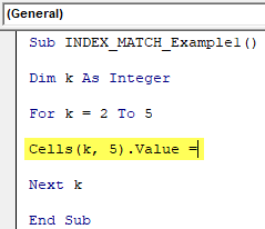
Step 4: Inside the VBA loopA VBA loop in excel is an instruction to run a code or repeat an action multiple times.read more, execute the formula. In the 5th column, we need to apply the formula, so the code is CELLS (k,5).Value =
Code:
Sub INDEX_MATCH_Example1()

Dim k As Integer

For k = 2 To 5

Cells(k, 5).Value =

Next k

End Sub
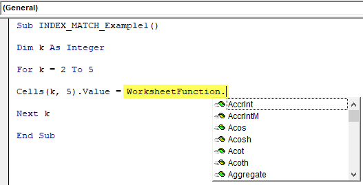
Step 5: We must apply that cell’s VBA INDEX and MATCH formula. As we said, we need to use these functions as a Worksheet Function in VBAThe worksheet function in VBA is used when we need to refer to a specific worksheet. When we create a module, the code runs in the currently active sheet of the workbook, but we can use the worksheet function to run the code in a particular worksheet.read more class, so open the worksheet function class.
Code:
Sub INDEX_MATCH_Example1()

Dim k As Integer

For k = 2 To 5

Cells(k, 5).Value = WorksheetFunction.

Next k

End Sub
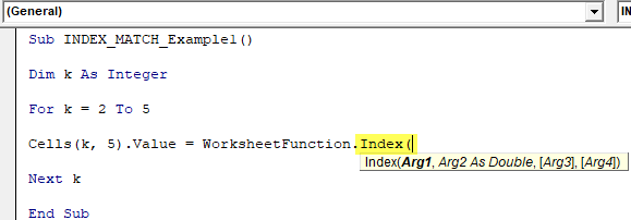
Step 6: After entering the worksheet function class, we can see all the available worksheet functions, so select the INDEX function.
Code:
Sub INDEX_MATCH_Example1()

Dim k As Integer

For k = 2 To 5

Cells(k, 5).Value = WorksheetFunction.Index(

Next k

End Sub
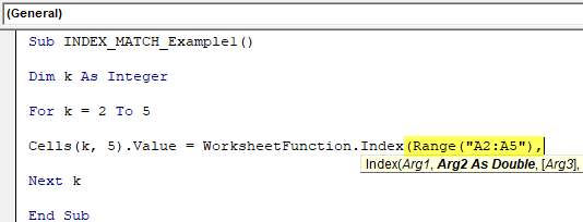
Step 7: While using the worksheet function in VBA, you must be sure of the arguments of the formula. The first argument is an array, i.e., from which column we need the result. In this case, we need the result from A2 to A5.
Code:
Sub INDEX_MATCH_Example1()

Dim k As Integer

For k = 2 To 5

Cells(k, 5).Value = WorksheetFunction.Index(Range("A2:A5"),

Next k

End Sub
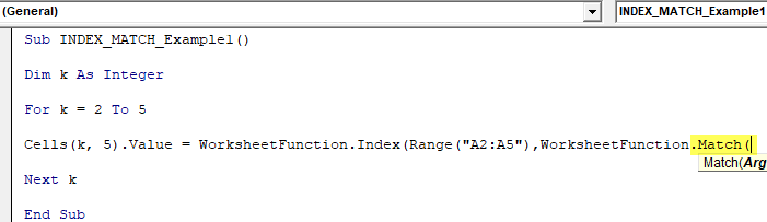
Step 8: Next up is from which row number we need the result. As we have seen in the earlier example, we cannot manually supply the row number every time. So, use the MATCH function.
To use the MATCH function again, we need to open the Worksheet function class.
Code:
Sub INDEX_MATCH_Example1()

Dim k As Integer

For k = 2 To 5

Cells(k, 5).Value = WorksheetFunction.Index(Range("A2:A5"),
WorksheetFunction.Match(

Next k

End Sub
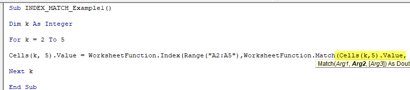
Step 9: The MATCH function’s first argument is the LOOKUP value; here, our lookup value is department names; it is there in the cells (2, 4).
Since every time the row number changes, we can supply the variable “k” in place of manual row number 2. Cells (k, 4).Value
Code:
Sub INDEX_MATCH_Example1()

Dim k As Integer

For k = 2 To 5

Cells(k, 5).Value = WorksheetFunction.Index(Range("A2:A5"),
WorksheetFunction.Match(Cells(k,5).Value,

Next k

End Sub
Step 10: Next, we need to mention the department value range, i.e., Range (“B2:B5”).
Code:
Sub INDEX_MATCH_Example1()

Dim k As Integer

For k = 2 To 5

Cells(k, 5).Value = WorksheetFunction.Index(Range("A2:A5"),
WorksheetFunction.Match(Cells(k,5).Value,Range("B2:B5"),
Next k
End Sub
Step 11: Next, put the argument as 0 because we need an exact match and close the brackets.
Code:
Sub INDEX_MATCH_Example1()

Dim k As Integer

For k = 2 To 5

Cells(k, 5).Value = WorksheetFunction.Index(Range("A2:A5"),
WorksheetFunction.Match(Cells(k, 4).Value, Range("B2:B5"), 0))
Next k
End Sub
We have now completed the coding part. Let us run the code to have the result in column 5.

So, we got the result.
We can use this formula as an alternative to the VLOOKUP functionTo reference data in columns from right to left, we can combine the index and match functions, which is one of the best Excel alternatives to Vlookup.read more.
Recommended Articles
This article is a guide to VBA Index Match. Here, we learn how to use the Index Match function in VBA as an alternative to VLOOKUP, examples, and download templates. Below are some useful Excel articles related to VBA: –
- VBA Value
- String Array in VBA
- VBA Match Function
- Arrays Function in VBA