
На чтение 11 мин. Просмотров 34.3k.
Итог: научиться создавать макросы, использовать фильтры на диапазоны и таблицы с помощью метода AutoFilter VBA. Статья содержит ссылки на примеры для фильтрации различных типов данных, включая текст, цифры, даты, цвета и значки.
Уровень мастерства: средний

Содержание
- Скачать файл
- Написание макросов для фильтров
- Макро-рекордер — твой друг (или враг)
- Метод автофильтрации
- Написание кода автофильтра
- Автофильтр не является дополнением
- Как установить номер поля динамически
- Используйте таблицы Excel с фильтрами
- Фильтры и типы данных
- Почему метод автофильтрации такой сложный?
Скачать файл
Файл Excel, содержащий код, можно скачать ниже. Этот файл содержит код для фильтрации различных типов данных и типов фильтров.
![]() VBA AutoFilters Guide.xlsm (100.5 KB)
VBA AutoFilters Guide.xlsm (100.5 KB)
Написание макросов для фильтров
Фильтры являются отличным инструментом для анализа данных в
Excel. Для большинства аналитиков и частых пользователей Excel фильтры являются
частью нашей повседневной жизни. Мы используем раскрывающиеся меню фильтров для
применения фильтров к отдельным столбцам в наборе данных. Это помогает нам
связывать цифры с отчетами и проводить исследование наших данных.

Фильтрация также может быть трудоемким процессом. Особенно,
когда мы применяем фильтры к нескольким столбцам на больших листах или фильтруем
данные, чтобы затем копировать / вставлять их в другие листы или книги.
В этой статье объясняется, как создавать макросы для
автоматизации процесса фильтрации. Это обширное руководство по методу
автофильтра в VBA.
У меня также есть статьи с примерами для различных фильтров и типов данных, в том числе: пробелы, текст, числа, даты, цвета и значки, и очищающие фильтры.
Макро-рекордер — твой друг (или враг)
Мы можем легко получить код VBA для фильтров, включив
макро-рекордер, а затем применив один или несколько фильтров к диапазону /
таблице.
Вот шаги для создания макроса фильтра с помощью устройства
записи макросов:
- Включите рекордер макросов:
- Вкладка «Разработчик»> «Запись макроса».
- Дайте макросу имя, выберите, где вы хотите сохранить код, и нажмите ОК.
- Примените один или несколько фильтров, используя раскрывающиеся меню фильтров.
- Остановите рекордер.
- Откройте редактор VB (вкладка «Разработчик»> Visual Basic) для просмотра кода.
Если вы уже использовали макрос-рекордер для этого процесса,
то вы знаете, насколько он может быть полезен. Тем более, что наши критерии
фильтрации становятся более сложными.
Код будет выглядеть примерно так:
Sub Filters_Macro_Recorder()
'
' Filters_Macro_Recorder Macro
'

'
    ActiveSheet.ListObjects("tblData").Range.AutoFilter Field:=4, Criteria1:= _
        "Product 2"
    ActiveSheet.ListObjects("tblData").Range.AutoFilter Field:=4
    ActiveSheet.ListObjects("tblData").Range.AutoFilter Field:=5, Criteria1:= _
        ">=500", Operator:=xlAnd, Criteria2:="<=1000"
End Sub
Мы видим, что каждая строка использует метод AutoFilter для
применения фильтра к столбцу. Он также содержит информацию о критериях фильтра.
Мы видим, что каждая строка использует метод AutoFilter для
применения фильтра к столбцу. Он также содержит информацию о критериях фильтра.
Метод автофильтрации
Метод AutoFilter используется для очистки и применения
фильтров к одному столбцу в диапазоне или таблице в VBA. Он автоматизирует
процесс применения фильтров через выпадающие меню фильтров и делает, чтобы все работало.

Его можно использовать для применения фильтров к нескольким
столбцам путем написания нескольких строк кода, по одной для каждого столбца.
Мы также можем использовать Автофильтр, чтобы применить несколько критериев
фильтрации к одному столбцу, так же, как в выпадающем меню фильтра, установив
несколько флажков или указав диапазон дат.
Написание кода автофильтра
Вот пошаговые инструкции по написанию строки кода для автофильтра.
Шаг 1: Ссылка на диапазон или таблицу
Метод AutoFilter является частью объекта Range. Поэтому мы
должны ссылаться на диапазон или таблицу, к которым применяются фильтры на
листе. Это будет весь диапазон, к которому применяются фильтры.

Следующие примеры включают / отключают фильтры в диапазоне B3: G1000 на листе автофильтра.
Sub AutoFilter_Range()
'Автофильтр является членом объекта Range

  'Ссылка на весь диапазон, к которому применяются фильтры
  'Автофильтр включает / выключает фильтры, когда параметры не указаны.
  Sheet1.Range("B3:G1000").AutoFilter

  'Полностью квалифицированный справочник, начиная с уровня Workbook
  ThisWorkbook.Worksheets("AutoFilter Guide").Range("B3:G1000").AutoFilter

End Sub
Вот пример использования таблиц Excel.
Sub AutoFilter_Table()
'Автофильтры на таблицах работают одинаково.

Dim lo As ListObject 'Excel Table

  'Установить переменную ListObject (Table)
  Set lo = Sheet1.ListObjects(1)

  'Автофильтр является членом объекта Range
  'Родителем объекта Range является объект List
  lo.Range.AutoFilter

End Sub
Метод AutoFilter имеет 5 необязательных параметров, которые
мы рассмотрим далее. Если мы не укажем ни один из параметров, как в приведенных
выше примерах, метод AutoFilter включит / выключит фильтры для указанного
диапазона. Это переключение. Если фильтры включены, они будут выключены, и
наоборот.
Диапазоны или таблицы?
Фильтры работают одинаково как для обычных диапазонов, так и для таблиц
Excel.

Я отдаю предпочтение методу использования таблиц, потому что
нам не нужно беспокоиться об изменении ссылок на диапазон при увеличении или
уменьшении таблицы. Однако код будет одинаковым для обоих объектов. В остальных
примерах кода используются таблицы Excel, но вы можете легко изменить это для
обычных диапазонов.
5 (или 6) параметров автофильтра
Метод
AutoFilter имеет 5 (или 6) необязательных параметров, которые используются для
указания критериев фильтрации для столбца. Вот список параметров.


Страница справки MSDN
Мы можем использовать комбинацию этих параметров, чтобы
применять различные критерии фильтрации для разных типов данных. Первые четыре
являются наиболее важными, поэтому давайте посмотрим, как их применять.
Шаг 2: Параметр поля
Первый параметр — это Field. Для параметра Field мы указываем число, которое является номером столбца, к которому будет применяться фильтр. Это номер столбца в диапазоне фильтра, который является родителем метода AutoFilter. Это НЕ номер столбца на рабочем листе.
В приведенном ниже примере поле 4 является столбцом
«Продукт», поскольку это 4-й столбец в диапазоне фильтра / таблице.

Фильтр столбца очищается, когда мы указываем только параметр
Field, а другие критерии отсутствуют.

Мы также можем использовать переменную для параметра Field и
установить ее динамически. Я объясню это более подробно ниже.
Шаг 3: Параметры критериев
Существует два параметра, которые можно использовать для указания фильтра Критерии, Criteria1 и Criteria2 . Мы используем комбинацию этих параметров и параметра Operator для разных типов фильтров. Здесь все становится сложнее, поэтому давайте начнем с простого примера.
'Фильтровать столбец «Продукт» для одного элемента
lo.Range.AutoFilter Field:=4, Criteria1:="Product 2"
Это то же самое, что выбрать один элемент из списка флажков в раскрывающемся меню фильтра.

Общие правила для Criteria1 и Criteria2
Значения, которые мы указываем для Criteria1 и Criteria2,
могут быть хитрыми. Вот несколько общих рекомендаций о том, как ссылаться на
значения параметра Criteria.
- Значением критерия является строка, заключенная в кавычки. Есть несколько исключений, когда критерии являются постоянными для периода времени даты и выше / ниже среднего.
- При указании фильтров для отдельных чисел или дат форматирование чисел должно соответствовать форматированию чисел, применяемому в диапазоне / таблице.
- Оператор сравнения больше / меньше чем также включен в кавычки перед числом.
- Кавычки также используются для фильтров для пробелов «=» и не пробелов «<>».

'Фильтр на дату, большую или равную 1 января 2015 г.
lo.Range.AutoFilter Field:=1, Criteria1:=">=1/1/2015"

' Оператор сравнения> = находится внутри кавычек
' для параметра Criteria1.

' Форматирование даты в коде соответствует форматированию
' применяется к ячейкам на листе.
Шаг 4: Параметр оператора
Что если мы хотим выбрать несколько элементов из
раскрывающегося списка фильтров? Или сделать фильтр для диапазона дат или
чисел?
Для этого нам нужен Operator . Параметр Operator используется для указания типа фильтра, который мы хотим применить. Он может варьироваться в зависимости от типа данных в столбце. Для
Operator должна использоваться одна из следующих 11 констант.

Вот ссылка на страницу справки MSDN, которая содержит список констант для перечисления XlAutoFilterOperator.
Operator используется в сочетании с Criteria1 и / или Criteria2, в зависимости от типа данных и типа фильтра. Вот несколько примеров.
'Фильтр для списка нескольких элементов, оператор - xlFilterValues
lo.Range.AutoFilter _
          Field:=iCol, _
          Criteria1:=Array("Product 4", "Product 5", "Product 6"), _
          Operator:=xlFilterValues
'Фильтр для диапазона дат (между датами), оператор xlAnd
lo.Range.AutoFilter _
          Field:=iCol, _
          Criteria1:=">=1/1/2014", _
          Operator:=xlAnd, _
          Criteria2:="<=12/31/2015"
Это основы написания строки кода для метода AutoFilter. Будет сложнее с различными типами данных.
Итак, я привел много примеров ниже, которые содержат большинство комбинаций критериев и операторов для разных типов фильтров.
Автофильтр не является дополнением
При запуске строки кода автофильтра сначала удаляются все
фильтры, примененные к этому столбцу (полю), а затем применяются критерии
фильтра, указанные в строке кода.
Это означает, что это не дополнение. Следующие 2 строки НЕ создадут фильтр для Продукта 1 и Продукта 2. После запуска макроса столбец Продукт будет отфильтрован только для Продукта 2.
'Автофильтр НЕ ДОБАВЛЯЕТ. Это сначала любые фильтры, применяемые
'в столбце перед применением нового фильтра
lo.Range.AutoFilter Field:=4, Criteria1:="Product 3"

'Эта строка кода отфильтрует столбец только для продукта 2
'Фильтр для Продукта 3 выше будет очищен при запуске этой линии.
lo.Range.AutoFilter Field:=4, Criteria1:="Product 2"
Если вы хотите применить фильтр с несколькими критериями к одному столбцу, вы можете указать это с помощью параметров
Criteria и Operator .
Как установить номер поля динамически
Если мы добавим / удалим / переместим столбцы в диапазоне
фильтра, то номер поля для отфильтрованного столбца может измениться. Поэтому я
стараюсь по возможности избегать жесткого кодирования числа для параметра
Field.
Вместо этого мы можем использовать переменную и использовать некоторый код, чтобы найти номер столбца по его имени. Вот два примера для обычных диапазонов и таблиц.

Sub Dynamic_Field_Number()
'Методы, чтобы найти и установить поле на основе имени столбца.

Dim lo As ListObject
Dim iCol As Long

  'Установить ссылку на первую таблицу на листе
  Set lo = Sheet1.ListObjects(1)

  'Установить поле фильтра
  iCol = lo.ListColumns("Product").Index

  'Использовать функцию соответствия для регулярных диапазонов
  'iCol = WorksheetFunction.Match("Product", Sheet1.Range("B3:G3"), 0)

  'Использовать переменную для значения параметра поля
  lo.Range.AutoFilter Field:=iCol, Criteria1:="Product 3"

End Sub
Номер столбца будет найден при каждом запуске макроса. Нам
не нужно беспокоиться об изменении номера поля при перемещении столбца. Это
экономит время и предотвращает ошибки (беспроигрышный вариант)!
Используйте таблицы Excel с фильтрами
Использование таблиц Excel дает множество преимуществ,
особенно при использовании метода автофильтрации. Вот несколько основных
причин, по которым я предпочитаю таблицы.
- Нам не нужно переопределять диапазон в VBA, поскольку диапазон данных изменяет размер (строки / столбцы добавляются / удаляются). На всю таблицу ссылается объект ListObject.
- Данные в таблице легко ссылаться после применения фильтров. Мы можем использовать свойство DataBodyRange для ссылки на видимые строки для копирования / вставки, форматирования, изменения значений и т.д.
- Мы можем иметь несколько таблиц на одном листе и, следовательно, несколько диапазонов фильтров. С обычными диапазонами у нас может быть только один отфильтрованный диапазон на лист.
- Код для очистки всех фильтров в таблице легче написать.
Фильтры и типы данных
Параметры раскрывающегося меню фильтра изменяются в
зависимости от типа данных в столбце. У нас есть разные фильтры для текста,
чисел, дат и цветов. Это создает МНОГО различных комбинаций операторов и
критериев для каждого типа фильтра.
Я создал отдельные посты для каждого из этих типов фильтров.
Посты содержат пояснения и примеры кода VBA.
- Как очистить фильтры с помощью VBA
- Как отфильтровать пустые и непустые клетки
- Как фильтровать текст с помощью VBA
- Как фильтровать числа с помощью VBA
- Как отфильтровать даты с помощью VBA
- Как отфильтровать цвета и значки с помощью VBA
Файл в разделе загрузок выше содержит все эти примеры кода в одном месте. Вы можете добавить его в свою личную книгу макросов и использовать макросы в своих проектах.
Почему метод автофильтрации такой сложный?
Этот пост был вдохновлен вопросом от Криса, участника The
VBA Pro Course. Комбинации Критерии и Операторы могут быть запутанными и
сложными. Почему это?
Ну, фильтры развивались на протяжении многих лет. Мы увидели много новых типов фильтров, представленных в Excel 2010, и эта функция продолжает улучшаться. Однако параметры метода автофильтра не изменились. Они отлично подходят для совместимости со старыми версиями, но также означает, что новые типы фильтров работают с существующими параметрами.
Большая часть кода фильтра имеет смысл, но сначала может быть
сложно разобраться. К счастью, у нас есть макро рекордер, чтобы помочь с этим.
Я надеюсь, что вы можете использовать эту статью и файл Excel в качестве руководства по написанию макросов для фильтров. Автоматизация фильтров может сэкономить нам и нашим пользователям массу времени, особенно при использовании этих методов в более крупном проекте автоматизации данных.
AutoFilters are a great feature in Excel. Often they are a quicker way of sorting and filtering data than looping through each cell in a range.
This post provides the main lines of code to apply and control the AutoFilter settings with VBA.
Adapting the code to your needs
Every code snippet below is applied to the ActiveSheet (i.e., whichever sheet which is currently in use at the time the macro runs). It is easy to apply the code to other sheets by changing the section of code which refers to the ActiveSheet.
'Apply to a specific sheet by name
Sheets("SheetName").AutoFilter...
'Apply to a specific sheet by it's position to the left most tab.  1 being the first tab.
Sheets(1).AutoFilter...
'Apply to a specific sheet by it's VBA Code Name
'VBA Code Name is the "(Name)" property of the worksheet
Sheet1.Autofilter...
'Apply to a specific sheet in a different workbook.
Workbooks("AnotherWorkbook.xlsx").Sheets("Sheet1").AutoFilter...
AutoFilter Icons
When using AutoFilters, the icons at the top of the columns indicate whether any settings have been applied.![]()
Check Auto Filter existence
Each worksheet can only contain one AutoFilter. The following code checks for the existence of an AutoFilter by checking the AutoFilterMode property of the sheet.
'Check if an AutoFilter already exists
If ActiveSheet.AutoFilterMode = True Then

    'Do something

End If
Add / Remove an Auto Filter
'Apply filter to 'Current Region' which contains cell A1.
ActiveSheet.Range("A1").AutoFilter
The AutoFilter will be applied to the “current region” of the cells. The Current Region represents the cells surrounding the selected cell which are not separated by a blank row or column.
Trying to add an AutoFilter to an empty cell will trigger an error message.
'Remove AutoFilter
ActiveSheet.AutoFilterMode = False
Hide / Display Auto Filter drop-down button
The drop-down buttons can be hidden, giving the appearance that there is no AutoFilter on the worksheet. This is great if using VBA to control the AutoFilter as part of a process; the user will not be able to apply their own settings.
'Hide the dropdown filter from Cells by field number, or by range
ActiveSheet.Range("A1").AutoFilter Field:=1, Visibledropdown:=False
ActiveSheet.Range("A1").AutoFilter Field:=2, Visibledropdown:=False
'Display the dropdown filter from Cells by field number, or by range
ActiveSheet.Range("A1").AutoFilter Field:=1, Visibledropdown:=True
ActiveSheet.Range("A1").AutoFilter Field:=2, Visibledropdown:=True
Count visible records
After applying a filter, counting the visible cells in the first column will show the number of records meeting the criteria applied.
'Count the number of rows which are visible in the AutoFilter
'including the Header (hence the -1 at the end)
MsgBox ActiveSheet.AutoFilter.Range.Columns(1). _
    SpecialCells(xlCellTypeVisible).Count - 1
Get Auto Filter range
The code below will show you the range of cells which are covered by the AutoFilter.
'Get Range of AutoFilter, including the header row
MsgBox ActiveSheet.AutoFilter.Range.Address
Show everything
Showing everything in the AutoFilter will cause an error if a filter has not been applied.
'First check if a filter has been applied
If ActiveSheet.FilterMode = True Then

    'Show all the data
    ActiveSheet.ShowAllData

End If
Apply text filter to a column
The example below shows how to apply a text filter for any value of “A” or “B”.
'Apply a text filter to a column
ActiveSheet.Range("A1").AutoFilter Field:=1, Criteria1:="=A", _
    Operator:=xlOr, Criteria2:="=B"
Advanced filtering is one of the most useful features of AutoFilter. The examples show how to apply different criteria by using Wildcards.
Equals: Criteria1:="=Apple"
Does Not Equal: Criteria1:="<>Apple"
Begins with: Criteria1:="=*Apple"
Ends with: Criteria1:="=Apple*"
Contains: Criteria1:="=*Apple*"
Does Not Contain: Criteria1:="<>*Apple*"
Operators allow multiple filters to be applied to a single column. Filters can be ‘and’ where both criteria are met, or ‘or’ where either criteria is met.
Or: Operator:=xlOr
And: Operator:=xlAnd
Apply color filter to a column
AutoFilters allow cells to be filtered by color. The RGB color code below can be used to sort by any color.
'Apply color filter using an RGB color
ActiveSheet.Range("$A$1:$A$7").AutoFilter Field:=1, Criteria1:=RGB(255, 255, 0), _
    Operator:=xlFilterCellColor
'Filter on no fill color
ActiveSheet.Range("$A$1:$A$7").AutoFilter Field:=1, Operator:=xlFilterNoFill
Clear an existing sort
'Clear the sorted field
ActiveSheet.AutoFilter.Sort.SortFields.Clear
Apply an alphabetical sort
'Clear the sorted field
ActiveSheet.AutoFilter.Sort.SortFields.Clear

'Setting the sorting options
ActiveSheet.AutoFilter.Sort.SortFields.Add Order:=xlAscending, _
    SortOn:=xlSortOnValues, Key:=Range("A1:A7")
'Applying the sort
ActiveSheet.AutoFilter.Sort.Apply
To apply descending sort, change the Order property to xlDescending:
Order:=xlDescending
Apply a custom sort order
Alphabetical and reverse alphabetical may be the most likely sort order, however any custom sort order can be applied. The example below will sort in the order of “L”, “J”, “B” then “Q”.
'Clear the sorted field
ActiveSheet.AutoFilter.Sort.SortFields.Clear

'Set the sort to a Custom Order
ActiveSheet.AutoFilter.Sort.SortFields.Add Key:=Range("A2:A7"), _
    SortOn:=xlSortOnValues, Order:=xlAscending, _
    CustomOrder:="L,J,B,Q"

'Applying the sort
ActiveSheet.AutoFilter.Sort.Apply

About the author
Hey, I’m Mark, and I run Excel Off The Grid.
My parents tell me that at the age of 7 I declared I was going to become a qualified accountant. I was either psychic or had no imagination, as that is exactly what happened. However, it wasn’t until I was 35 that my journey really began.
In 2015, I started a new job, for which I was regularly working after 10pm. As a result, I rarely saw my children during the week. So, I started searching for the secrets to automating Excel. I discovered that by building a small number of simple tools, I could combine them together in different ways to automate nearly all my regular tasks. This meant I could work less hours (and I got pay raises!). Today, I teach these techniques to other professionals in our training program so they too can spend less time at work (and more time with their children and doing the things they love).
Do you need help adapting this post to your needs?
I’m guessing the examples in this post don’t exactly match your situation. We all use Excel differently, so it’s impossible to write a post that will meet everybody’s needs. By taking the time to understand the techniques and principles in this post (and elsewhere on this site), you should be able to adapt it to your needs.
But, if you’re still struggling you should:
- Read other blogs, or watch YouTube videos on the same topic. You will benefit much more by discovering your own solutions.
- Ask the ‘Excel Ninja’ in your office. It’s amazing what things other people know.
- Ask a question in a forum like Mr Excel, or the Microsoft Answers Community. Remember, the people on these forums are generally giving their time for free. So take care to craft your question, make sure it’s clear and concise. List all the things you’ve tried, and provide screenshots, code segments and example workbooks.
- Use Excel Rescue, who are my consultancy partner. They help by providing solutions to smaller Excel problems.
What next?
Don’t go yet, there is plenty more to learn on Excel Off The Grid. Check out the latest posts:
A lot of Excel functionalities are also available to be used in VBA – and the Autofilter method is one such functionality.
If you have a dataset and you want to filter it using a criterion, you can easily do it using the Filter option in the Data ribbon.![]()
And if you want a more advanced version of it, there is an advanced filter in Excel as well.
Then Why Even Use the AutoFilter in VBA?
If you just need to filter data and do some basic stuff, I would recommend stick to the inbuilt Filter functionality that Excel interface offers.
You should use VBA Autofilter when you want to filter the data as a part of your automation (or if it helps you save time by making it faster to filter the data).
For example, suppose you want to quickly filter the data based on a drop-down selection, and then copy this filtered data into a new worksheet.
While this can be done using the inbuilt filter functionality along with some copy-paste, it can take you a lot of time to do this manually.
In such a scenario, using VBA Autofilter can speed things up and save time.
Note: I will cover this example (on filtering data based on a drop-down selection and copying into a new sheet) later in this tutorial.
Excel VBA Autofilter Syntax
Expression. AutoFilter( _Field_ , _Criteria1_ , _Operator_ , _Criteria2_ , _VisibleDropDown_ )
- Expression: This is the range on which you want to apply the auto filter.
- Field: [Optional argument] This is the column number that you want to filter. This is counted from the left in the dataset. So if you want to filter data based on the second column, this value would be 2.
- Criteria1: [Optional argument] This is the criteria based on which you want to filter the dataset.
- Operator: [Optional argument] In case you’re using criteria 2 as well, you can combine these two criteria based on the Operator. The following operators are available for use: xlAnd, xlOr, xlBottom10Items, xlTop10Items, xlBottom10Percent, xlTop10Percent, xlFilterCellColor, xlFilterDynamic, xlFilterFontColor, xlFilterIcon, xlFilterValues
- Criteria2: [Optional argument] This is the second criteria on which you can filter the dataset.
- VisibleDropDown: [Optional argument] You can specify whether you want the filter drop-down icon to appear in the filtered columns or not. This argument can be TRUE or FALSE.
Apart from Expression, all the other arguments are optional.
In case you don’t use any argument, it would simply apply or remove the filter icons to the columns.
Sub FilterRows()
Worksheets("Filter Data").Range("A1").AutoFilter
End Sub
The above code would simply apply the Autofilter method to the columns (or if it’s already applied, it will remove it).
This simply means that if you can not see the filter icons in the column headers, you will start seeing it when this above code is executed, and if you can see it, then it will be removed.
In case you have any filtered data, it will remove the filters and show you the full dataset.
Now let’s see some examples of using Excel VBA Autofilter that will make it’s usage clear.
Example: Filtering Data based on a Text condition
Suppose you have a dataset as shown below and you want to filter it based on the ‘Item’ column.
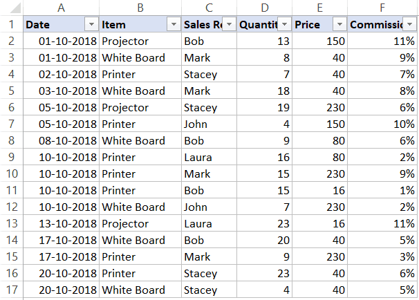
The below code would filter all the rows where the item is ‘Printer’.
Sub FilterRows()
Worksheets("Sheet1").Range("A1").AutoFilter Field:=2, Criteria1:="Printer"
End Sub
The above code refers to Sheet1 and within it, it refers to A1 (which is a cell in the dataset).
Note that here we have used Field:=2, as the item column is the second column in our dataset from the left.
Now if you’re thinking – why do I need to do this using a VBA code. This can easily be done using inbuilt filter functionality.
You’re right!
If this is all you want to do, better used the inbuilt Filter functionality.
But as you read the remaining tutorial, you’ll see that this can be combined with some extra code to create powerful automation.
But before I show you those, let me first cover a few examples to show you what all the AutoFilter method can do.
Click here to download the example file and follow along.
Example: Multiple Criteria (AND/OR) in the Same Column
Suppose I have the same dataset, and this time I want to filter all the records where the item is either ‘Printer’ or ‘Projector’.
The below code would do this:
Sub FilterRowsOR()
Worksheets("Sheet1").Range("A1").AutoFilter Field:=2, Criteria1:="Printer", Operator:=xlOr, Criteria2:="Projector"
End Sub
Note that here I have used the xlOR operator.
This tells VBA to use both the criteria and filter the data if any of the two criteria are met.
Similarly, you can also use the AND criteria.
For example, if you want to filter all the records where the quantity is more than 10 but less than 20, you can use the below code:
Sub FilterRowsAND()
Worksheets("Sheet1").Range("A1").AutoFilter Field:=4, Criteria1:=">10", _
    Operator:=xlAnd, Criteria2:="<20"
End Sub
Example: Multiple Criteria With Different Columns
Suppose you have the following dataset.
With Autofilter, you can filter multiple columns at the same time.
For example, if you want to filter all the records where the item is ‘Printer’ and the Sales Rep is ‘Mark’, you can use the below code:
Sub FilterRows()
With Worksheets("Sheet1").Range("A1")
.AutoFilter field:=2, Criteria1:="Printer"
.AutoFilter field:=3, Criteria1:="Mark"
End With
End Sub
Example: Filter Top 10 Records Using the AutoFilter Method
Suppose you have the below dataset.
Below is the code that will give you the top 10 records (based on the quantity column):
Sub FilterRowsTop10()
ActiveSheet.Range("A1").AutoFilter Field:=4, Criteria1:="10", Operator:=xlTop10Items
End Sub
In the above code, I have used ActiveSheet. You can use the sheet name if you want.
Note that in this example, if you want to get the top 5 items, just change the number in Criteria1:=”10″ from 10 to 5.
So for top 5 items, the code would be:
Sub FilterRowsTop5()
ActiveSheet.Range("A1").AutoFilter Field:=4, Criteria1:="5", Operator:=xlTop10Items
End Sub
It may look weird, but no matter how many top items you want, the Operator value always remains xlTop10Items.
Similarly, the below code would give you the bottom 10 items:
Sub FilterRowsBottom10()
ActiveSheet.Range("A1").AutoFilter Field:=4, Criteria1:="10", Operator:=xlBottom10Items
End Sub
And if you want the bottom 5 items, change the number in Criteria1:=”10″ from 10 to 5.
Example: Filter Top 10 Percent Using the AutoFilter Method
Suppose you have the same data set (as used in the previous examples).
Below is the code that will give you the top 10 percent records (based on the quantity column):
Sub FilterRowsTop10()
ActiveSheet.Range("A1").AutoFilter Field:=4, Criteria1:="10", Operator:=xlTop10Percent
End Sub
In our dataset, since we have 20 records, it will return the top 2 records (which is 10% of the total records).
Example: Using Wildcard Characters in Autofilter
Suppose you have a dataset as shown below:
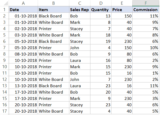
If you want to filter all the rows where the item name contains the word ‘Board’, you can use the below code:
Sub FilterRowsWildcard()
Worksheets("Sheet1").Range("A1").AutoFilter Field:=2, Criteria1:="*Board*"
End Sub
In the above code, I have used the wildcard character * (asterisk) before and after the word ‘Board’ (which is the criteria).
An asterisk can represent any number of characters. So this would filter any item that has the word ‘board’ in it.
Example: Copy Filtered Rows into a New Sheet
If you want to not only filter the records based on criteria but also copy the filtered rows, you can use the below macro.
It copies the filtered rows, adds a new worksheet, and then pastes these copied rows into the new sheet.
Sub CopyFilteredRows()
Dim rng As Range
Dim ws As Worksheet
If Worksheets("Sheet1").AutoFilterMode = False Then
MsgBox "There are no filtered rows"
Exit Sub
End If
Set rng = Worksheets("Sheet1").AutoFilter.Range
Set ws = Worksheets.Add
rng.Copy Range("A1")
End Sub
The above code would check if there are any filtered rows in Sheet1 or not.
If there are no filtered rows, it will show a message box stating that.
And if there are filtered rows, it will copy those, insert a new worksheet, and paste these rows on that newly inserted worksheet.
Example: Filter Data based on a Cell Value
Using Autofilter in VBA along with a drop-down list, you can create a functionality where as soon as you select an item from the drop-down, all the records for that item are filtered.
Something as shown below:
 Click here to download the example file and follow along.
This type of construct can be useful when you want to quickly filter data and then use it further in your work.
Below is the code that will do this:
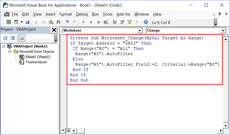
Private Sub Worksheet_Change(ByVal Target As Range)
If Target.Address = "$B$2" Then
 If Range("B2") = "All" Then
  Range("A5").AutoFilter
 Else
  Range("A5").AutoFilter Field:=2, Criteria1:=Range("B2")
 End If
End If
End Sub
This is a worksheet event code, which gets executed only when there is a change in the worksheet and the target cell is B2 (where we have the drop-down).
Also, an If Then Else condition is used to check if the user has selected ‘All’ from the drop down. If All is selected, the entire data set is shown.
This code is NOT placed in a module.
Instead, it needs to be placed in the backend of the worksheet that has this data.
Here are the steps to put this code in the worksheet code window:
- Open the VB Editor (keyboard shortcut – ALT + F11).
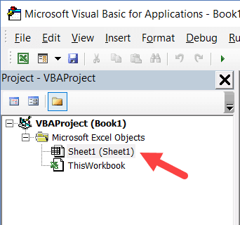
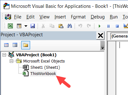
- In the Project Explorer pane, double-click on the Worksheet name in which you want this filtering functionality.

- In the worksheet code window, copy and paste the above code.

- Close the VB Editor.
Now when you use the drop-down list, it will automatically filter the data.
This is a worksheet event code, which gets executed only when there is a change in the worksheet and the target cell is B2 (where we have the drop-down).
Also, an If Then Else condition is used to check if the user has selected ‘All’ from the drop down. If All is selected, the entire data set is shown.
Turn Excel AutoFilter ON/OFF using VBA
When applying Autofilter to a range of cells, there may already be some filters in place.
You can use the below code turn off any pre-applied auto filters:
Sub TurnOFFAutoFilter()
  Worksheets("Sheet1").AutoFilterMode = False
End Sub
This code checks the entire sheets and removes any filters that have been applied.
If you don’t want to turn off filters from the entire sheet but only from a specific dataset, use the below code:
Sub TurnOFFAutoFilter()
  If Worksheets("Sheet1").Range("A1").AutoFilter Then
    Worksheets("Sheet1").Range("A1").AutoFilter
  End If
End Sub
The above code checks whether there are already filters in place or not.
If filters are already applied, it removes it, else it does nothing.
Similarly, if you want to turn on AutoFilter, use the below code:
Sub TurnOnAutoFilter()
  If Not Worksheets("Sheet1").Range("A4").AutoFilter Then
    Worksheets("Sheet1").Range("A4").AutoFilter
  End If
End Sub
Check if AutoFilter is Already Applied
If you have a sheet with multiple datasets and you want to make sure you know that there are no filters already in place, you can use the below code.
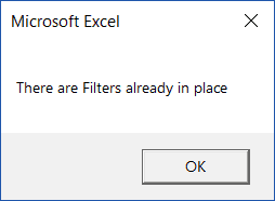
Sub CheckforFilters()
If ActiveSheet.AutoFilterMode = True Then
MsgBox "There are Filters already in place"
Else
MsgBox "There are no filters"
End If
End Sub
This code uses a message box function that displays a message ‘There are Filters already in place’ when it finds filters on the sheet, else it shows ‘There are no filters’.
Show All Data
If you have filters applied to the dataset and you want to show all the data, use the below code:
Sub ShowAllData()
If ActiveSheet.FilterMode Then ActiveSheet.ShowAllData
End Sub
The above code checks whether the FilterMode is TRUE or FALSE.
If it’s true, it means a filter has been applied and it uses the ShowAllData method to show all the data.
Note that this does not remove the filters. The filter icons are still available to be used.
Using AutoFilter on Protected Sheets
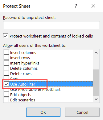
By default, when you protect a sheet, the filters won’t work.
In case you already have filters in place, you can enable AutoFilter to make sure it works even on protected sheets.
To do this, check the Use Autofilter option while protecting the sheet.
While this works when you already have filters in place, in case you try to add Autofilters using a VBA code, it won’t work.
Since the sheet is protected, it wouldn’t allow any macro to run and make changes to the Autofilter.
So you need to use a code to protect the worksheet and make sure auto filters are enabled in it.
This can be useful when you have created a dynamic filter (something I covered in the example – ‘Filter Data based on a Cell Value’).
Below is the code that will protect the sheet, but at the same time, allow you to use Filters as well as VBA macros in it.
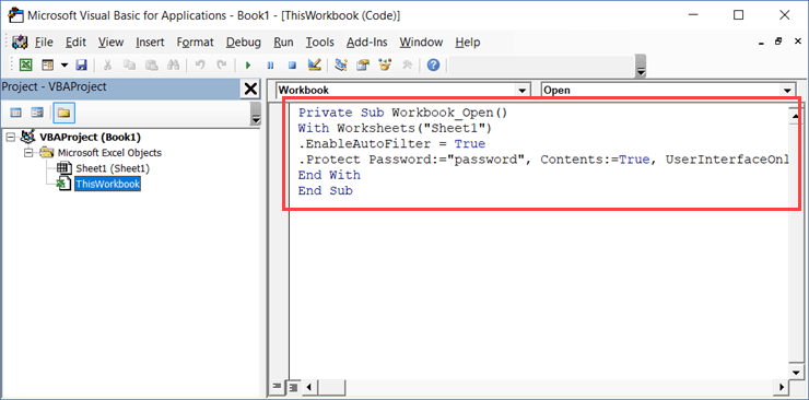
Private Sub Workbook_Open()
With Worksheets("Sheet1")
.EnableAutoFilter = True
.Protect Password:="password", Contents:=True, UserInterfaceOnly:=True
End With
End Sub
This code needs to be placed in ThisWorkbook code window.
Here are the steps to put the code in ThisWorkbook code window:
- Open the VB Editor (keyboard shortcut – ALT + F11).
- In the Project Explorer pane, double-click on the ThisWorkbook object.

- In the code window that opens, copy and paste the above code.

As soon as you open the workbook and enable macros, it will run the macro automatically and protect Sheet1.
However, before doing that, it will specify ‘EnableAutoFilter = True’, which means that the filters would work in the protected sheet as well.
Also, it sets the ‘UserInterfaceOnly’ argument to ‘True’. This means that while the worksheet is protected, the VBA macros code would continue to work.
You May Also Like the Following VBA Tutorials:
- Excel VBA Loops.
- Filter Cells with Bold Font Formatting.
- Recording a Macro.
- Sort Data Using VBA.
- Sort Worksheet Tabs in Excel.
 Excel VBA (Visual Basic for Application) is a powerful programming tool integrated with MS office suite. VBA has many constructs and methods that can be applied to manipulate data in an Excel worksheet (you can look up our introductory VBA tutorial to get a feel of all that VBA can do for you). AutoFilter in VBA is an important method that gives you the capability to filter worksheets and cells to selectively choose data.
Today, we will walk you through the AutoFilter in VBA. If you are new to VBA, we suggest that you go through our basic Excel VBA tutorial.
AutoFilter is applicable to a column or a set of columns. It filters data depending on the given criteria. The syntax of Autofilter looks like this
expression .AutoFilter(Field, Criteria1, Operator, Criteria2, VisibleDropDown)
Where
- Field- It is an integer offset of the field which contains the filter. The data type is variant, which means it can hold any data types – integers, strings, date and so on.
- Criteria1- It’s a condition based on which columns are selected.
- Operator- It specifies the type of filter. Some of the operators commonly used in Excel VBA programming are listed below.
|
Name |
Value |
Description |
|
xlAnd |
1 |
Logical AND of Criteria1 and Criteria2. |
|
xlBottom10Items |
4 |
Lowest-valued items displayed (number of items specified in Criteria1). |
|
xlBottom10Percent |
6 |
Lowest-valued items displayed (percentage specified in Criteria1). |
|
xlFilterCellColor |
8 |
Color of the cell |
|
xlFilterDynamic |
11 |
Dynamic filter |
|
xlFilterFontColor |
9 |
Color of the font |
|
xlFilterIcon |
10 |
Filter icon |
|
xlFilterValues |
7 |
Filter values |
|
xlOr |
2 |
Logical OR of Criteria1 or Criteria2. |
|
xlTop10Items |
3 |
Highest-valued items displayed (number of items specified in Criteria1). |
|
xlTop10Percent |
5 |
Highest-valued items displayed (percentage specified in Criteria1). |
- Criteria 2- This is the secondary condition based on which columns are selected. It’s combined with criteria1 and operator to create a compound criteria.
- VisibleDropDown- It’s true by default. It’s of data type variant. If it’s true then, the Autofilter dropDropDown arrow for the filtered field is displayed. If false, the dropDropDown arrow is hidden.
Now that you’re familiar with the concept and syntax of AutoFilter, lets move on to a few simple and practical exercises. Feel free to refer back to our VBA macros course at any point for more details.
Example 1: To Close All Existing AutoFilters and Create New AutoFilters
 Sub AutoFilter1()
With ActiveSheet
           .AutoFilterMode = False
           .Range("A1:E1").AutoFilter
End With
End Sub
In this program .AutoFilterMode = false turns off any existing AutoFilters. Whereas .Range(“A1:E1”).AutoFilter creates an AutoFilter which is applicable to the range A1:E1 of the active worksheet.
From here on, we will reference a worksheet which has headings in the range A1: D1 and data in the range A1:D50. The headings are as follows:
EmployeeName| E-age|Date of Joining| Department
Example 2: Using AutoFilter to match single criteria
 Sub FilterTo1Criteria()
With Sheet1
           .AutoFilterMode = False
        .Range("A1:D1").AutoFilter
           .Range("A1:D1").AutoFilter Field:=2, Criteria1:=40
End With
End Sub
This is a simple program which extracts rows where the age of the employees is 40. The “Field” value is 2 which means it refers to the second column which is ” E-age.” Criteria is that the values in column 2 should be equal to 40. Let’s take a look at the various types of criteria that you can include in your programs.
- For instances where the E-age is 40 or more, you can use the following code
Criteria1:=">=40"
- If you want to display the rows where E-age is blank, the code looks like this
Criteria1:="="
- To display all non-blanks we use
Criteria1:="<>"
- If you want to filter out the names starting with a letter “B”, in the Employee name field, then you have to assign the
Field := 1 and the Criteria1:="=B*"
- To display all names in the first column which do not contain a letter “e”, use the code
Criteria1:="<>*e*"
- If you want to hide the filter arrow then set VisibleDropDown:=False. This is the next argument after Criteria1
Example 3: Using VBA AutoFilter to Filter out Two Matching Criteria
Sub MultipleCriteria()
With Sheet1
           .AutoFilterMode = False
           .Range("A1:D1").AutoFilter
           .Range("A1:D1").AutoFilter Field:=2, Criteria1:=">=30", _
        Operator:=xlAnd, Criteria2:="<=40"
End With
 End Sub
In this program, we have specified two criteria. The operator used is the “logical And” for the 2 criteria. Thus, only those records are selected where “e-age” is “>= 30” and “<=40.”
Example 4: Using Autofilter on two different fields
Sub Filter2Fields()
With Sheet1
           .AutoFilterMode = False
               With .Range("A1:D1")
                    .AutoFilter
                    .AutoFilter Field:=1, Criteria1:="John"
                .AutoFilter Field:=4, Criteria1:="Finance"
               End With
End With
End Sub
In this program, we have selected records where Employee Name is “john” whose department is “Finance.” It is possible to add more fields; the condition being we should not exceed the total column count of headings, i.e. four.
Using Dates in AutoFilter
MS Excel uses the US date format. We recommend you to change your Date settings to this format. Else you have to use the DateSerial(). The syntax looks like this
DateSerial(year, month, day)
Let’s take a look at an example that uses the data type Date to filter columns.
Example 5: Program to Filter by Date
Sub FilterDate1()
Dim Date1 As Date
Dim str_Date As String
 Dim l_Date As Long
Date1 = DateSerial(2010, 12, 1)
l_Date = Date1
   Range("A1").AutoFilter
   Range("A1").AutoFilter Field:=1, Criteria1:=">" & l_Date
End Sub
In this program, we declare Date1 as variable of type date, str_Date as variable of type string and l_Date of variable of type long. DateSerial() function converts the date passed to it into US date format. We use Autofilter to display records more recent than the given date (1/12/2010).
Using TimeSerial Function along with VBA Autofilter
TimeSerial() function returns the time in hours, minutes and seconds. The syntax looks like this
TimeSerial(hour, minute, second)
Let’s take a close look at the parameters to understand them better. All the three parameters require integer data type.
- Hour: any number between 0 and 23 inclusive or a numeric expression.
- Minute: any numeric expression.
- Second: any numeric expression.
TimeSerial(17, 28, 20) will return the serial representation of 5: 28:20 PM. TimeSerial() can be used along with the DateSerial() to return the exact time and date in a VBA program.
Example 5: Using Autofilter to Filter by Date and Time
 Sub FilterDateTime()
Dim d_Date As Date
Dim db_Date As Double
If IsDate(Range("B1")) Then
   db_Date = Range("B1")
db_Date = DateSerial(Year(db_Date), Month(db_Date), Day(db_Date)) + _
        TimeSerial(Hour(db_Date), Minute(db_Date), Second(db_Date))
   Range("A1").AutoFilter
    Range("A1").AutoFilter Field:=1, Criteria1:=">" & db_Date
End If
End Sub
In this program IsDate() is used to see whether the cell contains an expression that can be converted into a date. Then the content of the cell is assigned to the db_Date variable. Next DateSerial() and TimeSerail () are combined and the result assigned to db_Date. We filter the records using Field 1 as criteria to return dates greater than db_Date.
Excel VBA is an exciting programming area. It equips you with features and functionalities to develop simple and efficient code. AutoFilter is central to Excel VBA programming. Leverage it to provide different views of the data. MrExcel shows some neat tricks in this VBA course, that can help you out. Once you’re ready to tackle more advanced usage, you can do so with our Ultimate VBA course.
Содержание
- Объект AutoFilter (Excel)
- Пример
- Методы
- Свойства
- См. также
- Поддержка и обратная связь
- Range.AutoFilter method (Excel)
- Syntax
- Parameters
- Return value
- Remarks
- Example
- Support and feedback
- Vba excel включить фильтры
Объект AutoFilter (Excel)
Представляет автофильтровку для указанного листа.
При использовании автофильтра с датами формат должен соответствовать разделителям дат на английском языке («/») вместо локальных параметров («.»). Допустимая дата будет «2/2/2/2007», тогда как «2.2.2007» является недопустимой.
Для работы с объектами (например, объектом Interior ) требуется добавить ссылку на объект . Дополнительные сведения о назначении ссылки на объект переменной или свойству см. в инструкции Set .
Пример
Используйте свойство AutoFilter объекта Worksheet , чтобы вернуть объект AutoFilter . Используйте свойство Filters для возврата коллекции отдельных фильтров столбцов. Используйте свойство Range , чтобы вернуть объект Range , представляющий весь отфильтрованный диапазон.
В следующем примере сохраняются критерии адреса и фильтрации для текущей фильтрации, а затем применяются новые фильтры.
Чтобы создать объект AutoFilter для листа, необходимо включить автоматическое фильтрацию для диапазона на листе вручную или с помощью метода AutoFilter объекта Range . В следующем примере используются значения, хранящиеся в переменных уровня модуля в предыдущем примере, для восстановления исходной автофильтрации на листе Crew.
Методы
Свойства
См. также
Поддержка и обратная связь
Есть вопросы или отзывы, касающиеся Office VBA или этой статьи? Руководство по другим способам получения поддержки и отправки отзывов см. в статье Поддержка Office VBA и обратная связь.
Источник
Range.AutoFilter method (Excel)
Filters a list by using the AutoFilter.
Syntax
expression.AutoFilter (Field, Criteria1, Operator, Criteria2, SubField, VisibleDropDown)
expression An expression that returns a Range object.
Parameters
| Name | Required/Optional | Data type | Description |
|---|---|---|---|
| Field | Optional | Variant | The integer offset of the field on which you want to base the filter (from the left of the list; the leftmost field is field one). |
| Criteria1 | Optional | Variant | The criteria (a string; for example, «101»). Use «=» to find blank fields, «<>» to find non-blank fields, and «> to select (No Data) fields in data types. |
If this argument is omitted, the criteria is All. If Operator is xlTop10Items, Criteria1 specifies the number of items (for example, «10»). Operator Optional XlAutoFilterOperator An XlAutoFilterOperator constant specifying the type of filter. Criteria2 Optional Variant The second criteria (a string). Used with Criteria1 and Operator to construct compound criteria. Also used as single criteria on date fields filtering by date, month or year. Followed by an Array detailing the filtering Array(Level, Date). Where Level is 0-2 (year,month,date) and Date is one valid Date inside the filtering period. SubField Optional Variant The field from a data type on which to apply the criteria (for example, the «Population» field from Geography or «Volume» field from Stocks). Omitting this value targets the «(Display Value)». VisibleDropDown Optional Variant True to display the AutoFilter drop-down arrow for the filtered field. False to hide the AutoFilter drop-down arrow for the filtered field. True by default.
Return value
If you omit all the arguments, this method simply toggles the display of the AutoFilter drop-down arrows in the specified range.
Excel for Mac does not support this method. Similar methods on Selection and ListObject are supported.
Unlike in formulas, subfields don’t require brackets to include spaces.
Example
This example filters a list starting in cell A1 on Sheet1 to display only the entries in which field one is equal to the string Otis. The drop-down arrow for field one will be hidden.
This example filters a list starting in cell A1 on Sheet1 to display only the entries in which the values of field one contain a SubField, Admin Division 1 (State/province/other), where the value is Washington.
This example filters a table, Table1, on Sheet1 to display only the entries in which the values of field one have a «(Display Value)» that is either 1, 3, Seattle, or Redmond.
Data types can apply multiple SubField filters. This example filters a table, Table1, on Sheet1 to display only the entries in which the values of field one contain a SubField, Time Zone(s), where the value is Pacific Time Zone, and where the SubField named Date Founded is either 1851 or there is «(No Data)».
This example filters a table, Table1, on Sheet1 to display the Top 10 entries for field one based off the Population SubField.
This example filters a table, Table1, on Sheet1 to display the all entries for January 2019 and February 2019 for field one. There does not have to be a row containing January the 31.
Support and feedback
Have questions or feedback about Office VBA or this documentation? Please see Office VBA support and feedback for guidance about the ways you can receive support and provide feedback.
Источник
Vba excel включить фильтры

Ф ильтры на VBA (AutoFilter Method): самое подробное руководство в рунете
Автор Дмитрий Якушев На чтение11 мин. Просмотров2.6k.
Итог: научиться создавать макросы, использовать фильтры на диапазоны и таблицы с помощью метода AutoFilter VBA. Статья содержит ссылки на примеры для фильтрации различных типов данных, включая текст, цифры, даты, цвета и значки.
Уровень мастерства: средний
- Скачать файл
- Написание макросов для фильтров
- Макро-рекордер — твой друг (или враг)
- Метод автофильтрации
- Написание кода автофильтра
- Шаг 1: Ссылка на диапазон или таблицу
- Диапазоны или таблицы?
- 5 (или 6) параметров автофильтра
- Шаг 2: Параметр поля
- Шаг 3: Параметры критериев
- Общие правила дляCriteria1 и Criteria2
- Шаг 4: Параметр оператора
- Автофильтр не является дополнением
- Как установить номер поля динамически
- Используйте таблицы Excel с фильтрами
- Фильтры и типы данных
- Почему метод автофильтрации такой сложный?
Файл Excel, содержащий код, можно скачать ниже. Этот файл содержит код для фильтрации различных типов данных и типов фильтров.
VBA AutoFilters Guide.xlsm (100.5 KB)
Н аписание макросов для фильтров
Фильтры являются отличным инструментом для анализа данных в Excel. Для большинства аналитиков и частых пользователей Excel фильтры являются частью нашей повседневной жизни. Мы используем раскрывающиеся меню фильтров для применения фильтров к отдельным столбцам в наборе данных. Это помогает нам связывать цифры с отчетами и проводить исследование наших данных.
Фильтрация также может быть трудоемким процессом. Особенно, когда мы применяем фильтры к нескольким столбцам на больших листах или фильтруем данные, чтобы затем копировать / вставлять их в другие листы или книги.
В этой статье объясняется, как создавать макросы для автоматизации процесса фильтрации. Это обширное руководство по методу автофильтра в VBA.
У меня также есть статьи с примерами для различных фильтров и типов данных, в том числе: пробелы, текст, числа, даты, цвета и значки, и очищающие фильтры.
М акро-рекордер — твой друг (или враг)
Мы можем легко получить код VBA для фильтров, включив макро-рекордер, а затем применив один или несколько фильтров к диапазону / таблице.
Вот шаги для создания макроса фильтра с помощью устройства записи макросов:
- Включите рекордер макросов:
- Вкладка «Разработчик»> «Запись макроса».
- Дайте макросу имя, выберите, где вы хотите сохранить код, и нажмите ОК.
- Примените один или несколько фильтров, используя раскрывающиеся меню фильтров.
- Остановите рекордер.
- Откройте редактор VB (вкладка «Разработчик»> Visual Basic) для просмотра кода.
Если вы уже использовали макрос-рекордер для этого процесса, то вы знаете, насколько он может быть полезен. Тем более, что наши критерии фильтрации становятся более сложными.
Код будет выглядеть примерно так:
ActiveSheet.ListObjects(«tblData»).Range.AutoFilter Field:=4, Criteria1:= _
ActiveSheet.ListObjects(«tblData»).Range.AutoFilter Field:=5, Criteria1:= _
«>=500″, Operator:=xlAnd, Criteria2:=»
Мы видим, что каждая строка использует метод AutoFilter для применения фильтра к столбцу. Он также содержит информацию о критериях фильтра.
Мы видим, что каждая строка использует метод AutoFilter для применения фильтра к столбцу. Он также содержит информацию о критериях фильтра.
М етод автофильтрации
Метод AutoFilter используется для очистки и применения фильтров к одному столбцу в диапазоне или таблице в VBA. Он автоматизирует процесс применения фильтров через выпадающие меню фильтров и делает, чтобы все работало. 
Его можно использовать для применения фильтров к нескольким столбцам путем написания нескольких строк кода, по одной для каждого столбца. Мы также можем использовать Автофильтр, чтобы применить несколько критериев фильтрации к одному столбцу, так же, как в выпадающем меню фильтра, установив несколько флажков или указав диапазон дат.
Н аписание кода автофильтра
Вот пошаговые инструкции по написанию строки кода для автофильтра.
Ш аг 1: Ссылка на диапазон или таблицу
Метод AutoFilter является частью объекта Range. Поэтому мы должны ссылаться на диапазон или таблицу, к которым применяются фильтры на листе. Это будет весь диапазон, к которому применяются фильтры.
Следующие примеры включают / отключают фильтры в диапазоне B3: G1000 на листе автофильтра.
‘Автофильтр является членом объекта Range
‘Ссылка на весь диапазон, к которому применяются фильтры
‘Автофильтр включает / выключает фильтры, когда параметры не указаны.
‘Полностью квалифицированный справочник, начиная с уровня Workbook
Вот пример использования таблиц Excel.
‘Автофильтры на таблицах работают одинаково.
Dim lo As ListObject ‘Excel Table
‘Установить переменную ListObject (Table)
Set lo = Sheet1.ListObjects(1)
‘Автофильтр является членом объекта Range
‘Родителем объекта Range является объект List
Метод AutoFilter имеет 5 необязательных параметров, которые мы рассмотрим далее. Если мы не укажем ни один из параметров, как в приведенных выше примерах, метод AutoFilter включит / выключит фильтры для указанного диапазона. Это переключение. Если фильтры включены, они будут выключены, и наоборот.
Д иапазоны или таблицы?
Фильтры работают одинаково как для обычных диапазонов , так и для таблиц Excel . 
Я отдаю предпочтение методу использования таблиц, потому что нам не нужно беспокоиться об изменении ссылок на диапазон при увеличении или уменьшении таблицы. Однако код будет одинаковым для обоих объектов. В остальных примерах кода используются таблицы Excel, но вы можете легко изменить это для обычных диапазонов.
5 (или 6) параметров автофильтра
Метод AutoFilter имеет 5 (или 6) необязательных параметров, которые используются для указания критериев фильтрации для столбца. Вот список параметров. 

Страница справки MSDN
Мы можем использовать комбинацию этих параметров, чтобы применять различные критерии фильтрации для разных типов данных. Первые четыре являются наиболее важными, поэтому давайте посмотрим, как их применять.
Ш аг 2: Параметр поля
Первый параметр — это Field. Для параметра Field мы указываем число, которое является номером столбца, к которому будет применяться фильтр. Это номер столбца в диапазоне фильтра, который является родителем метода AutoFilter. Это НЕ номер столбца на рабочем листе.
В приведенном ниже примере поле 4 является столбцом «Продукт», поскольку это 4-й столбец в диапазоне фильтра / таблице. 
Фильтр столбца очищается, когда мы указываем только параметр Field, а другие критерии отсутствуют. 
Мы также можем использовать переменную для параметра Field и установить ее динамически. Я объясню это более подробно ниже.
Ш аг 3: Параметры критериев
Существует два параметра, которые можно использовать для указания фильтра Критерии, Criteria1 и Criteria2 . Мы используем комбинацию этих параметров и параметра Operator для разных типов фильтров. Здесь все становится сложнее, поэтому давайте начнем с простого примера.
‘Фильтровать столбец «Продукт» для одного элемента
lo.Range.AutoFilter Field:=4, Criteria1:=»Product 2″
Это то же самое, что выбрать один элемент из списка флажков в раскрывающемся меню фильтра. 
О бщие правила для Criteria1 и Criteria2
Значения, которые мы указываем для Criteria1 и Criteria2, могут быть хитрыми. Вот несколько общих рекомендаций о том, как ссылаться на значения параметра Criteria.
- Значением критерия является строка, заключенная в кавычки. Есть несколько исключений, когда критерии являются постоянными для периода времени даты и выше / ниже среднего.
- При указании фильтров для отдельных чисел или дат форматирование чисел должно соответствовать форматированию чисел, применяемому в диапазоне / таблице.
- Оператор сравнения больше / меньше чем также включен в кавычки перед числом.
- Кавычки также используются для фильтров для пробелов «=» и не пробелов «<>».
‘Фильтр на дату, большую или равную 1 января 2015 г.
lo.Range.AutoFilter Field:=1, Criteria1:=»>=1/1/2015″
‘ Оператор сравнения> = находится внутри кавычек
‘ для параметра Criteria1.
‘ Форматирование даты в коде соответствует форматированию
‘ применяется к ячейкам на листе.
Ш аг 4: Параметр оператора
Что если мы хотим выбрать несколько элементов из раскрывающегося списка фильтров? Или сделать фильтр для диапазона дат или чисел?
Для этого нам нужен Operator . Параметр Operator используется для указания типа фильтра, который мы хотим применить. Он может варьироваться в зависимости от типа данных в столбце. Для
Operator должна использоваться одна из следующих 11 констант. 
Вот ссылка на страницу справки MSDN, которая содержит список констант для перечисления XlAutoFilterOperator .
Operator используется в сочетании с Criteria1 и / или Criteria2, в зависимости от типа данных и типа фильтра. Вот несколько примеров.
‘Фильтр для списка нескольких элементов, оператор — xlFilterValues
Criteria1:=Array(«Product 4», «Product 5», «Product 6»), _
‘Фильтр для диапазона дат (между датами), оператор xlAnd
Это основы написания строки кода для метода AutoFilter. Будет сложнее с различными типами данных.
Итак, я привел много примеров ниже, которые содержат большинство комбинаций критериев и операторов для разных типов фильтров.
А втофильтр не является дополнением
При запуске строки кода автофильтра сначала удаляются все фильтры, примененные к этому столбцу (полю), а затем применяются критерии фильтра, указанные в строке кода.
Это означает, что это не дополнение. Следующие 2 строки НЕ создадут фильтр для Продукта 1 и Продукта 2. После запуска макроса столбец Продукт будет отфильтрован только для Продукта 2.
‘Автофильтр НЕ ДОБАВЛЯЕТ. Это сначала любые фильтры, применяемые
‘в столбце перед применением нового фильтра
lo.Range.AutoFilter Field:=4, Criteria1:=»Product 3″
‘Эта строка кода отфильтрует столбец только для продукта 2
‘Фильтр для Продукта 3 выше будет очищен при запуске этой линии.
lo.Range.AutoFilter Field:=4, Criteria1:=»Product 2″
Если вы хотите применить фильтр с несколькими критериями к одному столбцу, вы можете указать это с помощью параметров
Criteria и Operator .
К ак установить номер поля динамически
Если мы добавим / удалим / переместим столбцы в диапазоне фильтра, то номер поля для отфильтрованного столбца может измениться. Поэтому я стараюсь по возможности избегать жесткого кодирования числа для параметра Field.
Вместо этого мы можем использовать переменную и использовать некоторый код, чтобы найти номер столбца по его имени. Вот два примера для обычных диапазонов и таблиц. 
‘Методы, чтобы найти и установить поле на основе имени столбца.
Dim lo As ListObject
Dim iCol As Long
‘Установить ссылку на первую таблицу на листе
Set lo = Sheet1.ListObjects(1)
‘Установить поле фильтра
‘Использовать функцию соответствия для регулярных диапазонов
‘iCol = WorksheetFunction.Match(«Product», Sheet1.Range(«B3:G3»), 0)
‘Использовать переменную для значения параметра поля
lo.Range.AutoFilter Field:=iCol, Criteria1:=»Product 3″
Номер столбца будет найден при каждом запуске макроса. Нам не нужно беспокоиться об изменении номера поля при перемещении столбца. Это экономит время и предотвращает ошибки (беспроигрышный вариант)!
И спользуйте таблицы Excel с фильтрами
Использование таблиц Excel дает множество преимуществ, особенно при использовании метода автофильтрации. Вот несколько основных причин, по которым я предпочитаю таблицы.
- Нам не нужно переопределять диапазон в VBA, поскольку диапазон данных изменяет размер (строки / столбцы добавляются / удаляются). На всю таблицу ссылается объект ListObject.
- Данные в таблице легко ссылаться после применения фильтров. Мы можем использовать свойство DataBodyRange для ссылки на видимые строки для копирования / вставки, форматирования, изменения значений и т.д.
- Мы можем иметь несколько таблиц на одном листе и, следовательно, несколько диапазонов фильтров. С обычными диапазонами у нас может быть только один отфильтрованный диапазон на лист.
- Код для очистки всех фильтров в таблице легче написать.
Ф ильтры и типы данных
Параметры раскрывающегося меню фильтра изменяются в зависимости от типа данных в столбце. У нас есть разные фильтры для текста, чисел, дат и цветов. Это создает МНОГО различных комбинаций операторов и критериев для каждого типа фильтра.
Я создал отдельные посты для каждого из этих типов фильтров. Посты содержат пояснения и примеры кода VBA.
- Как очистить фильтры с помощью VBA
- Как отфильтровать пустые и непустые клетки
- Как фильтровать текст с помощью VBA
- Как фильтровать числа с помощью VBA
- Как отфильтровать даты с помощью VBA
- Как отфильтровать цвета и значки с помощью VBA
Файл в разделе загрузок выше содержит все эти примеры кода в одном месте. Вы можете добавить его в свою личную книгу макросов и использовать макросы в своих проектах.
П очему метод автофильтрации такой сложный?
Этот пост был вдохновлен вопросом от Криса, участника The VBA Pro Course. Комбинации Критерии и Операторы могут быть запутанными и сложными. Почему это?
Ну, фильтры развивались на протяжении многих лет. Мы увидели много новых типов фильтров, представленных в Excel 2010, и эта функция продолжает улучшаться. Однако параметры метода автофильтра не изменились. Они отлично подходят для совместимости со старыми версиями, но также означает, что новые типы фильтров работают с существующими параметрами.
Большая часть кода фильтра имеет смысл, но сначала может быть сложно разобраться. К счастью, у нас есть макро рекордер, чтобы помочь с этим.
Я надеюсь, что вы можете использовать эту статью и файл Excel в качестве руководства по написанию макросов для фильтров. Автоматизация фильтров может сэкономить нам и нашим пользователям массу времени, особенно при использовании этих методов в более крупном проекте автоматизации данных.
Источник