
Вырезание, перемещение, копирование и вставка ячеек (диапазонов) в VBA Excel. Методы Cut, Copy и PasteSpecial объекта Range, метод Paste объекта Worksheet.
Метод Range.Cut
Range.Cut – это метод, который вырезает объект Range (диапазон ячеек) в буфер обмена или перемещает его в указанное место на рабочем листе.
Синтаксис
Параметры
| Параметры | Описание |
|---|---|
| Destination | Необязательный параметр. Диапазон ячеек рабочего листа, в который будет вставлен (перемещен) вырезанный объект Range (достаточно указать верхнюю левую ячейку диапазона). Если этот параметр опущен, объект вырезается в буфер обмена. |
Для вставки на рабочий лист диапазона ячеек, вырезанного в буфер обмена методом Range.Cut, следует использовать метод Worksheet.Paste.
Метод Range.Copy
Range.Copy – это метод, который копирует объект Range (диапазон ячеек) в буфер обмена или в указанное место на рабочем листе.
Синтаксис
Параметры
| Параметры | Описание |
|---|---|
| Destination | Необязательный параметр. Диапазон ячеек рабочего листа, в который будет вставлен скопированный объект Range (достаточно указать верхнюю левую ячейку диапазона). Если этот параметр опущен, объект копируется в буфер обмена. |
Метод Worksheet.Paste
Worksheet.Paste – это метод, который вставляет содержимое буфера обмена на рабочий лист.
Синтаксис
|
Worksheet.Paste (Destination, Link) |
Метод Worksheet.Paste работает как с диапазонами ячеек, вырезанными в буфер обмена методом Range.Cut, так и скопированными в буфер обмена методом Range.Copy.
Параметры
| Параметры | Описание |
|---|---|
| Destination | Необязательный параметр. Диапазон (ячейка), указывающий место вставки содержимого буфера обмена. Если этот параметр не указан, используется текущий выделенный объект. |
| Link | Необязательный параметр. Булево значение, которое указывает, устанавливать ли ссылку на источник вставленных данных: True – устанавливать, False – не устанавливать (значение по умолчанию). |
В выражении с методом Worksheet.Paste можно указать только один из параметров: или Destination, или Link.
Для вставки из буфера обмена отдельных компонентов скопированных ячеек (значения, форматы, примечания и т.д.), а также для проведения транспонирования и вычислений, используйте метод Range.PasteSpecial (специальная вставка).
Примеры
Вырезание и вставка диапазона одной строкой (перемещение):
|
Range(«A1:C3»).Cut Range(«E1») |
Вырезание ячеек в буфер обмена и вставка методом ActiveSheet.Paste:
|
Range(«A1:C3»).Cut ActiveSheet.Paste Range(«E1») |
Копирование и вставка диапазона одной строкой:
|
Range(«A18:C20»).Copy Range(«E18») |
Копирование ячеек в буфер обмена и вставка методом ActiveSheet.Paste:
|
Range(«A18:C20»).Copy ActiveSheet.Paste Range(«E18») |
Копирование одной ячейки и вставка ее данных во все ячейки заданного диапазона:
|
Range(«A1»).Copy Range(«B1:D10») |
Home / VBA / VBA Copy Range to Another Sheet + Workbook
To copy a cell or a range of cells to another worksheet you need to use the VBA’s “Copy” method. In this method, you need to define the range or the cell using the range object that you wish to copy and then define another worksheet along with the range where you want to paste it.
Copy a Cell or Range to Another Worksheet
Range("A1").Copy Worksheets("Sheet2").Range("A1")- First, define the range or the cell that you want to copy.

- Next, type a dot (.) and select the copy method from the list of properties and methods.

- Here you’ll get an intellisense to define the destination of the cell copied.

- From here, you need to define the worksheet and then the destination range.


Now when you run this code, it will copy cell A1 from the active sheet to the “Sheet2”. There’s one thing that you need to take care that when you copy a cell and paste it to a destination it also pastes the formatting there.
But if you simply want to copy the value from a cell and paste it into the different worksheets, consider the following code.
Worksheets("Sheet2").Range("A1") = Range("A1").ValueThis method doesn’t use the copy method but simply adds value to the destination worksheet using an equal sign and using the value property with the source cell.
Copy Cell from a Different Worksheet
Now let’s say you want to copy a cell from a worksheet that is not active at the time. In this case, you need to define the worksheet with the source cell. Just like the following code.
Worksheets("sheet1").Range("A1").Copy Worksheets("Sheet2").Range("A1")Copy a Range of Cells
Range("A1:A10").Copy Worksheets("Sheet2").Range("A1:A10")
Range("A1:A10").Copy Worksheets("Sheet2").Range("A1")
Copy a Cell to a Worksheet in Another Workbook
When workbooks are open but not saved yet.
Workbooks("Book1").Worksheets("Sheet1").Range("A1").Copy _
Workbooks("Book2").Worksheets("Sheet1").Range("A1")
When workbooks are open and saved.
Workbooks("Book1.xlsx").Worksheets("Sheet1").Range("A1").Copy _
Workbooks("Book2.xlsx").Worksheets("Sheet1").Range("A1")
Copy a Cell to a Worksheet in Another Workbook which is Closed
'to open the workbook that is saved in a folder on your system _
change the path according to the location you have in your _
system
Workbooks.Open "C:UsersDellDesktopmyFile.xlsx"

'copies cell from the book1 workbook and copy and paste _
it to the workbook myFile
Workbooks("Book1").Worksheets("Sheet1").Range("A1").Copy _
Workbooks("myFile").Worksheets("Sheet1").Range("A1")

'close the workbook and after saving
Workbooks("myFile").Close SaveChanges:=True
Related: How to Open a Workbook using VBA in Excel
More Tutorials
- Count Rows using VBA in Excel
- Excel VBA Font (Color, Size, Type, and Bold)
- Excel VBA Hide and Unhide a Column or a Row
- Excel VBA Range – Working with Range and Cells in VBA
- Apply Borders on a Cell using VBA in Excel
- Find Last Row, Column, and Cell using VBA in Excel
- Insert a Row using VBA in Excel
- Merge Cells in Excel using a VBA Code
- Select a Range/Cell using VBA in Excel
- SELECT ALL the Cells in a Worksheet using a VBA Code
- ActiveCell in VBA in Excel
- Special Cells Method in VBA in Excel
- UsedRange Property in VBA in Excel
- VBA AutoFit (Rows, Column, or the Entire Worksheet)
- VBA ClearContents (from a Cell, Range, or Entire Worksheet)
- VBA Enter Value in a Cell (Set, Get and Change)
- VBA Insert Column (Single and Multiple)
- VBA Named Range | (Static + from Selection + Dynamic)
- VBA Range Offset
- VBA Sort Range | (Descending, Multiple Columns, Sort Orientation
- VBA Wrap Text (Cell, Range, and Entire Worksheet)
- VBA Check IF a Cell is Empty + Multiple Cells
⇠ Back to What is VBA in Excel
Helpful Links – Developer Tab – Visual Basic Editor – Run a Macro – Personal Macro Workbook – Excel Macro Recorder – VBA Interview Questions – VBA Codes
Настоящая заметка продолжает знакомство с VBA, в ней описана работа с диапазонами в VBA.[1]
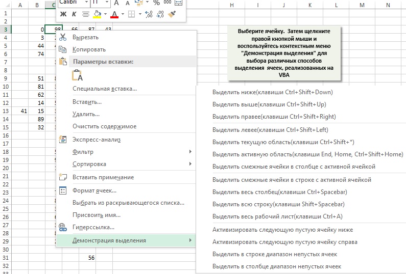
Рис. 1. Пример, демонстрирующий, как выделять диапазоны различной формы в VBA$ чтобы увеличить изображение кликните на нем правой кнопкой мыши и выберите Открыть картинку в новой вкладке
Скачать заметку в формате Word или pdf, примеры в архиве (политика безопасности провайдера не позволяет загружать файлы Excel с поддержкой макросов)
Копирование диапазона
Функция записи макросов Excel используется не столько для создания хорошего кода, сколько для поиска названий необходимых объектов, методов и свойств. Например, при записи операции копирования и вставки можно получить код:
Sub Макрос()
Range("A1").Select
Selection.Copy
Range("B1").Select
ActiveSheet.Paste
End Sub
Обратите внимание, что данная программа выделяет ячейки. Однако в VBA для работы с объектом не обязательно его выделять. Данную процедуру можно заменить значительно более простой — применить метод Сору, который использует аргумент, представляющий адрес места вставки копируемого диапазона.
Sub CopyRange()
Range("А1").Copy Range("В1")
End Sub
Предполагается, что рабочий лист является активным и операция выполняется на активном рабочем листе. Чтобы скопировать диапазон на другой рабочий лист или в другую книгу, необходимо задать ссылку:
Sub CopyRange2()
Workbooks("File1.xlsx").Sheets("Лист1").Range("A1").Copy _
Workbooks("File2.xlsx").Sheets("Лист2").Range("A1")
End Sub
Еще одним подходом к решению этой задачи является использование для представления диапазонов объектных переменных:
Sub CopyRange3()
Dim Rngl As Range, Rng2 As Range
Set Rngl = Workbooks("File1.xlsx").Sheets("Лист1").Range("A1")
Set Rng2 = Workbooks("File2.xlsx").Sheets("Лист2").Range("A1")
Rngl.Copy Rng2 End Sub
Можно копировать большой диапазон. Адрес места вставки определяется единственной ячейкой (представляющей верхний левый угол вставляемого диапазона):
Sub CopyRange4 ()
Range("А1:С800").Copy Range("D1")
End Sub
Для перемещения диапазона ячеек вместо метода Сору используется метод Cut.
Если размер копируемого диапазона не известен используется свойство CurrentRegion, возвращающее объект Range, который соответствует прямоугольнику ячеек вокруг заданной ячейки:
Sub CopyCurrentRegion2()
Range("A1").CurrentRegion.Copy Sheets("Лист2").Range("A1")
End Sub
Метод End имеет один аргумент, определяющий направление, в котором увеличивается выделение ячеек. Следующий оператор выделяет диапазон от активной ячейки до последней непустой ячейки внизу:
Range (ActiveCell, ActiveCell.End(xlDown)).Select
Три остальные константы имитируют комбинации клавиш при выделении в других направлениях: xlUp (вверх), xlToLeft (влево) и xlToRight (вправо).
В прилагаемом Excel-файле определено несколько распространенных типов выделения ячеек (см. рис. 1). Код любопытен тем, что является также примером создания контекстного меню.
Запрос значения ячейки
Следующая процедура запрашивает значение у пользователя и вставляет его в ячейку А1:
Sub GetValuel()
Range("A1").Value = InputBox("Введите значение")
End Sub
Однако при выполнении этой процедуры возникает проблема. Если пользователь щелкнет на кнопке Отмена в окне ввода данных, то процедура удалит данные, которые находились в текущей ячейке. Модифицированная версия процедуры адекватно реагирует на щелчок на кнопке Отмена и не выполняет при этом никаких действий:
Sub GetValue2()
Dim UserEntry As Variant
UserEntry = InputBox("Введите значение")
If UserEntry <> "" Then Range("A1").Value = UserEntry
End Sub
Во многих случаях следует проверить правильность данных, введенных пользователем. Например, необходимо обеспечить введение только чисел в диапазоне от 1 до 12 (рис. 2). Это можно сделать при помощи процедуры GetValue3(), код которой приведен в Модуле1 приложенного Excel-файла. Некорректные данные игнорируются, и окно запроса значения отображается снова. Этот цикл будет повторяться, пока пользователь не введет правильное значение или не щелкнет на кнопке Отмена.

Рис. 2. Проверка данных, введенных пользователем
Ввод значения в следующую пустую ячейку
Если требуется ввести значение в следующую пустую ячейку столбца или строки, используйте код (рис. 3):
Sub GetData()
Dim NextRow As Long
Dim Entry1 As String, Entry2 As String
Do
' Определение следующей пустой строки
NextRow = Cells(Rows.Count, 1).End(xlUp).Row + 1
' Запрос данных
Entry1 = InputBox("Введите имя")
If Entry1 = "" Then Exit Sub
Entry2 = InputBox("Введите сумму")
If Entry2 = "" Then Exit Sub
' Запись данных
Cells(NextRow, 1) = Entry1
Cells(NextRow, 2) = Entry2
Loop
End Sub

Рис. 3. Макрос вставляет данные в следующую пустую строку рабочего листа
Это бесконечный цикл. Для выхода из него (щелкните на кнопке Cancel) использовались операторы Exit Sub. Обратите внимание строку, в который определяется значение переменной NextRow. Если вам трудно ее понять, проанализируйте содержимое ячейки: перейдите в последнюю ячейку столбца А и нажмите <End> и <↑>. После этого будет выделена последняя непустая ячейка в столбце А. Свойство Row возвращает номер этой строки; чтобы получить расположенную под ней строку (следующую пустую строку), к этому номеру прибавляется 1.
Приостановка работы макроса для определения диапазона пользователем
В некоторых ситуациях макрос должен взаимодействовать с пользователем. Например, можно создать макрос, который приостанавливается, когда пользователь указывает диапазон ячеек. Для этого воспользуйтесь функцией Excel InputBox. Не путайте метод Excel InputBox с функцией VBA InputBox. Несмотря на идентичность названий, это далеко не одно и то же.
Процедура, представленная ниже, демонстрирует, как приостановить макрос и разрешить пользователю выбрать ячейку. Затем автоматически формула вставляется в каждую ячейку выделенного диапазона.
Sub GetUserRange()
Dim UserRange As Range
Prompt = "Выберите диапазон для случайных чисел."
Title = "Выбор диапазона"
' Отображение поля ввода
On Error Resume Next
Set UserRange = Application.InputBox( _
Prompt:=Prompt, _
Title:=Title, _
Default:=ActiveCell.Address, _
Type:=8) 'Выделение диапазона
On Error GoTo 0
' Отменено ли отображение поля ввода?
If UserRange Is Nothing Then
MsgBox "Отменено."
Else
UserRange.Formula = "=RAND()"
End If
End Sub
Окно ввода данных показано на рис. 4. Важный момент в этой процедуре – определение аргумента Туре равным 8 (в этом случае InputBox вернет диапазон; подробнее см. Application.InputBox Method).

Рис. 4. Использование окна ввода данных с целью приостановки выполнения макроса
Оператор On Error Resume Next игнорирует ошибку, если пользователь не выберет диапазон, а щелкает Отмена. В таком случае объектная переменная UserRange не получает значения. В этом случае отобразится окно сообщения с текстом «Отменено». Если же пользователь щелкнет на кнопке OK, то макрос продолжит выполняться. Строка On Error Go То указывает на переход к стандартной обработке ошибки. Проверка корректного выделения диапазона необязательна. Excel позаботится об этом вместо вас.
Обязательно проверьте, включено ли обновление экрана при использовании метода InputBox для выделения диапазона. Если обновление экрана отключено, вы не сможете выделить рабочий лист. Чтобы проконтролировать обновление экрана, в процессе выполнения макроса используйте свойство ScreenUpdating объекта Application.
Подсчет выделенных ячеек
Работая с макросом, который обрабатывает выделенный диапазон ячеек, можно использовать свойство Count, чтобы определить, сколько ячеек содержится в выделенном (или любом другом) диапазоне. Например, оператор MsgBox Selection.Count демонстрирует окно сообщения, которое отображает количество ячеек в текущем выделенном диапазоне. Свойство Count использует тип данных Long, поэтому наибольшее значение, которое может храниться в нем, равно 2 147 483 647. Если выделить лист целиком, то ячеек будет больше, и свойство Count сгенерирует ошибку. Используйте свойство CountLarge, которое не имеет таких ограничений.
Если активный лист содержит диапазон data, то следующий оператор присваивает количество ячеек в диапазоне data переменной с названием CellCount:
CellCount = Range("data").Count
Вы можете также определить, сколько строк или столбцов содержится в диапазоне. Следующее выражение вычисляет количество столбцов в выделенном диапазоне:
Selection.Columns.Count
Следующий оператор пересчитывает количество строк в диапазоне с названием data и присваивает это количество переменной RowCount.
RowCount = Range("data").Rows.Count
Просмотр выделенного диапазона
Вы можете столкнуться с трудностями при создании макроса, который оценивает каждую ячейку в диапазоне и выполняет операцию, определенную заданному критерию. Если выделен целый столбец или строка, то работа макроса может занять много времени. Процедура ColorNegative устанавливает красный цвет для ячеек, которые содержат отрицательные значения. Цвет фона для других ячеек не определяется. Код процедуры можно найти в Модуле4 приложенного Excel-файла.
Усовершенствованная процедура ColorNegative2, создает объектную переменную WorkRange типа Range, которая представляет собой пересечение выделенного диапазона и диапазона рабочего листа (рис. 5). Если выделить столбец F (1048576 ячеек), то его пересечение с рабочим диапазоном В2:I16) даст область F2:F16, которая намного меньше исходного выделенного диапазона. Время, затрачиваемое на обработку 15 ячеек, намного меньше времени, уходящего на обработку миллиона ячеек.

Рис. 5. В результате пересечения используемого диапазона и выделенного диапазона рабочего листа уменьшается количество обрабатываемых ячеек
И всё же процедура ColorNegative2 недостаточно эффективна, поскольку обрабатывает все ячейки в диапазоне. Поэтому предлагается процедура ColorNegative3. В ней используется метод SpecialCells, с помощью которого генерируются два поднабора выделенной области: один поднабор (ConstantCells) включает ячейки, которые содержат исключительно числовые константы; второй поднабор (FormulaCells) включает ячейки, содержащие числовые формулы. Обработка ячеек в этих поднаборах осуществляется с помощью двух конструкций For Each-Next. Благодаря тому, что исключается обработка пустых и нетекстовых ячеек, скорость выполнения макроса существенно увеличивается.
Sub ColorNegative3()
' Окрашивание ячеек с отрицательными значениями в красный цвет
Dim FormulaCells As Range, ConstantCells As Range
Dim cell As Range
If TypeName(Selection) <> "Range" Then Exit Sub
Application.ScreenUpdating = False
' Создание поднаборов исходной выделенной области
On Error Resume Next
Set FormulaCells = Selection.SpecialCells(xlFormulas, xlNumbers)
Set ConstantCells = Selection.SpecialCells(xlConstants, xlNumbers)
On Error GoTo 0
' Обработка ячеек с формулами
If Not FormulaCells Is Nothing Then
For Each cell In FormulaCells
If cell.Value < 0 Then
cell.Interior.Color = RGB(255, 0, 0)
Else
cell.Interior.Color = xlNone
End If
Next cell
End If
' Обработка ячеек с константами
If Not ConstantCells Is Nothing Then
For Each cell In ConstantCells
If cell.Value < 0 Then
cell.Interior.Color = RGB(255, 0, 0)
Else
cell.Interior.Color = xlNone
End If
Next cell
End If
End Sub
Оператор On Error необходим, поскольку метод SpecialCells генерирует ошибку, если не находит в диапазоне ячеек указанного типа.
Удаление всех пустых строк
Следующая процедура удаляет все пустые строки в активном рабочем листе. Она достаточно эффективна, так как не проверяет все без исключения строки, а просматривает только строки в так называемом «используемом диапазоне», определяемом с помощью свойства UsedRange объекта Worksheet.
Sub DeleteEmptyRows()
Dim LastRow As Long
Dim r As Long
Dim Counter As Long
Application.ScreenUpdating = False
LastRow = ActiveSheet.UsedRange.Rows.Count + _
ActiveSheet.UsedRange.Rows(1).Row — 1
For r = LastRow To 1 Step -1
If Application.WorksheetFunction.CountA(Rows(r)) = 0 Then
Rows(r).Delete
Counter = Counter + 1
End If
Next r
Application.ScreenUpdating = True
MsgBox Counter & " Пустые строки удалены."
End Sub
Первый шаг — определить последнюю используемую строку и присвоить этот номер строки переменной LastRow. Это не так просто, как можно ожидать, поскольку текущий диапазон необязательно начинается со строки 1. Следовательно, значение LastRow вычисляется таким образом: к найденному количеству строк используемого диапазона прибавляется номер первой строки текущего диапазона и вычитается 1.
В процедуре применена функция Excel СЧЁТЗ, определяющая, является ли строка пустой. Если данная функция для конкретной строки возвращает 0, то эта строка пустая. Обратите внимание, что процедура просматривает строки снизу вверх и использует отрицательное значение шага в цикле For-Next. Это необходимо, поскольку при удалении все последующие строки перемещаются «вверх» в рабочем листе. Если бы в цикле просмотр выполнялся сверху вниз, то значение счетчика цикла после удаления строки оказалось бы неправильным.
В макросе используется еще одна переменная, Counter, с помощью которой подсчитывается количество удаленных строк. Эта величина отображается в окне сообщения по завершении процедуры.
Дублирование строк
Пример, рассматриваемый в этом разделе, демонстрирует использование возможностей VBA для создания дубликатов строк. На рис. 6 показан пример рабочего листа, используемого организаторами лотереи. В столбце А вводится имя. В столбце В содержится количество лотерейных билетов, приобретенных одним покупателем. В столбце С находится случайное число сгенерированное с помощью функции СЛЧИС. Победитель определяется путем сортировки данных в третьем столбце (выигрыш соответствует наибольшему случайному числу).

Рис. 6. Дублирование строк на основе значений в столбце В
А теперь нужно продублировать строки, в результате чего количество строк для каждого участника лотереи будут соответствовать количеству купленных им билетов. Например, если Барбара приобрела два билета, для нее создаются две строки. Ниже показана процедура, выполняющая вставку новых строк.
Sub DupeRows()
Dim cell As Range
' 1-я ячейка, содержащая сведения о количестве билетов
Set cell = Range("B2")
Do While Not IsEmpty(cell)
If cell > 1 Then
Range(cell.Offset(1, 0), cell.Offset(cell.Value _
— 1,0)).EntireRow.Insert
Range(cell, cell.Offset(cell.Value — 1, — 1)). _
EntireRow.FillDown
End If
Set cell = cell.Offset(cell.Value, 0)
Loop
End Sub
Объектная переменная cell была инициализирована ячейкой В2, первой ячейкой, в которой находится числовая величина. Вставка новых строк осуществляется в цикле, а их копирование происходит с помощью метода FillDown. Значение переменной cell увеличивается на единицу, после чего выбирается следующий участник лотереи, Цикл выполняется до тех пор, пока не встретится пустая ячейка. На рис. 7 показан рабочий лист после выполнения этой процедуры.

Рис. 7. В соответствии со значением в столбце В добавлены новые строки
Определение диапазона, находящегося в другом диапазоне
Функция InRange имеет два аргумента, оба — объекты Range. Функция возвращает значение True (Истина), если первый диапазон содержится во втором.
Function InRange(rng1, rng2) As Boolean
‘ Возвращает True, если rng1 является подмножеством rng2
InRange = False
If rng1.Parent.Parent.Name = rng2.Parent.Parent.Name Then
If rng1.Parent.Name = rng2.Parent.Name Then
If Union(rng1, rng2).Address = rng2.Address Then
InRange = True
End If
End If
End If
End Function
Возможно, функция InRange кажется сложнее, чем того требует ситуация, поскольку в коде должна быть реализована проверка принадлежности двух диапазонов одной и той же книге и рабочему листу. Обратите внимание, что в процедуре используется свойство Parent, которое возвращает объект-контейнер заданного объекта. Например, следующее выражение возвращает название листа для объекта rng1:
rng1.Parent.Name
Следующее выражение возвращает название рабочей книги rng1:
rng1.Parent.Parent.Name
Функция VBA Union возвращает объект Range, который представляет собой объединение двух объектов типа Range. Объединение содержит все ячейки, относящиеся к исходным диапазонам. Если адрес объединения двух диапазонов совпадает с адресом второго диапазона, первый диапазон входит в состав второго диапазона.
Определение типа данных ячейки
В состав Excel входит ряд встроенных функций, которые могут помочь определить тип данных, содержащихся в ячейке. Это функции ЕНЕТЕКСТ, ЕЛОГИЧ и ЕОШИБКА. Кроме того, VBA поддерживает функции IsEmpty, IsDate и IsNumeric.
Ниже описана функция CellType, которая принимает аргумент-диапазон и возвращает строку, описывающую тип данных левой верхней ячейки этого диапазона (рис. 8). Такую функцию можно использовать в формуле рабочего листа или вызвать из другой процедуры VBA.

Рис. 8. Функция CellType, возвращающая тип данных ячейки
Function CellType(Rng)
' Возвращает тип ячейки, находящейся в левом верхнем углу диапазона
Dim TheCell As Range
Set TheCell = Rng.Range("A1")
Select Case True
Case IsEmpty(TheCell)
CellType = "Пустая"
Case TheCell.NumberFormat = "@"
CellType = "Текст"
Case Application.IsText(TheCell)
CellType = "Текст"
Case Application.IsLogical(TheCell)
CellType = "Логический"
Case Application.IsErr(TheCell)
CellType = "Ошибка"
Case IsDate(TheCell)
CellType = "Дата"
Case InStr(1, TheCell.Text, ":") <> 0
CellType = "Время"
Case IsNumeric(TheCell)
CellType = "Число"
End Select
End Function
Обратите внимание на использование оператора SetTheCell. Функция CellType получает аргумент-диапазон произвольного размера, но этот оператор указывает, что функция оперирует только левой верхней ячейкой диапазона (представленной переменной TheCell).
[1] По материалам книги Джон Уокенбах. Excel 2010. Профессиональное программирование на VBA. – М: Диалектика, 2013. – С. 325–342.
") Copy and paste are 2 of the most common Excel operations. Copying and pasting a cell range (usually containing data) is an essential skill you’ll need when working with Excel VBA.
Copy and paste are 2 of the most common Excel operations. Copying and pasting a cell range (usually containing data) is an essential skill you’ll need when working with Excel VBA.
You’ve probably copied and pasted many cell ranges manually. The process itself is quite easy.
Well…
You can also copy and paste cells and ranges of cells when working with Visual Basic for Applications. As you learn in this Excel VBA Tutorial, you can easily copy and paste cell ranges using VBA.
However, for purposes of copying and pasting ranges with Visual Basic for Applications, you have a variety of methods to choose from.
My main objective with this Excel tutorial is to introduce to you the most important VBA methods and properties that you can use for purposes of carrying out these copy and paste activities with Visual Basic for Applications in Excel. In addition to explaining everything you need to know in order to start using these different methods and properties to copy and paste cell ranges, I show you 8 different examples of VBA code that you can easily adjust and use immediately for these purposes.
The following table of contents lists the main topics (and VBA methods) that I cover in this blog post. Use the table of contents to navigate to the topic that interests you at the moment, but make sure to read all sections 😉 .
Let’s start by taking a look at some information that will help you to easily modify the source and destination ranges of the sample macros I provide in the sections below (if you need to).
Scope Of Macro Examples In This Tutorial And How To Modify The Source Or Destination Cells
As you’ve seen in the table of contents above, this Excel tutorial covers several different ways of copying and pasting cells ranges using VBA. Each of these different methods is accompanied by, at least, 1 example of VBA code that you can adjust and use immediately.
All of these macro examples assume that the sample workbook is active and the whole operation takes place on the active workbook. Furthermore, they are designed to copy from a particular source worksheet to another destination worksheet within that sample workbook.
You can easily modify these behaviors by adjusting the way in which the object references are built. You can, for example, copy a cell range to a different worksheet or workbook by qualifying the object reference specifying the destination cell range.
Similar comments apply for purposes of modifying the source and destination cell ranges. More precisely, to (i) copy a different range or (ii) copy to a different destination range, simply modify the range references.
For example, in the VBA code examples that I include throughout this Excel tutorial, the cell range where the source data is located is referred to as follows:
Worksheets("Sample Data").Range("B5:M107")
This reference isn’t a fully qualified object reference. More precisely, it assumes that the copying and pasting operations take place in the active workbook.
The following reference is the equivalent of the above, but is fully qualified:
Workbooks("Book1.xlsm").Worksheets("Sample Data").Range("B5:M107")
This fully qualified reference doesn’t assume that Book1.xlsm is the active workbook. Therefore, the reference works appropriately regardless of which Excel workbook is active.
I explain how to work with object references in detail in The Essential Guide To Excel’s VBA Object Model And Object References. Similarly, I explain how to work with cell ranges in Excel’s VBA Range Object And Range Object References: The Tutorial for Beginners. I suggest you refer to these posts if you feel you need to refresh your knowledge about these topics, or if you’re not familiar with them. They will probably help you to better understand this Excel tutorial and how to modify the sample macros I include here.
You’ll also notice that within the VBA code examples that I include in this Excel tutorial, I always qualify the references up to the level of the worksheet. Strictly speaking, this isn’t always necessary. In fact, when implementing similar code in your VBA macros, you may want to modify the references by, for example:
- Using variables.
- Further simplifying the object references (not qualifying them up to the level of the worksheet).
- Using the With… End With statement.
The reason I’ve decided to keep references qualified up to the level of the worksheet is because the focus of this Excel tutorial is on how to copy and paste using VBA. Not on simplifying references or using variables, which are topics I cover in separate blog posts, such as those I link to above (and which I suggest you take a look at).
The Copy Command In Excel’s Ribbon
Before we go into how to copy a range using Visual Basic for Applications, let’s take a quick look at Excel’s ribbon:
Perhaps one of the most common used buttons in the Ribbon is “Copy”, within the Home tab.

When you think about copying ranges in Excel, you’re probably referring to the action carried out by Excel when you press this button: copying the current active cell or range of cells to the Clipboard.
You may have noticed, however, that the Copy button isn’t just a simple button. It’s actually a split button:
I explain how you can automate the functions of both of these commands in this Excel tutorial. More precisely:
- If you want to work with the regular Copy command, you’ll want to read more about the Range.Copy method, which I explain in the following section.
- If you want to use the Copy as Picture command, you’ll be interested in the Range.CopyPicture method, which I cover below.
Let’s start by taking a look at…
Excel VBA Copy Paste With The Range.Copy Method
The main purpose of the Range.Copy VBA method is to copy a particular range.
When you copy a range of cells manually by, for example, using the “Ctrl + C” keyboard shortcut, the range of cells is copied to the Clipboard. You can use the Range.Copy method to achieve the same thing.
However, the Copy method provides an additional option:
Copying the selected range to another range. You can achieve this by appropriately using the Destination parameter, which I explain in the following section.
In other words, you can use Range.Copy for copying a range to either of the following:
- The Clipboard.
- A certain range.
The Range.Copy VBA Method: Syntax And Parameters
The basic syntax of the Range.Copy method is as follows:
expression.Copy(Destination)
“expression” is the placeholder for the variable representing the Range object that you want to copy.
The only parameter of the Copy VBA method is Destination. This parameter is optional, and allows you to specify the range to which you want to copy the copied range. If you omit the Destination parameter, the copied range is simply copied to the Clipboard.
This means that the appropriate syntax you should use for the Copy method (depending on your purpose) is as follows:
- To copy a Range object to the Clipboard, omit the Destination parameter. In such a case, use the following syntax:
expression.Copy
- To copy the Range object to another (the destination) range, use the Destination parameter to specify the destination range. This means that you should use the following syntax:
expression.Copy(Destination)
Let’s take a look at how you can use the Range.Copy method to copy and paste a range of cells in Excel:
Macro Examples #1 And #2: The VBA Range.Copy Method
This Excel VBA Copy Paste Tutorial is accompanied by an Excel workbook containing the data and macros I use. You can get immediate free access to this workbook by clicking the button below.

For this particular example, I’ve created the following table. This table displays the sales of certain items (A, B, C, D and E) made by 100 different sales managers in terms of units and total Dollar value. The first row (above the main table), displays the unit price for each item. The last column displays the total value of the sales made by each manager.

Macro Example #1: Copy A Cell Range To The Clipboard
First, let’s take a look at how you can copy all of the items within the sample worksheet (table and unit prices) to the Clipboard. The following simple macro (called “Copy_to_Clipboard”) achieves this:

This particular Sub procedure is made out of the following single statement:
Worksheets("Sample Data").Range("B5:M107").Copy
This statement is made up by the following 2 items:
Let’s take a look at this macro in action. Notice how, once I execute the Copy_to_Clipboard macro, the copied range of cells is surrounded by the usual dashed border that indicates that the range is available for pasting.
After executing the macro, I go to another worksheet and paste all manually. As a last step, I autofit the column width to ensure that all the data is visible.

Even though the sample Copy_to_Clipboard macro does what it’s supposed to do and is a good introduction to the Range.Copy method, it isn’t very powerful. It, literally, simply copies the relevant range to the Clipboard. You don’t really need a macro to do only that.
Fortunately, as explained above, the Range.Copy method has a parameter that allows you to specify the destination of the copied range. Let’s use this to improve the power of the sample macro:
Macro Example #2: Copy A Cell Range To A Destination Range
The following sample Sub procedure (named “Copy_to_Range”) takes the basic Copy_to_Clipboard macro used as example #1 above and adds the Destination parameter.

Even though it isn’t the topic of this Excel tutorial, I include an additional statement that uses the Range.AutoFit method.

Let’s take a closer look at each of the lines of code within this sample macro:
Line #1: Worksheets(“Sample Data”).Range(“B5:M107”).Copy
This is, substantially, the sample “Copy_to_Clipboard” macro which I explain in the section above.
More precisely, this particular line uses the Range.Copy method for purposes of copying the range of cells cells B5 and M107 of the worksheet called “Sample Data”.
However, at this point of the tutorial, our focus isn’t in the Copy method itself but rather in the Destination parameter which appears in…
Line #2: Destination:=Worksheets(“Example 2 – Destination”).Range(“B5:M107”)
You use the Destination parameter of the Range.Copy method for purposes of specifying the destination range in which to which the copied range of cells should be copied. In this particular case, the destination range is cells B5 to M107 of the worksheet named “Example 2 – Destination”, as shown in the image below:

As I explain above, you can easily modify this statement for purposes of specifying a different destination. For example, for purposes of specifying a destination range in a different Excel workbook, you just need to qualify the object reference.
Line #3: Worksheets(“Example 2 – Destination”).Columns(“B:M”).AutoFit
As anticipated above, this statement isn’t absolutely necessary for the sample macro to achieve its main purpose of copying the copied range in the destination range. Its purpose is solely to autofit the column width of the destination range.
For these purposes, I use the Range.Autofit method. The syntax of this method is as follows:
expression.AutoFit
In this particular case, “expression” represents a Range object, and must be either (i) a range of 1 or more rows, or (ii) a range of 1 or more columns. In the Copy_to_Range macro example, the Range object is columns B through M of the worksheet titled “Example 2 – Destination”. The following image shows how this range is specified within the VBA code.

The following image shows the results obtained when executing the Copy_to_Range macro. Notice how this worksheet looks substantially the same as the source worksheet displayed above.

If you were to compare the results obtained when copying a range to the Clipboard (example #1) with the results obtained when copying the range to a destination range (example #2), you may conclude that the general rule is that one should always use the Destination parameter of the Copy method.
To a certain extent, this is generally true and some Excel authorities generally discourage using the Clipboard. However, the choice between copying to the Clipboard or copying to a destination range isn’t always so straightforward. Let’s take a look at why this is the case:
The Range.Copy VBA Method: When To Copy To The Clipboard And When To Use The Destination Parameter
In my opinion, if you can achieve your purposes without copying to the Clipboard, you should simply use the Destination parameter of the Range.Copy method.
Using the Destination parameter is, generally, more efficient that copying to the Clipboard and then using the Range.PasteSpecial method or the Worksheet.Paste method (both of which I explain below). Copying to the Clipboard and pasting (with the Range.PasteSpecial or Worksheet.Paste methods) involves 2 steps:
- Copying.
- Pasting.
This 2-step process (usually):
- Increases the procedure’s memory requirements.
- Results in (slightly) less efficient procedures.
I explain this argument further in example #4 below, which introduces the Worksheet.Paste method. The Worksheet.Paste method is one of the VBA methods you’d use for purposes of pasting the data that you’ve copied to the Clipboard with the Range.Copy method.
Avoiding the Clipboard whenever possible may be a good idea to reduce the risks of data loss or leaks of information whenever another application is using the Clipboard at the same time. Some users report unpredictable Clipboard behavior in certain cases.
Considering this arguments, you probably understand why I say that, if you can avoid the Clipboard, you probably should.
However, using the Range.Copy method with the Destination parameter may not be the most appropriate solution always. For purposes of determining when the Destination parameter allows you to achieve the purpose you want, it’s very important that you’re aware of how the Range.Copy method works, particularly what it can (and can’t do). Let’s see an example of what I mean:
If you go back to the screenshots showing the results of executing the sample macros #1 (Copy_to_Clipboard) and #2 (Copy_to_Range), you’ll notice that the end result is that the destination worksheet looks pretty much the same as the source worksheet.
In other words, Excel copies and pastes all (for ex., values, formulas, formats).
In some cases, this is precisely what you want. However:
In other cases, this is precisely what you don’t want. Take a look, for example, at the following Sub procedure:

At first glance, this is the Copy_to_Range macro that I introduce and explain in the section above. Notice, however, that I’ve changed the Destination parameter. More precisely, in this version of the Copy_to_Range macro, the top-left cell of the destination range is cell B1 (instead of B5, as it was originally) of the “Example 2 – Destination” worksheet.

The following GIF shows what happens when I execute this macro. The worksheet shown is the destination “Example 2 – Destination” worksheet, and I’ve enabled iterative calculations (I explain to you below why I did this).

As you can see immediately, there’s something wrong. The total sales for all items are, clearly, inaccurate.

The reason for this is that, in the original table, I used mixed references in order to refer to the unit prices of the items. Notice, for example, the formula used to calculate the total sales of Item A made by Sarah Butler (the first Sales Manager in the table):

These formulas aren’t a problem as long as the destination cells are exactly the same as the source cells. This is the case in both examples #1 and #2 above where, despite the worksheet changing, the destination continues to be cells B5 to M107. That guarantees that the mixed references continue to point to the right cell.
However, once the destination range changes (as in the example above), the original mixed references wreak havoc on the worksheet. Take a look, for example, at the formula used to calculate the total sales of Item B by Sales Manager Walter Perry (second in the table):

The formula doesn’t use the unit price of Item B (which appears in cell F1) to calculate the sales. Instead, it uses cell F5 as a consequence of the mixed references copied from the source worksheet. This results in (i) the wrong result and (ii) a circular reference.
By the way, if you’re downloading the sample workbook that accompanies this Excel tutorial, it will have circular references.
In such (and other similar) cases, you may not want to rely solely on the Range.Copy method with the Destination parameter. In other words: There are cases where you don’t want to copy and paste all the contents of the source cell range. There are, for example, cases where you may want to:
- Copy a cell range containing formulas; and
- Paste values in the destination cell range.
This is precisely what happens in the case of the example above. In such a situation, you may want to paste only the values (no formulas).
For purposes of controlling what is copied in a particular destination range when working with VBA, you must understand the Range.PasteSpecial method. Let’s take a look at it:
Excel VBA Copy Paste With The Range.PasteSpecial Method
Usually, whenever you want to control what Excel copies in a particular destination range, you rely on the Paste Special options. You can access these options, for example, through the Paste Special dialog box.

When working with Visual Basic for Applications, you usually rely on the Range.PasteSpecial method for purposes of controlling what is copied in the destination range.
Generally speaking, the Range.PasteSpecial method allows you to paste a particular Range object from the Clipboard into the relevant destination range. This, by itself, isn’t particularly exciting.
The power of the Range.PasteSpecial method comes from its parameters, and the ways in which they allow you to further determine the way in which Excel carries out the pasting. Therefore, let’s take a look at…
The Range.PasteSpecial VBA Method: Syntax And Parameters
The basic syntax of the Range.PasteSpecial method is as follows:
expression.PasteSpecial(Paste, Operation, SkipBlanks, Transpose)
“expression” represents a Range object. The PasteSpecial method has 4 optional parameters:
- Parameter #1: Paste.
- Parameter #2: Operation.
- Parameter #3: SkipBlanks.
- Parameter #4: Transpose.
Notice how each of these parameters roughly mimics most of the different sections and options of the Paste Special dialog box shown above. The main exception to this general rule is the Paste Link button.

I explain how you can paste a link below.
For the moment, let’s take a closer look at each of these parameters:
Parameter #1: Paste
The Paste parameter of the PasteSpecial method allows you to specify what is actually pasted. This parameter is the one that, for example, allows you specify that only the values (or the formulas) should be pasted in the destination range.
This is, roughly, the equivalent of the Paste section in the Paste Special dialog box shown below:

The Paste parameter can take any of 12 values that are specified in the XlPasteType enumeration:
Parameter #2: Operation
The Operation parameter of the Range.PasteSpecial method allows you to specify whether a mathematical operation is carried out with the destination cells. This parameter is roughly the equivalent of the Operation section of the Paste Special dialog box.

The Operation parameter can take any of the following values from the XlPasteSpecialOperation enumeration:
Parameter #3: SkipBlanks
You can use the SkipBlanks parameter of the Range.PasteSpecial method to specify whether the blank cells in the copied range should be (or not) pasted in the destination range.

SkipBlanks can be set to True or False, as follows:
- If SkipBlanks is True, the blank cells within the copied range aren’t pasted in the destination range.
- If SkipBlanks is False, those blank cells are pasted.
False is the default value of the SkipBlanks parameter. If you omit SkipBlanks, the blank cells are pasted in the destination range.
Parameter #4: Transpose
The Transpose parameter of the Range.PasteSpecial VBA method allows you to specify whether the rows and columns of the copied range should be transposed (their places exchanged) when pasting.

You can set Transpose to either True or False. The consequences are as follows:
- If Transpose is True, rows and columns are transposed when pasting.
- If Transpose is False, Excel doesn’t transpose anything.
The default value of the Transpose parameter is False. Therefore, if you omit it, Excel doesn’t transpose the rows and columns of the copied range.
Macro Example #3: Copy And Paste Special
Let’s go back once more to the sample macros and see how we can use the Range.PasteSpecial method to copy and paste the sample data.
The following sample Sub procedure, called “Copy_PasteSpecial” shows 1 of the many ways in which you can do this:

When using the Range.Copy method to copy to the Clipboard (as in the case above) you can end the macro with the statement “Application.CutCopyMode = False”, which I explain in more detail towards the end of this blog post. This particular statement cancels Cut or Copy mode and removes the moving border.
Let’s take a look at each of the lines of code to understand how this macro achieves its purpose:
Line #1: Worksheets(“Sample Data”).Range(“B5:M107”).Copy
This statement appears in both of the previous examples.
As explained in those previous sections, its purpose is to copy the range between cells B5 and M107 of the worksheet named “Sample Data” to the Clipboard.
Lines #2 Through #6 Worksheets(“Example 3 – PasteSpecial”).Range(“B5”).PasteSpecial Paste:=xlPasteValuesAndNumberFormats, Operation:=xlPasteSpecialOperationNone, SkipBlanks:=False, Transpose:=True
These lines of code make reference to the Range.PasteSpecial method that I explain in the previous section. In order to take a closer look at it, let’s break down this statement into the following 6 items:

And let’s take a look at each of the items separately:
- Item #1: “Worksheets(“Example 3 – PasteSpecial”).Range(“B5″)”.
- This is a Range object. Within the basic syntax of the PasteSpecial method that I introduce above, this item is the “expression”.
- This range is the destination range, where the contents of the Clipboard are pasted. In this particular case, the range is identified by its worksheet (“Example 3 – PasteSpecial” of the active workbook) and the upper-left cell of the cell range (B5).
- To paste the items that you have in the Clipboard in a different workbook, simply qualify this reference as required and explained above.
- Item #2: “PasteSpecial”.
- This item simply makes reference to the Range.PasteSpecial method.
- Item #3: “Paste:=xlPasteValuesAndNumberFormats”.
- This is the Paste parameter of the PasteSpecial method. In this particular case, the argument is set to equal xlPasteValuesAndNumberFormats. The consequence of this, as explained above, is that only values and number formats are pasted. Other items, such as formulas and borders, aren’t pasted in the destination range.
- Item #4: “Operation:=xlPasteSpecialOperationNone”.
- The line sets the Operation parameter of the Range.PasteSpecial method to be equal to xlPasteSpecialOperationNone. As I mention above, this means that Excel carries out no calculation when pasting the contents of the Clipboard.
- Item #5: “SkipBlanks:=False”.
- This line confirms that the value of the SkipBlanks parameter is False (which is its default value anyway). Therefore, if there were blank cells in the range held by the Clipboard, they would be pasted in the destination.
- Item #6: “Transpose:=True”.
- The final parameter of the Range.PasteSpecial method (Transpose) is set to True by this line. As a consequence of this, rows and columns are transposed upon being pasted.
The purpose of this code example is just to show you some of the possibilities that you have when working with the Range.PasteSpecial VBA method. It doesn’t mean it’s how I would arrange the data it in real life. For example, if I were implementing a similar macro for copying similarly organized data, I wouldn’t transpose the rows and columns (you can see how the transposing looks like in this case further below).
In any case, since the code includes all of the parameters of the Range.PasteSpecial method, and I explain all of those parameters above, you shouldn’t have much problem making any adjustments.
Line #7: Worksheets(“Example 3 – PasteSpecial”).Columns(“B:CZ”).AutoFit
This line is substantially the same as the last line of code within example #2 above (Copy_to_Range). Its purpose is exactly the same:
This line uses the Range.AutoFit method for purposes of autofitting the column width.
The only difference between this statement and that in example #2 above is the column range to which it is applied. In example #2 (Copy_to_Range) above, the autofitted columns are B to M (Range(“B5:M107”)). In this example #3 (Copy_PasteSpecial), the relevant columns are B to CZ (Columns(“B:CZ”)).
The reason why I make this adjustment is the layout of the data and, more precisely, the fact that the Copy_PasteSpecial macro transposes the rows and columns. This results in the table extending further horizontally.
The following screenshot shows the results of executing the Copy_PasteSpecial macro. Notice, among others, how (i) no borders have been pasted (a consequence of setting the Paste parameter to xlPasteValuesAndNumberFormats), and (ii) the rows and columns are transposed (a consequence of setting Transpose to equal True).

If you only need to copy values (the equivalent of setting the Paste parameter to xlPasteValues) or formulas (the equivalent of setting the Paste parameter to xlPasteFormulas), you may prefer to set the values or the formulas of the destination cells to be equal to that of the source cells instead of using the Range.Copy and Range.PasteSpecial methods. I explain how you can do this (alongside an example) below.
As you can see, you can use the PasteSpecial method to replicate all of the options that appear in the Paste Special dialog box, except for the Paste Link button that appears on the lower left corner of the dialog.

Let’s take a look at a VBA method you can use for these purposes:
Excel VBA Copy Paste With The Worksheet.Paste Method
The Worksheet.Paste VBA method (Excel VBA has no Range.Paste method) is, to a certain extent, very similar to the Range.PasteSpecial method that I explain in the previous section. The main purpose of the Paste method is to paste the contents contained by the Clipboard on the relevant worksheet.
However, as the following section makes clear, there are some important differences between both methods, both in terms of syntax and functionality. Let’s take a look at this:
Worksheet.Paste VBA Method: Syntax And Parameters
The basic syntax of the Worksheet.Paste method is:
expression.Paste(Destination, Link)
The first difference between this method and the others that I explain in previous sections is that, in this particular case, “expression” stands for a Worksheet object. In other cases we’ve seen in this Excel tutorial (such as the Range.PasteSpecial method), “expression” is a variable representing a Range object.
The Paste method has the following 2 optional parameters. They have some slightly particular conditions which differ from what we’ve seen previously in this same blog post.
- Destination: Destination is a Range object where the contents of the Clipboard are to be pasted.
- Since the Destination parameter is optional, you can omit it. If you omit Destination, Excel pastes the contents of the Clipboard in the current selection. Therefore, if you omit the argument, you must select the destination range before using the Worksheet.Paste method.
- You can only use the Destination argument if 2 conditions are met: (i) the contents of the Clipboard can be pasted into a range, and (ii) you’re not using the Link parameter.
- Link: You use the Link parameter for purposes of establishing a link to the source of the pasted data. To do this, you set the value to True. The default value of the parameter is False, meaning that no link to the source data is established.
- If you’re using the Destination parameter when working with the Worksheet.Paste method, you can’t use the Link parameter. Macro example #5 below shows how one way in which you can specify the destination for pasting links.
Let’s take a look at 2 examples that show the Worksheet.Paste method working in practice:
Macro Example #4: Copy And Paste
The following sample macro (named “Copy_Paste”) works with exactly the same data as the previous examples. It shows how you can use the Worksheet.Paste method for purposes of copying and pasting data.

Just as with the previous example macro #3, since this particular macro uses the Clipboard, you can add the statement “Application.CutCopyMode = False” at the end of the macro for purposes of cancelling the Cut or Copy mode. I explain this statement in more detail below.
Let’s take a look at each of the lines of code to understand how this sample macro proceeds:
Line #1: Worksheets(“Sample Data”).Range(“B5:M107”).Copy
This statement is the same as the first statement of all the other sample macros that I’ve introduced in this blog post. I explain its different items the first time is used.
Its purpose is to copy the contents within cells B5 to M107 of the “Sample Data” worksheet to the Clipboard.
Lines #2 And #3: Worksheets(“Example 4 – Paste”).Paste Destination:=Worksheets(“Example 4 – Paste”).Range(“B5:M107”)
This statement uses the Worksheet.Paste method for purposes of pasting the contents of the Clipboard (determined by line #1 above) in the destination range of cells.
To be more precise, let’s break down the statement into the following 3 items:

- Item #1: “Worksheets(“Example 4 – Paste”)”.
- This item represents the worksheet named “Example 4 – Paste”. Within the basic syntax of the Worksheet.Paste method that I explain above, this is the expression variable representing a Worksheet object.
- You can easily modify this object reference by, for example, qualifying it as I introduce above. This allows you to, for example, paste the items that are in the Clipboard in a different workbook.
- Item #2: “Paste”.
- This is the Paste method.
- Item #3: “Destination:=Worksheets(“Example 4 – Paste”).Range(“B5:M107″)”.
- The last item within the statement we’re looking at is the Destination parameter of the Worksheet.Paste method. In this particular case, the destination is the range of cells B5 to M107 within the worksheet named “Example 4 – Paste”.
Line #4: Worksheets(“Example 4 – Paste”).Columns(“B:M”).AutoFit
This is an additional line that I’ve added to most of the sample macros within this Excel tutorial for presentation purposes. Its purpose is to autofit the width of the columns within the destination range.
I explain this statement it in more detail above.
The end result of executing the sample macro above (Copy_Paste) is as follows:

These results are substantially the same as those obtained when executing the macro in example #2 above (Copy_to_Range), which only used the Range.Copy method with a Destination parameter. Therefore, you may not find this particular application of the Worksheet.Paste method particularly interesting.
In fact, in such cases, you’re probably better off by using the Range.Copy method with a Destination parameter instead of using the Worksheet.Paste method (as in this example). The main reason for this is that the Range.Copy method is more efficient and faster.
The Worksheet.Paste method pastes the Clipboard contents to a worksheet. You must (therefore) carry out a 2-step process (to copy and paste a cell range):
- Copy a cell range’s contents to the Clipboard.
- Paste the Clipboard’s contents to a worksheet.
If you use the macro recorder for purposes of creating a macro that copies and pastes a range of cells, the recorded code generally uses the Worksheet.Paste method. Recorded code (usually) follows a 3-step process:
- Copy a cell range’s contents to the Clipboard.
- Select the destination cell range.
- Paste the Clipboard’s contents to the selected (destination) cell range.
You can (usually) achieve the same result in a single step by working with the Range.Copy method and its Destination parameter. As a general rule, directly copying to the destination cell range (by using the Range.Copy method with a Destination parameter) is more efficient than both of the following:
- Copying to the Clipboard and pasting from the Clipboard.
- Copying to the Clipboard, selecting the destination cell range, and pasting from the Clipboard.
I provide further reasons why, when possible, you should try to avoid copying to the Clipboard near the beginning of this blog post when answering the question of whether, when working with the Range.Copy method, you should copy to the Clipboard or a Destination. Overall, there seems to be little controversy around the suggestion that (when possible) you should avoid the multi-step process of copying and pasting.
The next example uses the Worksheet.Paste method again, but for purposes of setting up links to the source data.
Macro Example #5: Copy And Paste Links
The following sample macro (Copy_Paste_Link) uses, once more, the Worksheet.Paste method that appears in the previous example. The purpose of using this method is, however, different.
More precisely, this sample macro #5 uses the Worksheet.Paste method for purposes of pasting links to the source data.

As with the other macro examples within this tutorial that use the Clipboard, you may want to use the Application.CutCopyMode property for purposes of cancelling Cut or Copy mode. To do this, add the statement “Application.CutCopyMode = False” at the end of the Sub procedure. I explain this particular topic below.
Let’s take a closer look at each of the lines of code to understand the structure of this macro, which differs from others we’ve previously seen in this Excel tutorial.
Line #1: Worksheets(“Sample Data”).Range(“B5:M107”).Copy
This statement, used in all of the previous sample macros and explained above, copies the range of cells B5 to M107 within the “Sample Data” worksheet to the Clipboard.
Line #2: Worksheets(“Example 4 – Paste”).Activate
This statement uses the Worksheet.Activate method. The main purpose of the Worksheet.Activate VBA method is to activate the relevant worksheet. As explained in the Microsoft Dev Center, it’s “the equivalent to clicking the sheet’s tab”.
The basic syntax of the Worksheet.Activate method is:
expression.Activate[/code]
“expression” is a variable representing a Worksheet object. In this particular macro example, “expression” is “Worksheets(“Example 5 – Paste Link”)”.
You can also activate a worksheet in a different workbook by qualifying the object reference, as I introduce above.
Line #3: ActiveSheet.Range(“B5”).Select
This particular statement uses the Range.Select VBA method. The purpose of this method is to select the relevant range.
The syntax of the Range.Select method is:
expression.Select
In this particular case, “expression” is a variable representing a Range object. In the example we’re looking at, this expression is “ActiveSheet.Range(“B5″)”.
The first item within this expression (“ActiveSheet”) is the Application.ActiveSheet property. This property returns the active sheet in the active workbook. The second item (“Range (“B5″)”) makes reference to cell B5.
As a consequence of the above, this statement selects cell B5 of the “Example 5 – Paste Link” worksheet. This worksheet was activated by the previous line of code.
Lines #4 And #5: ActiveSheet.Paste Link:=True
The use of the Worksheet.Activate method in line #2 and the Range.Select method in line #3 is an important difference between this macro sample #5 and the previous sample macros we’ve seen in this tutorial.
The reason why this particular Sub procedure (Copy_Paste_Link) uses the Worksheet.Activate and Range.Select method is that you can’t use the Destination parameter of the Paste method when using the Link parameter. In the absence of the Destination parameter, the Worksheet.Paste method pastes the contents of the Clipboard on the current selection. That current selection is (in this case) determined by the Worksheet.Activate and Range.Select methods as shown above.
In other words, since cell B5 of the “Example 5 – Paste Link” worksheet is the current selection, this is where the items within the Clipboard are pasted.

This particular statement uses the Worksheet.Paste method alongside with its Link parameter for purposes of only pasting links to the data sources. This is done by setting the Link parameter to True.

Line #5: Worksheets(“Example 5 – Paste Link”).Columns(“B:M”).AutoFit
This line isn’t absolutely necessary for purposes of copying and pasting links. I include it, mainly, for purposes of improving the readability of the destination worksheet (Example 5 – Paste Link).
Since this line repeats itself in other sample macros within this blog post, I explain it in more detail above. For purposes of this section, is enough to know that its purpose is to autofit the width of the destination columns (B through M) of the worksheet where the links are pasted (Example 5 – Paste Link).
The following image shows the results of executing the sample Copy_Paste_Link macro. Notice the effects this has in comparison with other methods used by previous sample macros. In particular, notice how (i) no borders or number formatting has been pasted, and (ii) cells that are blank in the source range result in a 0 being displayed when the link is established.

Excel VBA Copy Paste With The Range.CopyPicture Method
As anticipated above, the Range.CopyPicture VBA method allows you to copy a Range object as a picture.
The object is always copied to the Clipboard. In other words, there’s no Destination parameter that allows you to specify the destination of the copied range.
Range.CopyPicture Method: Syntax And Parameters
The basic syntax of the Range.CopyPicture method is the following:
expression.CopyPicture(Appearance, Format)
“expression” stands for the Range object you want to copy.
The CopyPicture method has 2 optional parameters: Appearance and Format. Notice that these 2 parameters are exactly the same as those that Excel displays in the Copy Picture dialog box.

This Copy Picture dialog box is displayed when you manually execute the Copy as Picture command.
The purpose and values that each of the parameters (Appearance and Format) can take within Visual Basic for Applications reflect the Copy Picture dialog box. Let’s take a look at what this means more precisely:
The Appearance parameter specifies how the copied range is actually copied as a picture. Within VBA, you specify this by using the appropriate value from the XlPictureAppearance enumeration. More precisely:
- xlScreen (or 1) means that the appearance should resemble that displayed on screen as close as possible.
- xlPrinter (or 2) means that the picture is copied as it is shown when printed.
The Format parameter allows you to specify the format of the picture. The enumeration you use to specify the formats is the XlCopyPictureFormat enumeration, which is as follows:
- xlBitmap (or 2) stands for bitmap (.bmp, .jpg or .gif formats).
- xlPicture (or -4147) represents drawn picture (.png, .wmf or .mix) formats.
Let’s take a look at an example which uses the Range.CopyPicture VBA method in practice:
Macro Example #6: Copy As Picture
The following Sub procedure (Copy_Picture) works with the same source data as all of the previous examples. However, in this particular case, the data is copied as a picture thanks to the Range.CopyPicture method.

Let’s go through each of the lines of code separately to understand how the macro works:
Lines #1 To #3: Worksheets(“Sample Data”).Range(“B5:M107”).CopyPicture Appearance:=xlScreen, Format:=xlPicture
Lines #1 through #3 use the Range.CopyPicture VBA method for purposes of copying the relevant range of cells as a picture.
Notice how, this line of code is very similar to, but not the same as, the opening statements in all of the previous sample macros. The reason for this is that, this particular macro example #6 uses the Range.CopyPicture method instead of the Range.Copy method used by the previous macro samples.
Let’s break this statement in the following 4 items in order to understand better how it works and how it differs from the previous macro examples:

- Item #1: “Worksheets(“Sample Data”).Range(“B5:M107″)”.
- This item uses the Worksheet.Range property for purposes of returning the range object that is copied as a picture. More precisely, this Range object that is copied as a picture is made up of cells B5 to 107 within the “Sample Data” worksheet.
- Item #2: “CopyPicture”.
- This makes reference to the Range.CopyPicture method that we’re analyzing.
- Item #3: “Appearance:=xlScreen”.
- This item is the Appearance property of the Range.CopyPicture method. You can use this for purposes of specifying how the copied range is copied as a picture. In this particular case, Excel copies the range in such a way that it resembles how it’s displayed on the screen (as much as possible).
- Item #4: “Format:=xlPicture”.
- This is the Format property of the CopyPicture method. You can use this property to determine the format of the copied picture. In this particular example, the value of xlPicture represents drawn picture (.png, .wmf or .mix) formats.
Lines #5 And #6: Worksheets(“Example 6 – Copy Picture”).Paste Destination:=Worksheets(“Example 6 – Copy Picture”).Range(“B5”)
This statement uses the Worksheets.Paste method that I explain above for purposes of pasting the picture copied using the Range.CopyPicture method above. Notice how this statement is very similar to that which I use in macro example #4 above.
In order to understand in more detail how the statement works, let’s break it into the following 3 items:

- Item #1: “Worksheets(“Example 6 – Copy Picture”)”.
- This item uses the Applications.Worksheets VBA property for purposes of returning the worksheet where the picture that’s been copied previously is pasted. In this particular case, that worksheet is “Example 6 – Copy Picture”.
- If you want to paste the picture in a different workbook, you just need to appropriately qualify the object reference as I explain at the beginning of this Excel tutorial.
- Item #2: “Paste”.
- This makes reference to the Worksheet.Paste method.
- Item #3: “Destination:=Worksheets(“Example 6 – Copy Picture”).Range(“B5″)”.
- This is item sets the Destination parameter of the Worksheet.Paste method. This is the destination where the picture within the Clipboard is pasted. In this particular case, this is set by using the Worksheet.Range property to specify cell B5 of the worksheet “Example 6 – Copy Picture”.
The following screenshot shows the results obtained when executing the sample macro #6 (Copy_Picture). Notice how source data is indeed (now) a picture. Check out, for example, the handles that allow you to rotate and resize the image.

Excel VBA Copy Paste With The Range.Value And Range.Formula Properties
These methods don’t, strictly speaking, copy and paste the contents of a cell range. However, you may find them helpful if all you want to do is copy and paste the (i) values or (ii) the formulas of particular source range in another destination range.
In fact, if you’re only copying and pasting values or formulas, you probably should be using this way of carrying out the task with Visual Basic for Applications instead of relying on the Range.PasteSpecial method I introduce above. The main reason for this is performance and speed: This strategy tends to result in faster VBA code (than working with the Range.Copy method).
In order to achieve your purposes of copying and pasting values or formulas using this faster method, you’ll be using the Range.Value VBA property or the Range.Formula property (depending on the case).
- The Range.Value property returns or sets the value of a particular range.
- The Range.Formula property returns or sets the formula in A1-style notation.
The basic syntax of both properties is similar. In the case of the Range.Value property, this is:
expression.Value(RangeValueDataType)
For the Range.Formula property, the syntax is as follows:
expression.Formula
In both cases, “expression” is a variable representing a Range object.
The only optional parameter of the Range.Value property us RangeValueDataType, which specifies the range value data type by using the values within the xlRangeValueDataType enumeration. However, you can understand how to implement the method I describe here for purposes of copying and pasting values from one range to another without focusing too much on this parameter.
Let’s take a look at how you can use these 2 properties for purposes of copying and pasting values and formulas by checking out some practical examples:
Macro Example #7: Set Value Property Of Destination Range
The following macro (Change_Values) sets the values of cells B5 to M107 of the worksheet “Example 7 – Values” to be equal to the values of cells B5 to M107 of the worksheet “Sample Data”.

For this way of copying and pasting values to work, the size of the source and destination ranges must be the same. The macro example above complies with this condition. Alternatively, you may want to check out the adjustment at thespreadsheetguru.com (by following the link above), which helps you guarantee that the 2 ranges are the same size.
Let’s take a closer at the VBA code row-by-row look:
Line #1: Worksheets(“Example 7 – Values”).Range(“B5:M107”).Value = Worksheets(“Sample Data”).Range(“B5:M107”).Value
This statement sets the Value property of a certain range (cells B5 to M107 of the “Example 7 – Values” worksheet) to be equal to the Value property of another range (cells B5 to M107 of the “Sample Data” worksheet).
I explain how you can set and read object properties in detail in this Excel tutorial. In this particular case, this is done as follows:
Line #2: Worksheets(“Example 7 – Values”).Columns(“B:M”).AutoFit
This statement is used several times in previous macro examples. I explain it in more detail above.
Its main purpose is to autofit the width of the columns where the cells whose values are set by the macro (the destination cells) are located. In this particular example, those are columns B to M of the “Example 7 – Values” worksheet.
The following screenshot shows the results I get when executing the Change_Values macro.

The following example, which sets the Formula property of the destination range, is analogous to this one. Let’s take a look at it:
Macro Example #8: Set Formula Property Of Destination Range
As anticipated, the following macro (Change_Formulas) works in a very similar way to the previous example #7. The main difference is that, in this particular case, the purpose of the Sub procedure is to set formulas, instead of values. More precisely, the macro sets the formulas of cells B5 to M107 of the “Example 8 – Formulas” worksheet to be the same as those of cells B5 to M107 of the “Sample Data” worksheet.

The basic structure of this macro is virtually identical to that of the Change_Values Sub procedure that appears in macro example #7 above. Just as in that case, the source and destination ranges must be of the same size.
Let’s take, anyway, a quick look at each of the lines of code to ensure that we understand every detail:
Line #1: Worksheets(“Example 8 – Formulas”).Range(“B5:M107”).Formula = Worksheets(“Sample Data”).Range(“B5:M107”).Formula
This statement sets the Formula property of cells B5 to M107 of the “Example 8 – Formulas” worksheet to be equal to the Formula property of cells B5 to M107 of the “Sample Data” worksheet.
The basic structure of the statement is exactly the same to that in the previous macro example #7, with the difference that (now) we’re using the Range.Formula property instead of the Range.Value property. More precisely:
Line #2: Worksheets(“Example 8 – Formulas”).Columns(“B:M”).AutoFit
The purpose of this statement is to autofit the width of the columns where the cells whose formulas have changed are located.
The following screenshot shows the results obtained when executing this macro:

Notice the following interesting aspects of how the Range.Formula property works:
- When the cell contains a constant, the Formula property returns a constant. This applies, for example, for (i) the columns that hold the number of units sold, and (ii) the unit prices of Items A, B, C, D and E.

- If a cell is empty, Range.Formula returns an empty string. In the example we’re looking at, this explains the result in the blank cells between the row specifying unit prices and the main table.
- Finally, if a cell contains a formula, the Range.Formula property returns the formula as a string, and includes the equal sign (=) at the beginning. In the sample worksheet, this explains the results obtained in the cells containing total sales (per item and the grand total).


How To Cancel Cut or Copy Mode and Remove the Moving Border
Several of the VBA methods and macro examples included in this Excel tutorial use the Clipboard.
If you must (or choose to) use the Clipboard when copying and pasting cells or cell ranges with Visual Basic for Applications, you may want to cancel Cut or Copy mode prior to the end of your macros. This removes the moving border around the copied cell range.
The following screenshot shows how this moving border looks like in the case of the “Sample Data” worksheet that includes the source cell range that I’ve used in all of the macro examples within this blog post. Notice the dotted moving outline around the copied cell range:

The VBA statement you need to cancel Cut or Copy mode and remove the moving outline (that appears above) is as follows:
Application.CutCopyMode = False
This statement simply sets the Application.CutCopyMode VBA property to False. Including this statement at the end of a macro has the following 2 consequences:
- Effect #1: The Cut or Copy mode is cancelled.
- Effect #2: The moving border is removed.
The following image shows the VBA code of macro example #4 above, with this additional final statement for purposes of cancelling Cut or Copy mode.

If I execute this new version of the Copy_Paste sample macro, Excel automatically removes the moving border around the copied cell range in the “Sample Data” worksheet. Notice how, in the following screenshot, the relevant range isn’t surrounded by the moving border:

Excel VBA Copy Paste: Other VBA Methods You May Want To Explore
The focus of this Excel tutorial is in copying and pasting data in ranges of cells.
You may, however, be interested in learning or exploring about other VBA methods that you can use for pasting other objects or achieve different objectives. If that is the case, perhaps one or more of the methods that I list below may be helpful:
- The Chart.CopyPicture method, which pastes the selected chart object as a picture.
- The Chart.Copy method and the Charts.Copy method, whose purpose is to copy chart sheets to another location.
- The Chart.Paste method, which pastes data into a particular chart.
- The ChartArea.Copy VBA method, whose purpose is to copy the chart area of a chart to the Clipboard.
- The ChartObject.Copy method and the ChartObjects.Copy method, which copy embedded charts to the Clipboard.
- The ChartObject.CopyPicture method and the ChartObjects.CopyPicture VBA method, which you can use to copy embedded charts to the Clipboard as a picture.
- The Floor.Paste VBA method, which pastes a picture that is within the Clipboard on the floor of a particular chart.
- The Point.Copy method, which (when a point in a series in a chart has a picture fill), copies the relevant picture to the Clipboard.
- The Point.Paste method, whose purpose is to paste a picture from the Clipboard as the marker of a particular point in a series in a chart.
- The Range.CopyFromRecordset method, which copies the contents of a Data Access Object (DAO) or an ActiveX Data Object (ADO) Recordset object to a worksheet.
- The Series.Copy method, whose purpose is to copy the picture fill of the marker on a series in a chart (if the series has a picture fill).
- The Series.Paste method, which pastes a picture from the Clipboard as the marker on a particular series in a chart.
- The SeriesCollection.Paste VBA method, whose purpose is to paste the data on the Clipboard into a chart series collection.
- The Shape.CopyPicture method, which copies an object to the Clipboard as a picture.
- The Sheets.Copy method, which copies a sheet to another location.
- The Slicer.Copy VBA method, whose purpose is to copy a slicer to the Clipboard.
- The Walls.Paste method, which pastes a picture from the Clipboard on the walls of a chart.
- The Worksheet.Copy method, which you can use to copy a sheet to another location.
- The Worksheet.PasteSpecial VBA method, which pastes the contents that are within the Clipboard on the worksheet using a specified format. This particular method is commonly used for purposes of pasting (i) data from other applications, or (ii) pasting data in a particular format.
This list doesn’t include absolutely all the VBA methods that copy and paste objects. It covers (mostly) the methods that apply to some of the main objects you’re likely to work with on a consistent basis, such as charts and worksheets.
Conclusion
By completing this Excel tutorial, you’ve covered the most important VBA methods that you can use for purposes of copying and pasting cells and cell ranges in Excel. More precisely, you’ve read about:
- The Range.Copy method.
- The Range.PasteSpecial method.
- The Worksheet.Paste method.
- The Range.CopyPicture method.
- The Range.Value and Range.Formula properties, and how you can use them for purposes of copying values and formulas between cells and cell ranges.
You’ve also seen how to use the Application.CutCopyMode property for purposes of cancelling the Cut or Copy mode, if you decide to use it in your copy-pasting macros.
In addition to covering the basics of each method and property, you’ve seen 8 different examples of VBA code that can be easily adjusted to cover other situations you may encounter.
This Excel VBA Copy Paste Tutorial is accompanied by an Excel workbook containing the data and macros I use in the examples above. You can get immediate free access to this workbook by clicking the button below.
Also, remember that you can easily adjust the source and destination cells in any of those macros by adequately qualifying the object references or modifying the range references.
The knowledge and examples you’ve acquired enables you to immediately start creating your own macros for purposes of copying and pasting cells and cell ranges in Excel.
I’m aware that, in some situations, you’ll want to copy and paste other objects (not cell ranges) with VBA. For those purposes, you can refer to the list of similar VBA methods that I’ve not covered in this Excel VBA tutorial.
|
Алиса82 Пользователь Сообщений: 153 |
Добрый день, подскажите, пожалуйста, как выделить и скопировать в другое место диапазон с данными без сохранения формата? |
|
Luna2903  Пользователь Сообщений: 44 |
Копировать- специальная вставка-значение |
|
Пытливый Пользователь Сообщений: 4587 |
#3 15.05.2019 13:28:18 Добрый день. Можно как-то так, макросом:
Если же требуется только значения копировать, и принципиально важно, чтобы в точке назначения формат ячеек не менялся, то так:
Изменено: Пытливый — 15.05.2019 13:32:00 Кому решение нужно — тот пример и рисует. |
||||
|
Алиса82 Пользователь Сообщений: 153 |
Пытливый
, спасибо, а как что бы без сохранения формата? |
|
Алиса82 Пользователь Сообщений: 153 |
Пытливый
, спасибо большое, не совсем то, что хотела, если рядом ячейки заполнены, то выделяет не только желаемые колонки, а и соседние данные ((( |
|
Jack Famous  Пользователь Сообщений: 10848 OS: Win 8.1 Корп. x64 | Excel 2016 x64: | Browser: Chrome |
#6 15.05.2019 14:24:31 Алиса82, если диапазон цельный (одна область, как в примере)то можно совсем быстро и просто:
«виноват» [b1].CurrentRegion — программный аналог нажатия Ctrl+A в ячейке «B1» — прописывайте адреса диапазонов другим способом… Изменено: Jack Famous — 15.05.2019 14:29:20 Во всех делах очень полезно периодически ставить знак вопроса к тому, что вы с давних пор считали не требующим доказательств (Бертран Рассел) ►Благодарности сюда◄ |
||
|
Алиса82 Пользователь Сообщений: 153 |
Jack Famou
, не пойму куда это выражение вставлять. Наверное в примере я неточно указала что хочу. Мне нужно скопировать часть столбца например B2:B14 в какое то другое место, например D2:D14 без сохранения формата. |
|
Пытливый Пользователь Сообщений: 4587 |
#8 15.05.2019 15:20:30 Если вы четко знаете размер и адрес диапазона, который хотите скопировать, то прямо его и указывайте:
Если вы диапазон для копирования не знаете (как я предположил в примере), то его надо сначала определить. Я его в коде определял от текущего диапазона относительно ячейки В1 (поскольку в примере данные для копирования были отделены пустыми строками/столбцами от остального, то этот метод сработал). Если у вас данные как-то по-другому располагаются, то хорошо бы в примере показывать как именно, чтоб не переделывать потом код по десять раз. Кому решение нужно — тот пример и рисует. |
||
|
Jack Famous Пользователь Сообщений: 10848 OS: Win 8.1 Корп. x64 | Excel 2016 x64: | Browser: Chrome |
#9 15.05.2019 15:50:05
очевидно, раз «с помощью VBA», то в макрос. Так, например, макрос …
… перенесёт только значения на активном листе из диапазона «b2:b14» в диапазон «d2:d14». Если проблемы с использованием макросов, то учим матчасть Изменено: Jack Famous — 15.05.2019 15:51:29 Во всех делах очень полезно периодически ставить знак вопроса к тому, что вы с давних пор считали не требующим доказательств (Бертран Рассел) ►Благодарности сюда◄ |
||||
|
Алиса82 Пользователь Сообщений: 153 |
#10 15.05.2019 22:26:47 Пытливый
, Jack Famous , спасибо! |
Bottom line: Learn 3 different ways to copy and paste cells or ranges in Excel with VBA Macros. This is a 3-part video series and you can also download the file that contains the code.
Skill level: Beginner
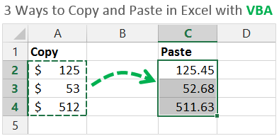
Copy & Paste: The Most Common Excel Action
Copy and paste is probably one of the most common actions you take in Excel. It’s also one of the most common tasks we automate when writing macros.
There are a few different ways to accomplish this task, and the macro recorder doesn’t always give you the most efficient VBA code.
In the following three videos I explain:
- The most efficient method for a simple copy and paste in VBA.
- The easiest way to paste values.
- How to use the PasteSpecial method for other paste types.
You can download the file I use in these videos below. The code is also available at the bottom of the page.
Video #1: The Simple Copy Paste Method
You can watch the playlist that includes all 3 videos at the top of this page.
Video #2: An Easy Way to Paste Values
Video #3: The PasteSpecial Method Explained
VBA Code for the Copy & Paste Methods
Download the workbook that contains the code.
'3 Methods to Copy & Paste with VBA
'Source: https://www.excelcampus.com/vba/copy-paste-cells-vba-macros/
'Author: Jon Acampora

Sub Range_Copy_Examples()
'Use the Range.Copy method for a simple copy/paste

    'The Range.Copy Method - Copy & Paste with 1 line
    Range("A1").Copy Range("C1")
    Range("A1:A3").Copy Range("D1:D3")
    Range("A1:A3").Copy Range("D1")

    'Range.Copy to other worksheets
    Worksheets("Sheet1").Range("A1").Copy Worksheets("Sheet2").Range("A1")

    'Range.Copy to other workbooks
    Workbooks("Book1.xlsx").Worksheets("Sheet1").Range("A1").Copy _
        Workbooks("Book2.xlsx").Worksheets("Sheet1").Range("A1")

End Sub


Sub Paste_Values_Examples()
'Set the cells' values equal to another to paste values

    'Set a cell's value equal to another cell's value
    Range("C1").Value = Range("A1").Value
    Range("D1:D3").Value = Range("A1:A3").Value

    'Set values between worksheets
    Worksheets("Sheet2").Range("A1").Value = Worksheets("Sheet1").Range("A1").Value

    'Set values between workbooks
    Workbooks("Book2.xlsx").Worksheets("Sheet1").Range("A1").Value = _
        Workbooks("Book1.xlsx").Worksheets("Sheet1").Range("A1").Value

End Sub


Sub PasteSpecial_Examples()
'Use the Range.PasteSpecial method for other paste types

    'Copy and PasteSpecial a Range
    Range("A1").Copy
    Range("A3").PasteSpecial Paste:=xlPasteFormats

    'Copy and PasteSpecial a between worksheets
    Worksheets("Sheet1").Range("A2").Copy
    Worksheets("Sheet2").Range("A2").PasteSpecial Paste:=xlPasteFormulas

    'Copy and PasteSpecial between workbooks
    Workbooks("Book1.xlsx").Worksheets("Sheet1").Range("A1").Copy
    Workbooks("Book2.xlsx").Worksheets("Sheet1").Range("A1").PasteSpecial Paste:=xlPasteFormats

    'Disable marching ants around copied range
    Application.CutCopyMode = False

End Sub
Paste Data Below the Last Used Row
One of the most common questions I get about copying and pasting with VBA is, how do I paste to the bottom of a range that is constantly changing? I first want to find the last row of data, then copy & paste below it.
To answer this question, I created a free training video on how to paste data below the last used row in a sheet with VBA. Can I send you the video? Please click the image below to get the video.
Free Training on Macros & VBA
The 3 videos above are from my VBA Pro Course. If you want to learn more about macros and VBA then checkout my free 3-part video training series.
I will also send you info on the VBA Pro Course, that will take you from beginner to expert. Click the link below to get instant access.
Free Training on Macros & VBA
Please leave a comment below with any questions. Thanks!
This article covers everything you need to know about Excel VBA Copy methods.
By “Excel VBA Copy Methods”, I mean the different methods you can use to copy data from one range or worksheet to another.
In this article, I’m going to show you the fastest and most efficient way to copy and filter data no matter what your task is.
I say “Copy and Filter” because in most cases you will want to filter the data before you copy it. If you just want to copy data from one place to another then I cover that too.
The article is broken down as follows:
-
- Which Excel VBA Copy and Filter method is the fastest(section 6) – What the professionals know and how you can use it to your advantage.
- How to pick the best Excel VBA copy method for each task(section 7) – miss this and you’re wasting countless hours of your time.
- How to ensure your application runs at its optimal speed(section
 – It’s not hard to do once you know the secret.
 - The Copy and Filter methods explained with full code examples(sections 9 and 10) – Learn these methods and watch your macros run like magic.
 – It’s not hard to do once you know the secret.
Useful Links
The following are some related articles with more information about certain topics:
Ranges and Cells
Arrays
Dictionary
For Loop
For Each Loop
The Workbook object
The Worksheet object
Glossary
Range.Value2 – returns the underlying value in the call. Value is similar but slower and may not return the correct value if there is currency or data formatting. See this article for more information.
ADO – stands for ActiveX Database Objects. It is a library that allows us to run queries on databases. We can also use it with Excel spreadsheets.
The Webinar
Members of the Webinar Archives can access the webinar for this article by clicking on the image below.
(Note: Website members have access to the full webinar archive.)

Download the Source Code and Data
In this article I will be using the following dataset:

Unless specified, most examples will use the 2 worksheets:
-
-
-
- Transactions – contains the above data.
- Report – the data will be copied to this worksheet.
-
-
How to use this article
In the next section you can see how the different VBA Copy Methods compare in terms of speed. This is vital when you are determining which one to use.
You can use section 4 to help you determine which method you should use based on your requirements.
Section 5 shows you the basic ground work you should have in your application.
The rest of the article provides a description and code example of each method.
Which Excel VBA Copy Method is the Fastest?
In this section you will see how the different methods compare in terms of speed.
Using the fastest method is vital when dealing with large amounts of data. As you can see from the results, some of the methods are incredibly slow.
I have run speed tests on the different methods to see which methods are the fastest for different types of tasks.
I ran the tests on 20000 , 100000 and 200000 records. You can see the average results for each method in milliseconds in the tables below:
Copying Data By Rows

Average time taken by each method in milliseconds
In this test, I filtered by rows that contain a given first name in the first column. About 1% of the records will match the criteria and will be copied. So for 20000 records, there will be 200 records copied.
You can see that using Autofilter and Advanced filter are the fastest methods for copying and filtering rows.
At the other end you can see that a For Loop with Range.Copy takes almost 215 times longer than using AutoFilter. I didn’t even run the 200,000 test for this as I expected it would take 15 minutes plus!
Copying Data By Individual Cells

Average time taken by each method in milliseconds
In this tests we want to copy some of the cells but not the entire row. In most cases we need to copy the cells individually so this makes it more complicated than copying an entire row. This may seem counter intuitive at first that copying serveral cells requires more work than the copying the entire row.
Using the Advanced Filter is the clear winner here. Autofilter doesn’t have it’s own copy method so after filtering we have to copy the data using some other method.
Advanced Filter automatically copies the data and we can specify the columns we want to be copied. Advanced filter then takes care of the rest.
I have created two different methods of copying using AutoFilter for individual rows. The methods may be faster or slower depending on the number of columns:
-
-
-
- The Copy Columns method would be slower with more columns to copy.
- The Delete Columns method would be slower with more columns to delete.
-
-
Copying Data and Summing Totals

Average time taken by each method in milliseconds
In these tests we are summing data for a particular item. Summing means to get the total amount of a given column for a particular item. For example, getting the total volume for “Laptop Model A”.
There are 3 VBA copy methods that we can use to do this. These are:
-
-
-
- Pivot Tables
- For Loop with a Dictionary
- ADO(ActiveX Database Objects)
-
-
Using a Pivot Table is the fastest method for summing data. There is not much difference between the other two methods.
The downside of the Pivot Table is that the code may be slightly complex for a new user. ADO is very flexible but it does require knowledge of SQL(Structured Query Language).
Copying and Transposing Data

Average time taken by each method in milliseconds
Both methods here are pretty fast. If you are doing a large volume of transpose copies then Application.Transpose tends to be quicker than PasteSpecial Transpose.
Which Excel VBA Copy Method Should I Use?
With so many different methods, you may be feeling overwhelmed. Don’t worry, in this section I will provide a complete guide to selecting the correct Excel VBA copy method to use.
Note that you can download the source code for this post from the start or end of this post. This is an invaluable with of practicing the method shown here.
Straight Copy with no Filter
To copy without any filter use the copy by assignment method like this:
shWrite.Range("F1:G4").Value2 = shRead.Range("A1:B4").Value2

Filter columns(AND Logic) and Copy Rows
Advanced Filter is the fastest and easiest method to use if you want to filter by column values using AND logic:
e.g Item is “Laptop Model A” And Volume is greater than 20

Filter columns(OR Logic) and Copy Rows
Advanced Filter is the fastest method to do an OR filter. It’s not possible to do this with AutoFilter.
e.g Item is “Laptop Model A” Or Volume > 20″

Filter and Copy Individual Columns
Sometimes you will not want to copy the entire row. Instead you may want to copy individual columns. Advanced Filter is fastest VBA Copy method for doing this.
e.g. return the columns Item, Volume and Sales where Item is “Laptop Model A” And Volume > 20″

Sum totals for individual items
If you want to get the total amount for each item then using a Pivot Table is faster than the other two methods. ADO(ActiveX Database Objects) is slightly faster than using the For Loop with the Dictionary.

Using a Pivot Table is very flexible. Once you create the table it pretty easy to display the data in many different ways. The downside is that the code may be a bit complex for a VBA beginner.
ADO is much more flexible but requires some knowledge of SQL(a database query language). It also requires using an external library which may be a bit advanced for a VBA beginner.
Using the For Loop and a Dictionary requires more code and is less flexible. But it is still pretty fast for up to 200,000 records and doesn’t require any SQL or external libraries.
Transpose
Transposing means to copy data so that the rows become columns and the columns become rows

There are two methods of transposing data:
- Range.Copy and Transpose using PasteSpecial.
- Assignment and Transpose using Application.Transpose.
There is not much difference between these in terms of speed. However, if your application is doing multiple transpose operations then Range.Copy tends to be much slower.
Before You Start Copying and Filtering
No matter which Excel VBA Copy method we use there are some tasks we must perform first.
These include getting the range of data, turning off certain Excel functionality etc.
We will look at these tasks in this section.
The first thing we will look at is the mistake that most VBA beginners make – using Select.
Never Use Select
When copying data in Excel VBA, don’t use Select – ever!
A big mistake that new VBA users make is thinking that they need to select the cell or range before they copy it.
For example
shRead.Activate
shRead.Range("A1").Select
shWrite.Activate
Selection.Copy ActiveSheet.Range("H1")
Keep these two important things in mind before you use VBA to copy data:
- You don’t need to select the cell or range of cells.
- You don’t need to select or activate the worksheet.
You will see Select used in many places online. But you don’t need to use it for copying cells – ever!
Speed Up Your Code
If you want your code to run fast then it is important to turn off certain VBA functionality at the start of our code. We then turn it back on, at the end of our code.
We can use the following subs to do this:
' Procedure : TurnOffFunctionality
' Source    : www.ExcelMacroMastery.com
' Author    : Paul Kelly
' Purpose   : Turn off automatic calculations, events and screen updating
' https://excelmacromastery.com/
Public Sub TurnOffFunctionality()
    Application.Calculation = xlCalculationManual
    Application.DisplayStatusBar = False
    Application.EnableEvents = False
    Application.ScreenUpdating = False
End Sub

' Procedure : TurnOnFunctionality
' Source    : www.ExcelMacroMastery.com
' Author    : Paul Kelly
' Purpose   : turn on automatic calculations, events and screen updating
' https://excelmacromastery.com/
Public Sub TurnOnFunctionality()
    Application.Calculation = xlCalculationAutomatic
    Application.DisplayStatusBar = True
    Application.EnableEvents = True
    Application.ScreenUpdating = True
End Sub
We can use them like this
Sub Main()

    ' Turn off at the start
    TurnOffFunctionality

    ' Your code here

    ' Turn back on at the end
    TurnOnFunctionality

End Sub
Sometimes when you run your code, it won’t reach the TurnOnFunctionality code.
This could because of an error or because you stop the code at a certain point and don’t restart.
If this happens you can turn everything on again by clicking in the TurnOnFunctionality sub and pressing F5.
Get the correct worksheet
When copying data, we need to specify the range which we will copy from. When using VBA we need to select the worksheet before we can select the range. There are many ways of selecting the worksheet which can be confusing.
I have broken it down into three scenarios:
- The worksheet is in the same workbook as the code.
- The worksheet is in a different workbook but we only want to read from it.
- The worksheet is in a different workbook but we want to write to it.
You can see the code for each of these scenarios in the next subsections:
The worksheet is in the current workbook
The worksheet is in the current workbook so we can use either:
- The code name of the worksheet.
- The worksheet name: ThisWorkbook.Worksheets(“worksheet name”).

In the screenshot below we have changed the codename and worksheet name:

We would use the following code to reference the sheet
' https://excelmacromastery.com/
Sub WorksheetCodeName()

    Dim shRead As Worksheet

    ' Use the code name
    Set shRead = CodeName

    ' OR

    ' Use the worksheet name
    Set shRead = ThisWorkbook.Worksheets("SheetName")

End Sub
The worksheet is in a different workbook – reading only
If the worksheet is in a different workbook than the code, then we need to open the workbook. In this case we will only be reading from the worksheet so we can simply make it read-only.
Then it doesn’t matter if it’s already open. Making it read-only also prevents us from accidentally changing the data in the workbook.
' WorksheetRead()
'
' HOW TO RUN:
' 1. Place this code in a new workbook and save it as a .xlsm file.
' 2. Create a workbook called Writedata.xlsx and place it in the same
'    folder as the workbook you just created.
' 3. Place any value in cell A1 on sheet1 from Writedata.xlsx.
' 4. Run the code(Press F5).
'
' RESULT: The value in cell A1 on sheet1 from Writedata.xlsx
'         will be displayed in a message box.
' https://excelmacromastery.com/
Sub WorksheetRead()

    ' Get the full filename and path of "WriteData.xlsx"
    Dim sFilename As String
    sFilename = _
         ThisWorkbook.Path & Application.PathSeparator & "WriteData.xlsx"

    ' Open workbook as read-only and store in variable wk
    Dim wk As Workbook
    Set wk = Workbooks.Open(sFilename, ReadOnly:=True)

    ' Store the worksheet Sheet1 in the variable shRead
    Dim shRead As Worksheet
    Set shRead = wk.Worksheets("Sheet1")

    ' Print the value from the worksheet cell A1
    If IsEmpty(shRead.Range("A1").Value2) Then
        MsgBox "No value was found in cell Sheet1:A1 of WriteData.xlsx."
    Else
        MsgBox "The value found in Sheet1:A1 is of WriteData.xlsx is: " _
            & shRead.Range("A1").Value2
    End If

    wk.Close SaveChanges:=False
End Sub
The worksheet is in a different workbook – reading and writing
Just like the last example, the worksheet is in a different workbook than the code. In this case we want to write to the worksheet in the workbook.
We first check if the workbook is already open, and if so we display a message informing the user to close it before running the code again:
' WorksheetWrite()
'
' HOW TO RUN:
' 1. Place this code in a new workbook and save it as a .xlsm file.
' 2. Create a workbook called Writedata.xlsx and place it in the same
'    folder as the workbook you just created.
' 3. Click in the WorksheetWrite sub and press F5 to run the code.
' 4. Open the Writedata.xlsx and check if the value was correctly
'    written to cell A1 in sheet1.
'
' RESULT: If the file is already open then and error message will be
'         displayed to the user asking them to close the file.
'         If the file is not already open then the value 99 will be
'         written to cell A1 on sheet1 of Writedata.xlsx.
' https://excelmacromastery.com/
Sub WorksheetWrite()

    Dim sFilename As String
    sFilename = _
         ThisWorkbook.Path & Application.PathSeparator & "WriteData.xlsx"

    ' Ensure that the workbook is not already open
    If IsWorkBookOpen("WriteData.xlsx") Then
        MsgBox "Please close workbook " & sFilename & " and try again."
        Exit Sub
    End If

    ' Open workbook and store in variable wk
    Dim wk As Workbook
    Set wk = Workbooks.Open(sFilename, ReadOnly:=False)

    ' Store the worksheet Sheet1 in the variable shRead
    Dim shRead As Worksheet
    Set shRead = wk.Worksheets("Sheet1")

    ' Write a value to the worksheet cell A1
    shRead.Range("A1").Value2 = Now

    ' Close the file when finished with it
    wk.Close saveChanges:=True

End Sub

' Helper function to check if workbook is already open
Function IsWorkBookOpen(strBookName As String) As Boolean

    Dim oBk As Workbook

    On Error Resume Next
    Set oBk = Workbooks(strBookName)
    On Error GoTo 0

    If Not oBk Is Nothing Then
        IsWorkBookOpen = True
    End If

End Function
Now that we can get any worksheet we require, we can focus on how to copy the data.
Get the Data Range
In many online Excel VBA Copy examples, you will see a fixed range like Range(“A1:D6”).
When dealing with real-world applications it is rare that the data will be of a fixed size.
For example, imagine you stored student marks for each class in a worksheet. Obviously, each class will have a different number of students. Each time you read a worksheet you cannot be sure in advance what the range will be.
Your code should be able to figure out the full range of data, even if the size changes each time it runs.
There are two types of data:
- Rectangular data where the data is in a list of rows with no blank rows or columns.
- Fragmented data where the data may contain blank rows or columns.
Using CurrentRegion
The CurrentRegion property of Range is very useful for returning the entire range of data. CurrentRegion returns all the adjacent data from a given range.
You can see the CurrentRegion in Excel by selecting a cell and pressing Ctrl + Shift + *.
In the screenshot below you can see two groups of adjacent data. By selecting any cell with data and pressing Ctrl + Shift + *, Excel will select all the data in that group. This is the current region.

We can also use the CurrentRegion in VBA:
The Current region will work as long as there are no blank rows or columns between the data.
' CurrentRegion()
'
' HOW TO RUN:
' 1. Create a worksheet called "CurrentRegion".
' 2. Add data to all cells in the range B3:D14.
' 3. Run this sub(F5).
'
' RESULT: The current region for B3, C9 and D14 will
'         be displayed in the Immediate Window(Ctrl + G).
' https://excelmacromastery.com/
Sub CurrentRegion()

     ' Get the worksheets
    Dim shRead As Worksheet
    Set shRead = ThisWorkbook.Worksheets("CurrentRegion")

    Dim rg1 As Range, rg2 As Range, rg3 As Range

    ' Get the current region
    ' All the below examples with return B3:D14
    Set rg1 = shRead.Range("B3").CurrentRegion
    Set rg2 = shRead.Range("C9").CurrentRegion
    Set rg3 = shRead.Range("D14").CurrentRegion

    ' Display the addresses to the Immediate Window(Ctrl + G)
    Debug.Print "B3 CurrentRegion is: " & rg1.Address
    Debug.Print "C9 CurrentRegion is: " & rg2.Address
    Debug.Print "D14 CurrentRegion is: " & rg3.Address

End Sub
Using End with xlUp and xlToLeft
If there are blank rows and/or blank columns then CurrentRegion will not return all the data.
For example, in the data shown here there are blank rows and a blank column:

We need to get the last row with data and/or the last column with data. We can then use these cells to build our Range.
' UseLastRowCol()
'
' HOW TO RUN:
' 1. Create a worksheet called "Fragmented".
' 2. Add any data to the cells A1:E13 but make sure you
'    have the same blank cells as in the above screenshot.
' 3. Run this sub(F5)
'
' RESULT: The range A1:E13 will be displayed in the
'         Immediate Window(Ctrl + G).
' https://excelmacromastery.com/
Sub UseLastRowCol()

     ' Get the worksheet
    Dim shRead As Worksheet
    Set shRead = ThisWorkbook.Worksheets("Fragmented")

    Dim lastRow As Long, lastCol As Long

    ' Get the last cell with data in column A
    lastRow = shRead.Cells(shRead.Rows.count, 1).End(xlUp).row

    ' Get the last cell with data in row 1
    lastCol = shRead.Cells(1, shRead.Columns.count).End(xlToLeft).column

    Dim rg As Range
    With shRead
        ' Get the full range of data from A1 to last row and column
        Set rg = .Range(.Cells(1, 1), .Cells(lastRow, lastCol))
    End With

    ' Print the rg address(i.e. A1:E13) to the Immediate Window(Ctrl + G)
    Debug.Print "The range of data is: " & rg.Address

End Sub
Excel VBA Copy Methods
In this section we are going to look at the copying methods.
There are three ways of copying data in VBA:
- The Range.Copy function
- The assignment operator(i.e. equals sign)
- The Range.CopyFromRecordset function(ADO only)
In the following sub sections we will look at these in turn. We will be using these Excel VBA copy methods with the different filter methods.
Range.Copy
We can use the Copy method of the Range to copy data.
' https://excelmacromastery.com/
Sub SimpleCopy()

     ' Get the worksheet
    Dim shRead As Worksheet
    Set shRead = ThisWorkbook.Worksheets("Transactions")

    ' Copy the data from A1:D1 to H1:K1
    shRead.Range("A1:D1").Copy Destination:=shRead.Range("H1")

    ' Using Destination is optional
    shRead.Range("A1:D1").Copy shRead.Range("H1")

End Sub
We can copy between worksheets using this Excel VBA method. The only thing that will change in the code is the worksheets that we use.
' UsingRangeCopy()
'
' HOW TO RUN:
' 1. Create a workbook called Data.xlsx and place it in the same
'    folder as the workbook with the code.
' 2. Rename sheet1 to "CustomerData".
' 3. Add data to the range A1:D19.
' 4. Save the file.
' 5. Have a worksheet called "Report" in the current workbook
' 6. Click in this sub and press F5 to run
'
' RESULT: The data in the range A1:D19 from the CustomerData
'          worksheet in Data.xlsx will have been copied to
'         the Report worksheet in the current workbook.
' https://excelmacromastery.com/
Sub UsingRangeCopy()

    Dim sFilename As String
    sFilename = _
            ThisWorkbook.Path & Application.PathSeparator & "Data.xlsx"

    ' Open a workbook called Data.xlsx from the current folder
    Dim wk As Workbook
    Set wk = Workbooks.Open(sFilename, ReadOnly:=True)

    ' shRead stores the worksheet CustomerData
    ' shWrite store the Report sheet
    Dim shRead As Worksheet, shWrite As Worksheet
    Set shRead = wk.Worksheets("CustomerData")
    Set shWrite = ThisWorkbook.Worksheets("Report")

    ' Clear the data from the report worksheet
    shWrite.Cells.Clear

    ' Copy from CustomerData to Report
    shRead.Range("A1:D19").Copy shWrite.Range("A1")

    ' Activate the report worksheet
    shWrite.Activate

    ' Close the "Data.xlsx" workbook
    wk.Close

End Sub
This Range.Copy method copies everything. In other words it will copy values, formulas, formats etc.
If we only want to copy the data we can use the PasteSpecial property of Range.
Using PasteSpecial
We can use PasteSpecial with Range.Copy to paste the values only
' https://excelmacromastery.com/
Sub UsingPasteSpecial()

    ' Get the worksheets
    Dim shRead As Worksheet, shWrite As Worksheet
    Set shRead = ThisWorkbook.Worksheets("Transactions")
    Set shWrite = ThisWorkbook.Worksheets("Report")

    ' Clear any existing data from report
    shWrite.Cells.Clear

    ' This will copy the values only
    shRead.Range("A1:E13").Copy
    shWrite.Range("A1").PasteSpecial xlPasteValues

End Sub
You can also copy formats, formulas and comments using PasteSpecial. You can read more about it here.
Range.Copy and Transpose
Transposing data means that the rows become columns and the columns become rows:
We can use the Range.PasteSpecial function to transpose data:
' https://excelmacromastery.com/
Sub RangeCopy_Transpose()

    ' Get the worksheets
    Dim shRead As Worksheet
    Set shRead = ThisWorkbook.Worksheets("Transpose")

    ' Clear any existing data
    shRead.Range("F1:I2").Clear

    ' This will copy from A1:B4 to F1:I2
    shRead.Range("A1:B4").Copy
    shRead.Range("F1").PasteSpecial Transpose:=True

End Sub
Copying by Assignment
We can assign values using the equals sign in VBA.
We can copy values from one range to another using assignment.
The value to the right of the equals is placed in cell to the left of the equals as you can see in these examples:
' https://excelmacromastery.com/
Sub AssignExamples()"

    ' Copy a value to a cell
    Range("A1").Value2 = 56
    Range("A2").Value2 = "Mary"

    ' Copy cell to cell
    Range("G1").Value2 = Range("F1").Value2
    Range("G2").Value2 = Range("F2").Value2

    ' Copy multiple cells - the source and destination range
    ' must be the same size
    Range("A1:C5").Value2 = Range("D1:F5").Value2

End Sub
The code below shows an example of copying the data from the data shown in the screenshot at the start of this section.
We will copy the range A1:D11 on the worksheet Transactions to the range A1:D11 on worksheet Report.
' UsingAssignment()
'
' Requirements:
' 1. A worksheet "Transactions" containing data from this
' section: "The Dataset for this Article".
' 2. A worksheet for output called "Report".
'
' RESULT: The data will be copied from the Transaction worksheet
'         to the report worksheet
' https://excelmacromastery.com/
Sub UsingAssignment()

    ' Get the worksheets
    Dim shRead As Worksheet, shWrite As Worksheet
    Set shRead = ThisWorkbook.Worksheets("Transactions")
    Set shWrite = ThisWorkbook.Worksheets("Report")

    With shWrite

        ' Clear the data in output worksheet
        .Cells.ClearContents

        ' Set the cell formats
        .Columns(2).NumberFormat = "dd/mm/yyyy"
        .Columns(3).NumberFormat = "$#,##0;[Red]$#,##0"
        .Columns(4).NumberFormat = "0"
        .Columns(5).NumberFormat = "$#,##0;[Red]$#,##0"

    End With

    ' Copy the data
    shWrite.Range("A1:D11").Value2 = shRead.Range("A1:D11").Value2

End Sub
The key thing to remember about assigning values is that the destination must be the same size as the source.
If it is smaller than the source range then not all the data will be written.
If it is bigger than the source then there will be #N/A errors in the extra cells.
Assignment with Transpose
We can use the WorksheetFunction.Transpose function to transpose using the assignment operator(i.e. equals sign) to copy:
' https://excelmacromastery.com/
Sub TransposeAssign()

    ' Get the worksheets
    Dim shRead As Worksheet
    Set shRead = ThisWorkbook.Worksheets("Transpose")

    ' Clear any existing data
    shRead.Range("F1:I2").Clear

    shRead.Range("F1:I2").Value2 = _
            WorksheetFunction.Transpose(shRead.Range("A1:B4").Value2)

End Sub
Using Range.CopyFromRecordset
A Recordset is the collection of data we get when we run a database query.
We can run database queries on worksheet data using ADO (ActiveX Data Objects).
We will look at this Excel VBA Copy method in more detail in the ADO section below.
Excel VBA Filter Methods
Whenever you are copying data in VBA you will almost always apply some type of filter. This could be selection rows based on certain criteria or it could be summing data.
In this section, we are going to look at the various ways of filtering data. If you want working examples using the Filter methods then you can download the source code at the top or bottom of this post.
Filtering using For and If
The most common way of filtering data in VBA is using a For Loop and If Statement.
This is the least flexible and most long-winded method of filtering data in VBA. By long-winded, I mean that it requires lots of code compared to the other methods.
Using For and IF is the method you will see used the most in examples or in legacy VBA code.
We use the For Loop to read through data one row at a time. For each row, we will use the If Statement to check for certain criteria.
Here is a simple outline:
' https://excelmacromastery.com/
Sub ForIf_Basic()

    ' Get the worksheets
    Dim shRead As Worksheet
    Set shRead = ThisWorkbook.Worksheets("Transactions")

    Dim i As Long
    For i = 1 To 13
        If shRead.Range("A" & i).Value2 = "Laptop Model A" Then
            ' Code for copying here
        End If
    Next i

End Sub
We can use both And and Or operators in the if statement.
Here are some examples:
If Item = "Laptop Model A" And Volume > 20 Then

If Item = "Laptop Model A" Or Volume > 20 Then

If Item = "Laptop Model A" Or Item = "Laptop Model B" Then
How to Copy Rows
The following code reads through the data. It checks each line to see if the first cell contains “Laptop Model A” .
If the row with these criteria is found, the row will be copied to the output worksheet.
The first version of the code below will use Range.Copy and the second will use the assign copy method:
' For_RangeCopy()
'
' Requirements:
' 1. A worksheet "Transactions" containing data from this
' section: "The Dataset for this Article".
' 2. A worksheet for output called "Report".
'
' https://excelmacromastery.com/
Sub For_RangeCopy()

    ' Get the worksheets
    Dim shRead As Worksheet
    Set shRead = ThisWorkbook.Worksheets("Transactions")

    Dim shWrite As Worksheet
    Set shWrite = ThisWorkbook.Worksheets("Report")

    ' Get the range
    Dim rg As Range
    Set rg = shRead.Range("A1").CurrentRegion

    With shWrite

        ' Clear the data in output worksheet
        .Cells.ClearContents

        ' Set the cell formats
        .Columns(2).NumberFormat = "dd/mm/yyyy"
        .Columns(3).NumberFormat = "$#,##0;[Red]$#,##0"
        .Columns(4).NumberFormat = "0"
        .Columns(5).NumberFormat = "$#,##0;[Red]$#,##0"

    End With

    ' Read through the data
    Dim i As Long, row As Long
    row = 1
    For i = 1 To rg.Rows.count

        If rg.Cells(i, 1).Value2 = "Laptop Model A" Or i = 1 Then

            ' Copy using Range.Copy
            rg.Rows(i).Copy
            shWrite.Range("A" & row).PasteSpecial xlPasteValues

            ' move to the next output row
            row = row + 1

        End If

    Next i

End Sub
' For_Assign()
'
' Requirements:
' Requirements:
' 1. A worksheet "Transactions" containing data from this
' section: "The Dataset for this Article".
' 2. A worksheet for output called "Report".
'
' https://excelmacromastery.com/
Sub For_Assign()

    ' Get the worksheets
    Dim shRead As Worksheet
    Set shRead = ThisWorkbook.Worksheets("Transactions")

    Dim shWrite As Worksheet
    Set shWrite = ThisWorkbook.Worksheets("Report")

    ' Get the range
    Dim rg As Range
    Set rg = shRead.Range("A1").CurrentRegion
    With shWrite

        ' Clear the data in output worksheet
        .Cells.ClearContents

        ' Set the cell formats
        .Columns(2).NumberFormat = "dd/mm/yyyy"
        .Columns(3).NumberFormat = "$#,##0;[Red]$#,##0"
        .Columns(4).NumberFormat = "0"
        .Columns(5).NumberFormat = "$#,##0;[Red]$#,##0"

    End With

    ' Read through the data
    Dim i As Long, row As Long
    row = 1
    For i = 1 To rg.Rows.count

        If rg.Cells(i, 1).Value2 = "Laptop Model A" Or i = 1 Then

            ' Get the destination range
            Dim rgDest As Range
            Set rgDest = _
                shWrite.Range("A" & row).Resize(1, rg.Columns.count)

            ' Copy using Assignment
            rgDest.Value2 = rg.Rows(i).Value2

            ' move to the next output row
            row = row + 1

        End If

    Next i

End Sub
In the above code, we use Range.Resize when copying by assignment. You can read more about this here.
Using an Array to Read Faster
If you are reading through a lot of data then reading directly from the worksheet range is very slow.
It is much quicker to copy the data to an array and then read through that array. Then when we are finished, we write the array back to the worksheet
We cannot use Range.Copy because it obviously can only be used on an actual range.
Let’s update our last example so it will use an array:
' https://excelmacromastery.com/
Sub ForUsingArray_Assign()

    ' Get the worksheets
    Dim shRead As Worksheet
    Set shRead = ThisWorkbook.Worksheets("Transactions")

    Dim shWrite As Worksheet
    Set shWrite = ThisWorkbook.Worksheets("Report")

    ' Copy the range to an array
    Dim arr As Variant
    arr = shRead.Range("A1").CurrentRegion.Value2

    With shWrite
        ' Clear the data in output worksheet
        .Cells.ClearContents

        ' Set the cell formats
        .Columns(2).NumberFormat = "dd/mm/yyyy"
        .Columns(3).NumberFormat = "$#,##0;[Red]$#,##0"
        .Columns(4).NumberFormat = "0"
        .Columns(5).NumberFormat = "$#,##0;[Red]$#,##0"

    End With

    ' Read through the data
    Dim i As Long, j As Long
    Dim row As Long, Columns As Long
    row = 1
    For i = LBound(arr) To UBound(arr)

        ' If "Laptop Model A" or header row then copy
        If arr(i, 1) = "Laptop Model A" Or i = 1 Then

            ' Copy each column
            For j = LBound(arr, 2) To UBound(arr, 2)
                shWrite.Cells(row, j).Value2 = arr(i, j)
            Next j

            ' move to the next output row
            row = row + 1

        End If

    Next i

End Sub
We could also use the Worksheet Function Index to copy. However, it is incredibly slow. In the speed tests it was over 4000 times slower than using the AutoFilter.
' Copy using Index
Columns = UBound(arr, 2)
shRepAssign.Range("A" & row).Resize(1, Columns).Value2 = _
        Application.WorksheetFunction.Index(arr, i, 0)
Copying Individual Fields
Copying individual items in a row is actually very straightforward.
We simply copy each cell individually:
' For_Assign_Individual()
'
' Requirements:
' 1. A worksheet "Transactions" containing data from this
' section: "The Dataset for this Article".
' 2. A worksheet for output called "Report".
'
' https://excelmacromastery.com
Sub For_Assign_Individual()

    ' Get the worksheets
    Dim shRead As Worksheet
    Set shRead = ThisWorkbook.Worksheets("Transactions")

    Dim shWrite As Worksheet
    Set shWrite = ThisWorkbook.Worksheets("Report")

    ' Get the range
    Dim rg As Range
    Set rg = shRead.Range("A1").CurrentRegion

    With shWrite
        ' Clear the data in output worksheet
        .Cells.ClearContents

        ' Set the cell formats
        .Columns(2).NumberFormat = "$#,##0;[Red]$#,##0"

    End With

    ' Read through the data
    Dim i As Long, rgWrite As Range, row As Long
    row = 1
    For i = 1 To rg.Rows.count

        ' If "Laptop Model A" or the header row
        If rg.Cells(i, 1).Value2 = "Laptop Model A" Or i = 1 Then

            ' Copy from column A to column A
            shWrite.Cells(row, 1).Value2 = rg.Cells(i, 1).Value2

            ' Copy from column E to column B
            shWrite.Cells(row, 2).Value2 = rg.Cells(i, 5).Value2

            ' Move to the next row for writing
            row = row + 1

        End If

    Next i

End Sub
The method below using Range.Copy – it is very slow so it is best to avoid using it.
' WARNING: DON'T USED THIS METHOD - IT IS INCREDIBLY SLOW
' https://excelmacromastery.com/
Sub For_RangeCopy_Individual()

    ' Get the worksheets
    Dim shRead As Worksheet
    Set shRead = ThisWorkbook.Worksheets("Transactions")

    Dim shWrite As Worksheet
    Set shWrite = ThisWorkbook.Worksheets("Report")

    With shWrite

        ' Clear the data in output worksheet
        .Cells.ClearContents

        ' Set the cell formats
        .Columns(2).NumberFormat = "$#,##0;[Red]$#,##0"

    End With

    ' Get the range
    Dim rg As Range
    Set rg = shRead.Range("A1").CurrentRegion

    ' Read through the data
    Dim i As Long, rgWrite As Range, row As Long
    row = 1
    For i = 1 To rg.Rows.count

        ' If "Laptop Model A" or the header row
        If rg.Cells(i, 1).Value2 = "Laptop Model A" Or i = 1 Then

            ' Copy using Range.Copy
            rg.Cells(i, 1).Copy
            shWrite.Range("A" & row).PasteSpecial xlPasteValues

            rg.Cells(i, 5).Copy
            shWrite.Range("B" & row).PasteSpecial xlPasteValues

            ' Move to the next row for writing
            row = row + 1

        End If

    Next i
In this example we use an array with the For loop to copy. It is the fastest way to copy individual columns using the For loop but it is still way slower than using the AutoFilter.
' ForUsingArray_Assign_Individual()
'
' Requirements:
' 1. A worksheet "Transactions" containing data from this
' section: "The Dataset for this Article".
' 2. A worksheet for output called "Report".
'
' https://excelmacromastery.com/
Sub ForUsingArray_Assign_Individual()

    ' Get the worksheets
    Dim shRead As Worksheet
    Set shRead = ThisWorkbook.Worksheets("Transactions")

    Dim shWrite As Worksheet
    Set shWrite = ThisWorkbook.Worksheets("Report")

    With shWrite

        ' Clear the data in output worksheet
        .Cells.ClearContents

        ' Set the cell formats
        .Columns(2).NumberFormat = "$#,##0;[Red]$#,##0"

    End With

    ' Get the range
    Dim arr As Variant
    arr = shRead.Range("A1").CurrentRegion.Value2

    ' Read through the data
    Dim i As Long, rgWrite As Range, row As Long
    row = 1
    For i = LBound(arr) To UBound(arr)

        ' If "Laptop Model A" or the header row
        If arr(i, 1) = "Laptop Model A" Or i = 1 Then

            ' Copy from column A to column A on the report worksheet
            shWrite.Cells(row, 1).Value2 = arr(i, 1)

            ' Copy from column E to column B on the report worksheet
            shWrite.Cells(row, 2).Value2 = arr(i, 5)

            ' Move to the next row for writing
            row = row + 1

        End If

    Next i

End Sub
If the original data has a lot of columns and you only require a few of them, then this method may be as fast as AutoFilter but you will need to test both methods.
Summing Totals
In the data shown below we want to get the total sales for each item:

Our result should look like this:
Summing data like this is much trickier than simply filtering data.
For each item, we need to store a running total somewhere. Each time we read an item we need to either create a new entry or add the current sales amount to the existing entry.
The easiest way to do this is to use a Dictionary.
You can see the code to do this below. You will notice that it is split into two parts:
- In part one we read the values from the worksheet to the dictionary.
- In part two we write the values from the dictionary to the worksheet.
' ForDictionary_Assign_Sum()
'
' Requirements:
' 1. A worksheet "Transactions" containing data from this
' section: "The Dataset for this Article".
' 2. A worksheet for output called "Report".
'
' IMPORTANT: Add the Dictionary reference to use the dictionary
'            Tools->Reference and check "Microsoft Scripting Runtime"
' https://excelmacromastery.com/
Sub ForDictionary_Assign_Sum()

    ' PART 1 - Read the data
    ' Get the worksheets
    Dim shRead As Worksheet
    Set shRead = ThisWorkbook.Worksheets("Transactions")

    ' Get the range
    Dim rg As Range
    Set rg = shRead.Range("A1").CurrentRegion

    ' Create the dictionary
    Dim dict As New Dictionary

    ' Read through the data
    Dim i As Long, Item As String, Sales As Long
    For i = 2 To rg.Rows.count
        ' Store the values in a variable
        Item = rg.Cells(i, 1).Value2
        Sales = rg.Cells(i, 5).Value2

        ' The item will be automatically added if it doesn't exist
        dict(Item) = dict(Item) + Sales
    Next i

    ' PART 2 - Write the data
    Dim shWrite As Worksheet
    Set shWrite = ThisWorkbook.Worksheets("Report")

    With shWrite

        ' Clear the data in output worksheet
        .Cells.ClearContents

        ' Set the cell formats
        .Columns(2).NumberFormat = "$#,##0;[Red]$#,##0"

        ' Write header
        .Cells(1, 1).Value2 = "Item"
        .Cells(1, 2).Value2 = "Sales"

    End With

    Dim key As Variant, row As Long
    row = 2
    ' Read through each item in the Dictionary
    For Each key In dict.Keys

        shWrite.Cells(row, 1) = key
        shWrite.Cells(row, 2) = dict(key)

        row = row + 1
    Next key

End Sub
Summing Multiple Totals
In the previous example we were summing one item. This time we are going to sum the volume and the price fields.
The Dictionary stores a key and a value. If we want to store more than one value then we use a class module.
In the next example, I have split up the code into procedures to make it easier to read and to be more flexible:
' Class Module: clsSales
Public Items As String
Public Volume As Long
Public Sales As Long
' https://excelmacromastery.com/
Sub CreateReport()

    ' Declare a Dictionary variable
    Dim dict As Dictionary

    ' Read the data to the Dictionary
    Set dict = ReadData

    ' Write the Data from the Dictionary to the Worksheet
    WriteData dict

End Sub

' Read the data from the worksheet into a Dictionary
'
' IMPORTANT: Add the Dictionary reference to use the dictionary
' Tools->Reference and check "Microsoft Scripting Runtime"
' https://excelmacromastery.com/
Private Function ReadData() As Dictionary

    ' Create the dictionary
    Dim dict As New Dictionary

    ' Get the worksheets
    Dim shRead As Worksheet
    Set shRead = ThisWorkbook.Worksheets("Transactions")

    ' Get the range
    Dim rg As Range
    Set rg = shRead.Range("A1").CurrentRegion

    ' Read through the data
    Dim i As Long, Item As String, Volume As Long, Sales As Long
    Dim oSales As clsSales, oSalesCurrent As clsSales
    For i = 2 To rg.Rows.count

        Item = rg.Cells(i, 1).Value2
        Volume = rg.Cells(i, 4).Value2
        Sales = rg.Cells(i, 5).Value2

        ' Check if the Item has already been added
        If dict.Exists(Item) = False Then
            ' Add Item and new class module object
            Set oSales = New clsSales
            dict.Add Item, oSales
        End If

        ' Get the current item
        Set oSalesCurrent = dict(Item)

        ' Update the data
        With oSalesCurrent
            .Volume = .Volume + Volume
            .Sales = .Sales + Sales
        End With

    Next i

    Set ReadData = dict

End Function

' Write the summed data to the worksheet
' https://excelmacromastery.com/
Sub WriteData(dict As Dictionary)

    Dim shWrite As Worksheet
    Set shWrite = ThisWorkbook.Worksheets("Report")

    With shWrite

        ' Clear the data in output worksheet
        .Cells.ClearContents

        ' Set the cell formats
        .Columns(2).NumberFormat = "0"
        .Columns(3).NumberFormat = "$#,##0;[Red]$#,##0"

        ' Write header
        .Cells(1, 1).Value2 = "Item"
        .Cells(1, 2).Value2 = "Volume"
        .Cells(1, 3).Value2 = "Sales"

    End With

    Dim key As Variant, oData As clsSales, row As Long
    row = 2

    ' Read through each item in the Dictionary
    For Each key In dict.Keys

        Set oData = dict(key)

        shWrite.Cells(row, 1) = key
        shWrite.Cells(row, 2) = oData.Volume
        shWrite.Cells(row, 3) = oData.Sales

        row = row + 1

    Next key

End Sub
Using AutoFilter
The methods that we have looked at so far require a lot of code.
There is actually a much simpler way of reading and filtering data. We can use the AutoFilter. This is the filter we use in Excel to filter data. Once the data is filtered we can easily copy and paste it.

VBA AutoFilter Excel
In terms of speed, AutoFilter came out on top in the speed tests that I performed. It is the best one to use for selecting or copying either rows or individual columns.
These are some examples of using AutoFilter in VBA:
' Field 1 = "Ipsum Corporation" and field 3 >=50
rg.AutoFilter Field:=1, Criteria1:="Ipsum Corporation" _
       , Operator:=xlAnd, Field:=3, Criteria1:=">=50"

' Field 1 starts with "I"
rg.AutoFilter Field:=1, Criteria1:="I*"

' Field 1 ends with "Ltd"
rg.AutoFilter Field:=1, Criteria1:="*Ltd"

' Field 1 contains "Su"
rg.AutoFilter Field:=1, Criteria1:="*Su*"

' Field 1 does not contain "Su"
rg.AutoFilter Field:=1, Criteria1:="<>*Su*"

' Get the top 10 items based on the value in Field 3
rg.AutoFilter Field:=3, Criteria1:="10", Operator:=xlTop10Items

' Field 3 is in the value list of 100,17 and 2
rg.AutoFilter Field:=3, Criteria1:=Array("100", "17", "2") _
     , Operator:=xlFilterValues
Now that we understand the basics, let’s look at some practical examples of using AutoFilter.
How to Copy Rows
Using AutoFilter is the fastest way to copy filtered rows of data.
Let’s use AutoFilter to copy all the rows that contain “Laptop Model A”.
The following code shows how to do this:
' AutoFilter_RangeCopy_Row()
'
' Requirements:
' 1. A worksheet "Transactions" containing data from this
' section: "The Dataset for this Article".
' 2. A worksheet for output called "Report".
'
' https://excelmacromastery.com/
Sub AutoFilter_RangeCopy_Row()

    ' Get the worksheets
    Dim shRead As Worksheet, shWrite As Worksheet
    Set shRead = ThisWorkbook.Worksheets("Transactions")
    Set shWrite = ThisWorkbook.Worksheets("Report")

    With shWrite
        ' Clear the data in output worksheet
        .Cells.ClearContents

        ' Set the cell formats
        .Columns(2).NumberFormat = "dd/mm/yyyy"
        .Columns(3).NumberFormat = "$#,##0;[Red]$#,##0"
        .Columns(4).NumberFormat = "0"
        .Columns(5).NumberFormat = "$#,##0;[Red]$#,##0"

    End With

    ' Get the range
    Dim rg As Range
    Set rg = shRead.Range("A1").CurrentRegion

    ' Remove any existing filters
    rg.AutoFilter

    ' Apply the Autofilter
    rg.AutoFilter Field:=1, Criteria1:="Laptop Model A"

    ' Copy the data using Range Copy
    shRead.Range("A1").CurrentRegion.SpecialCells(xlCellTypeVisible).Copy
    shWrite.Range("A1").PasteSpecial xlPasteValues

    ' Remove any existing filters
    rg.AutoFilter

    ' Active the output sheet so it is visible
    shWrite.Activate

End Sub
We can also use assign to copy the data. It is almost as fast but requires slightly more complex code.
It is actually not necessary to use this code but I am including it for completeness:
' AutoFilter_Assign_Row()
'
' Requirements:
' 1. A worksheet "Transactions" containing data from this
' section: "The Dataset for this Article".
' 2. A worksheet for output called "Report".
'
' https://excelmacromastery.com/
Sub AutoFilter_Assign_Row()

    ' Get the worksheets
    Dim shRead As Worksheet, shWrite As Worksheet
    Set shRead = ThisWorkbook.Worksheets("Transactions")
    Set shWrite = ThisWorkbook.Worksheets("Report")

    With shWrite

        ' Clear the data in output worksheet
        .Cells.ClearContents

        ' Set the cell formats
        .Columns(2).NumberFormat = "dd/mm/yyyy"
        .Columns(3).NumberFormat = "$#,##0;[Red]$#,##0"
        .Columns(4).NumberFormat = "0"
        .Columns(5).NumberFormat = "$#,##0;[Red]$#,##0"

    End With

    ' Get the range
    Dim rg As Range
    Set rg = shRead.Range("A1").CurrentRegion

    ' Remove any existing filters
    rg.AutoFilter

    ' Apply the Autofilter
    rg.AutoFilter Field:=1, Criteria1:="Laptop Model A"

    ' Get the read range
    Dim rgRead As Range
    Set rgRead = _
        shRead.Range("A1").CurrentRegion.SpecialCells(xlCellTypeVisible)

    Dim rgRow As Range, row As Long
    row = 1
    ' Read through each row
    For Each rgRow In rgRead.Rows

        ' Copy the row
        shWrite.Cells(row, 1).Resize(1, rgRead.Columns.count).Value2 _
                   = rgRow.Value2

        ' move to the next output row
        row = row + 1

    Next rgRow

    ' Remove any existing filters
    rg.AutoFilter

End Sub
Using AutoFilter code is much easier to write because we don’t need a For Loop and an If Statement. We can filter the data in just one line.
Copying Individual Fields
Copy individual cells is more long winded than copying the row.
It may seem counter intuitive at first but we have to specify the cells we are copying. With a row, we can just copy the entire thing.
There are 2 main ways we can do this:
- Copy the individual columns from the filtered data.
- Copy filtered data and delete the columns that are not required.
Copy the Columns
The first method is the most basic way to do this. We simple copy each column that we require
' AutoFilter_CopyColumns()
'
' Requirements:
' 1. A worksheet "Transactions" containing data from this
' section: "The Dataset for this Article".
' 2. A worksheet for output called "Report".
'
' Details: Use AutoFilter with Range.Copy to filter and copy individual
'          column data.
'          The resulting data should contain the columns Items and Sales.
' https://excelmacromastery.com/
Sub AutoFilter_CopyColumns()

    ' Get the worksheets
    Dim shRead As Worksheet, shWrite As Worksheet
    Set shRead = ThisWorkbook.Worksheets("Transactions")
    Set shWrite = ThisWorkbook.Worksheets("Report")

    With shWrite

        ' Clear the data in output worksheet
        .Cells.ClearContents

        ' Set the cell formats
        .Columns(2).NumberFormat = "$#,##0;[Red]$#,##0"

    End With

    ' Get the range
    Dim rg As Range
    Set rg = shRead.Range("A1").CurrentRegion

    ' Remove any existing filters
    rg.AutoFilter

    ' Apply the Autofilter
    rg.AutoFilter Field:=1, Criteria1:="Laptop Model A"

    Dim arr As Variant
    arr = Array(1, 5)

    ' Remove unnecessary columns
    Dim i As Long, column As Long
    column = 1
    For i = LBound(arr) To UBound(arr)
        rg.Cells(1, arr(i)).EntireColumn.Copy
        shWrite.Cells(1, column).PasteSpecial xlPasteValues
        column = column + 1
    Next i

    ' Remove any existing filters
    rg.AutoFilter

End Sub
Copy and Delete Unwanted Columns
The second method is the fastest for data with a reasonable number of columns. We simply copy all the data and delete the columns we don’t need:
' AutoFilter_DeleteColumns()
'
' Requirements:
' 1. A worksheet "Transactions" containing data from this
' section: "The Dataset for this Article".
' 2. A worksheet for output called "Report".
'
' Details: Use AutoFilter with Range.Copy to filter and copy individual
'          column data.
'          Copy the entire data and then delete the unnecessary columns.
'          The result should be Item and Sales columns only.
' https://excelmacromastery.com/
Sub AutoFilter_DeleteColumns()

    ' Get the worksheets
    Dim shRead As Worksheet, shWrite As Worksheet
    Set shRead = ThisWorkbook.Worksheets("Transactions")
    Set shWrite = ThisWorkbook.Worksheets("Report")

    With shWrite

        ' Clear the data in output worksheet
        .Cells.ClearContents

        ' Set the cell formats
        .Columns(2).NumberFormat = "$#,##0;[Red]$#,##0"

    End With

    ' Get the range
    Dim rg As Range
    Set rg = shRead.Range("A1").CurrentRegion

    ' Remove any existing filters
    rg.AutoFilter

    ' Apply the Autofilter
    rg.AutoFilter Field:=1, Criteria1:="Laptop Model A"

    ' Copy the filtered data to the output worksheet
    rg.SpecialCells(xlCellTypeVisible).Copy
    shWrite.Range("A1").PasteSpecial xlPasteValues

    ' Remove unnecessary columns
    Dim rgOut As Range, i As Long
    Set rgOut = shWrite.Range("A1").CurrentRegion
    For i = rgOut.Columns.count To 1 Step -1
        Select Case i
            Case 1, 5
            Case Else
                rgOut.Columns(i).EntireColumn.Delete
        End Select
    Next i

    ' Remove any existing filters
    rg.AutoFilter

End Sub
Summing Totals
We cannot use the Filters to sum data. We need to use either a For Loop with a Dictionary or ADO.
Using Advanced Filter
See the main article on Advanced Filter here
Advanced Filter has 4 major advantages over AutoFilter:
- It has more advanced filtering.
- It can automatically copy the results to another range.
- When copying the results it automatically copies the format.
- You can select specific columns and the order of columns.
The AutoFilter has a drawback when filtering data. We cannot use the logic:
If Value1 is in Column1 OR Value2 is in Column2
For example, we cannot say we want all the records where the Item is “Laptop Model A” or Volume > 6.
We can use the AdvancedFilter to get around this. AdvancedFilter is very similar to AutoFilter. The major difference is that the criteria must be a range on the worksheet.
The screenshot below shows how to use AND. It means item is “Laptop Model A” and Volume > 16. The Criteria Range for this must be G1:K2.

The result of using these criteria is:

The screenshot below shows how to use OR. It means item is “Laptop Model A” OR Volume > 16. The Criteria Range for this must be G1:K3.

The result of using these criteria is

The code below shows how we create an advanced filter for the above and criteria.
Range("A1:D12").AdvancedFilter Action:=xlFilterInPlace _
     , CriteriaRange:=Range("G1:K2")
For OR it would be
Range("A1:D12").AdvancedFilter Action:=xlFilterInPlace _
     , CriteriaRange:=Range("G1:K3")
Important: You will notice here that the Criteria range is different for the two examples. Make sure that you don’t have a blank line in the criteria (e.g. G1:K4 instead of G1:K3). This will result in all records being returned i.e. no filter being applied.
How to Copy Rows
Advanced filter will not only automatically copy the results for us. It is also the fastest VBA method for copying and filter in most scenarios.
We simple set the Action parameter to xlFilterCopy and set the CopyToRange parameter to the output range:
' ----------------------------------------------------------------
' Procedure Name: AdvancedFilterExample
' Purpose: An example of using the Advanced Filter to copy rows
'
' Result: The result depends on the values set in the criteria range
'         G to K columns on the "Transaction Filter" worksheet.
' Website: https://excelmacromastery.com/
' ----------------------------------------------------------------
' https://excelmacromastery.com/
Sub AdvancedFilterExample()

    ' Get the worksheets
    Dim shRead As Worksheet, shWrite As Worksheet
    Set shRead = ThisWorkbook.Worksheets("Transactions Filter")
    Set shWrite = ThisWorkbook.Worksheets("Report")

    ' Clear any existing data
    shWrite.Cells.Clear

    ' Remove the any existing filters
    If shRead.FilterMode = True Then
        shRead.ShowAllData
    End If

    ' Get the source data range
    Dim rgData As Range, rgCriteria As Range
    Set rgData = shRead.Range("A1").CurrentRegion

    ' IMPORTANT: Do not have any blank rows in the criteria range
    Set rgCriteria = shRead.Range("G1:K2")

    ' Apply the filter
    rgData.AdvancedFilter Action:=xlFilterCopy, CriteriaRange:=rgCriteria _
                , CopyToRange:=shWrite.Range("A1")

 End Sub
Copying Individual Fields
To copy specific columns is pretty simple. We place the columns in our output range and Advanced Filter will only write data to this columns.
For example, If we only want the Item and Sales columns then we need to make two changes to Advanced filter example above:
- Set the Headers before we run advanced filter.
- Set the CopyToRange parameter to include the Range of headers.
We can see the updated code here:
' ----------------------------------------------------------------
' Procedure Name: AdvancedFilter_Columns
' Purpose: Uses Advanced Filter to copy individual columns
'
' Result: The result will be the Item and Sales column in the Report
'         worksheet.
' Website: https://excelmacromastery.com/
' ----------------------------------------------------------------
' https://excelmacromastery.com/
Sub AdvancedFilter_Columns()

    ' Get the worksheets
    Dim shRead As Worksheet, shWrite As Worksheet
    Set shRead = ThisWorkbook.Worksheets("Transactions Filter")
    Set shWrite = ThisWorkbook.Worksheets("Report")

    ' Clear any existing data
    shWrite.Cells.Clear

    ' Specify the output columns
    shWrite.Range("A1").Value2 = "Item"
    shWrite.Range("B1").Value2 = "Sales"

    ' Remove the filter
    If shRead.FilterMode = True Then
        shRead.ShowAllData
    End If

    ' Get the source data range
    Dim rgData As Range, rgCriteria As Range
    Set rgData = shRead.Range("A1").CurrentRegion

    ' IMPORTANT: Do not have any blank rows in the criteria range
    Set rgCriteria = shRead.Range("G1:K2")

    ' Apply the filter
    rgData.AdvancedFilter Action:=xlFilterCopy, CriteriaRange:=rgCriteria _
                , CopyToRange:=shWrite.Range("A1:B1")

End Sub
Using ADO and SQL
ADO is an external Library that allows us to perform queries on databases. It stands for ActiveX Database Objects.
ADO can also perform queries on data in worksheets. This means we can do very powerful queries that run very fast.
Just like using AutoFilter and Advanced filter, we can use most of the same VBA code each time. The main difference will be the query line. The disadvantage is that it requires some basic knowledge of SQL.
If you want to see working examples using ADO and SQL then you can download the source code at the top or bottom of this post.
The following code returns all the records where the item is “Laptop Model A”:
' ReadFromWorksheetADO()

'
' Requirements:
' 1. A worksheet "Transactions" containing data from this
' section: "The Dataset for this Article".
' 2. A worksheet for output called "Report".
'
' Details: Returns all the records for item "Laptop Model A".
' https://excelmacromastery.com/
Sub ReadFromWorksheetADO()

    ' Get the worksheets
    Dim shRead As Worksheet, shWrite As Worksheet
    Set shRead = ThisWorkbook.Worksheets("Transactions")
    Set shWrite = ThisWorkbook.Worksheets("Report")

    With shWrite
        ' Clear the data in output worksheet
        .Cells.ClearContents

        ' Set the cell formats
        .Columns(2).NumberFormat = "dd/mm/yyyy"
        .Columns(3).NumberFormat = "$#,##0;[Red]$#,##0"
        .Columns(4).NumberFormat = "0"
        .Columns(5).NumberFormat = "$#,##0;[Red]$#,##0"

    End With

    ' To add ADO reference select Tools->Reference and
    ' check "Microsoft ActiveX Data Objects Objects 6.1 Library"
    Dim conn As New ADODB.Connection
    conn.Open "Provider=Microsoft.ACE.OLEDB.12.0;" & _
        "Data Source=" & ThisWorkbook.FullName & ";" & _
            "Extended Properties=""Excel 12.0;HDR=Yes;"";"

    ' Store the query in a string
    Dim query As String
    query = "Select * from [" & shRead.name _
                    & "$] Where Item='Laptop Model A' "

    ' Run the query and store in a recordset
    Dim rs As New Recordset
    rs.Open query, conn

    ' Write header
    Dim i As Long
    For i = 0 To rs.Fields.count - 1
        shWrite.Cells(1, i + 1).Value2 = rs.Fields(i).name
    Next i

    ' Write data
    shWrite.Range("A2").CopyFromRecordset rs

    ' Close the connection
    conn.Close

End Sub
Here are some examples of ADO queries
' Item is "Laptop Model A" AND the volume is greater than or equal 20
query = "Select Item,Day,Price,Volume,Sales from [Transactions$] " _
         & " Where Item = 'Laptop Model A' and Volume>=20"

' Item is "Laptop Model A" OR the volume is greater than or equal 20
query = "Select Item,Day,Price,Volume,Sales from [Transactions$] " _
         & " Where Item = 'Laptop Model A' or Volume>=20"

' Item starts with "Laptop"
query = "Select Item,Day,Price,Volume,Sales from [Transactions$] " _
         & " Where Item like 'Laptop%' "

' Item Ends with "Model A"
query = "Select Item,Day,Price,Volume,Sales from [Transactions$] " _
         & " Where Item like '%Model A' "

' Item contains "top"
query = "Select Item,Day,Price,Volume,Sales from [Transactions$] " _
         & " Where Item like '%top%' "

 ' Item does not contain "top"
query = "Select Item,Day,Price,Volume,Sales from [Transactions$] " _
         & " Where Item Not like '%top%' "

' Return the total volume for each monitor type
query = "Select Item, Sum(Volume) As [Total Vol] from [Transactions$] " _
         & " Where Item like 'Monitor%' " _
         & " Group by Item"
It is important to note that for multiple queries you don’t need to connect to the workbook each time.
One connection to the workbook is enough. Then you can run all your queries. When your queries are finished you can close the connection.
The following outline shows what I mean:
' Open the connection
Dim conn As New ADODB.Connection
conn.Open "Provider=Microsoft.ACE.OLEDB.12.0;" & _
    "Data Source=" & ThisWorkbook.FullName & ";" & _
        "Extended Properties=""Excel 12.0;HDR=Yes;"";"

' Run all queries
...
...

' When finished close the connection
conn.Close
How to Copy Rows Using ADO
Copying a row is pretty straightforward using ADO.
There is a function Range.CopyFromRecordset which writes out the entire data from the query.
This is very convenient but it doesn’t copy the header and it is slower than many other methods.
In the code below we write out all the items that are “Laptop Model A”:
' ADO_CopyRow()
'
' Requirements:
' 1. A worksheet "Transactions" containing data from this
' section: "The Dataset for this Article".
' 2. A worksheet for output called "Report".
'
' Details: Returns the records for item "Laptop Model A".
' https://excelmacromastery.com/
Sub ADO_CopyRow()

    ' Get the worksheets
    Dim shRead As Worksheet, shWrite As Worksheet
    Set shRead = ThisWorkbook.Worksheets("Transactions Filter")
    Set shWrite = ThisWorkbook.Worksheets("Report")

    With shWrite
        ' Clear the data in output worksheet
        .Cells.ClearContents

        ' Set the cell formats
        .Columns(2).NumberFormat = "dd/mm/yyyy"
        .Columns(3).NumberFormat = "$#,##0;[Red]$#,##0"
        .Columns(4).NumberFormat = "0"
        .Columns(5).NumberFormat = "$#,##0;[Red]$#,##0"

    End With

    ' To add ADO reference select Tools->Reference and
    ' check "Microsoft ActiveX Data Objects Objects 6.1 Library"
    Dim conn As New ADODB.Connection
    conn.Open "Provider=Microsoft.ACE.OLEDB.12.0;" & _
        "Data Source=" & ThisWorkbook.FullName & ";" & _
            "Extended Properties=""Excel 12.0;HDR=Yes;"";"

    ' Store the query in a string
    Dim query As String
    query = "Select Item,Day,Price,Volume,Sales from [" & shRead.name _
            & "$] Where Item='Laptop Model A' "

    Dim rs As New Recordset
    rs.Open query, conn

    ' Write header
    Dim i As Long
    For i = 0 To rs.Fields.count - 1
        shWrite.Cells(1, i + 1).Value2 = rs.Fields(i).name
    Next i

    ' Write data
    shWrite.Range("A2").CopyFromRecordset rs

    conn.Close

End Sub
Copying Individual Fields
Copying individual fields using ADO couldn’t be simpler.
We specify the fields we want in the Select statement:
' Select all the fields
sQuery = "Select Item,Day,Price,Volume,Sales from [Transactions$]"

' Select Item and Sales
sQuery = "Select Item,Sales from [Transactions$]"

 ' Select Volume
sQuery = "Select Volume from [Transactions$]"

 ' Select Price, Item - changes order of fields
sQuery = "Select Item,Price from [Transactions$]"
Summing Totals
Summing totals is also simple. It only requires adding a Group By statement to the query
Let’s get the total volume and sales for each item:
' ADO_SumColums()'
' Requirements:
' 1. A worksheet "Transactions" containing data from this
' section: "The Dataset for this Article".
' 2. A worksheet for output called "Report".
'
' Details: Returns the total sales amount for each item.
' https://excelmacromastery.com/
Sub ADO_SumColums()

    ' Get the worksheets
    Dim shRead As Worksheet, shWrite As Worksheet
    Set shRead = ThisWorkbook.Worksheets("Transactions Filter")
    Set shWrite = ThisWorkbook.Worksheets("Report")

    With shWrite

        ' Clear the data in output worksheet
        .Cells.ClearContents

        ' Set the cell formats
        .Columns(2).NumberFormat = "0"
        .Columns(3).NumberFormat = "$#,##0;[Red]$#,##0"

    End With

    ' To add ADO reference select Tools->Reference and
    ' check "Microsoft ActiveX Data Objects Objects 6.1 Library"
    Dim conn As New ADODB.Connection
    conn.Open "Provider=Microsoft.ACE.OLEDB.12.0;" & _
        "Data Source=" & ThisWorkbook.FullName & ";" & _
            "Extended Properties=""Excel 12.0;HDR=Yes;"";"

    ' Store the query in a string
    Dim query As String
    query = "Select Item,Sum(Volume) As [Total Volume] " _
        & ",Sum(Sales) As [Total Sales] " _
        & "from [" & shRead.name & "$] Group By Item "

    Dim rs As New Recordset
    rs.Open query, conn

    ' Write header
    Dim i As Long
    For i = 0 To rs.Fields.count - 1
        shWrite.Cells(1, i + 1).Value2 = rs.Fields(i).name
    Next i

    ' Write data
    shWrite.Range("A2").CopyFromRecordset rs

    conn.Close

End Sub
Pivot Table
Using a Pivot Table is a very powerful way to sum data. It is faster than using the other summing methods.
It is more flexible than using For with a Dictionary but easier to use than ADO as no knowledge of SQL is necessary.
We don’t actually need a copy method with the Pivot Table. We just need to specify range where the Pivot table will be created.
Summing Data
The Pivot Table automatically sums values.
We have rows and value fields in a Pivot Table. We can use these to sum data.
- The Row field is the thing that we plan to get the total of e.g. Items.
- The Value field is the value that we wish to sum e.g. Volume, Sales.
We can set these fields like this:
' Set the Row fields
.PivotFields("Item").Orientation = xlRowField

' Set the Value fields
.PivotFields("Volume").Orientation = xlDataField
.PivotFields("Sales").Orientation = xlDataField
The full PivotTable code looks like this:
' https://excelmacromastery.com/
Sub PivotTable_Sum()

    ' Get the worksheets
    Dim shRead As Worksheet, shWrite As Worksheet
    Set shRead = ThisWorkbook.Worksheets("Transactions")
    Set shWrite = ThisWorkbook.Worksheets("Report")

    ' Get the range
    Dim rg As Range
    Set rg = shRead.Range("A1").CurrentRegion

    ' Clear any existing pivot tables
    Dim piv As PivotTable
    For Each piv In shWrite.PivotTables
        piv.TableRange2.Clear
    Next piv

    ' Clear the data in output worksheet
    .Cells.ClearContents

    ' Create the cache
    Dim ptCache As PivotCache
    Set ptCache = ThisWorkbook.PivotCaches.Create( _
        SourceType:=xlDatabase _
        , SourceData:=rg _
        , Version:=xlPivotTableVersion15)

    ' Create the table
    Dim ptTable As PivotTable
    Set ptTable = shWrite.PivotTables.Add( _
             PivotCache:=ptCache _
            , TableDestination:=shWrite.Range("A1"))

    ' Set the name and style
    ptTable.name = "pvItems"
    ptTable.TableStyle2 = "PivotStyleDark14"

    ' Set the fields
    Dim ptField As PivotField
    With ptTable

        ' Set the rows fields
        .PivotFields("Item").Orientation = xlRowField

        ' Set the data(value) fields
        .PivotFields("Volume").Orientation = xlDataField
        .PivotFields("Sales").Orientation = xlDataField

    End With

End Sub
If we want to filter with the PivotTable then it is a bit long winded as we have to set each item individually.
To add a filter we can use the code below. Add this code before the “End With” line in the above code.
' Filter items
Dim pvItem As PivotItem
For Each pvItem In .PivotFields("Item").PivotItems
    If pvItem.Caption = "Laptop Model A" Then
        pvItem.Visible = True
    Else
        pvItem.Visible = False
    End If
Next pvItem
Conclusion
That concludes this article on copying and filtering data using the different Excel VBA Copy methods.
If you think something is missing or you have any questions or queries then please leave a comment below.
What’s Next?
Free VBA Tutorial If you are new to VBA or you want to sharpen your existing VBA skills then why not try out the The Ultimate VBA Tutorial.
Related Training: Get full access to the Excel VBA training webinars and all the tutorials.
(NOTE: Planning to build or manage a VBA Application? Learn how to build 10 Excel VBA applications from scratch.)
A Powerful & Multi-purpose Templates for project management. Now seamlessly manage your projects, tasks, meetings, presentations, teams, customers, stakeholders and time. This page describes all the amazing new features and options that come with our premium templates.
Save Up to 85% LIMITED TIME OFFER

All-in-One Pack
120+ Project Management Templates
Essential Pack
50+ Project Management Templates
Excel Pack
50+ Excel PM Templates
PowerPoint Pack
50+ Excel PM Templates
MS Word Pack
25+ Word PM Templates
Ultimate Project Management Template
Ultimate Resource Management Template
Project Portfolio Management Templates
- VBA to Copy Range in Excel – Syntax
- VBA to Copy Range in Excel – Examples
- VBA to Copy Range to Destination in Excel – Example
- VBA to Copy Range in Excel – Execution Instructions
Page load link
Go to Top